Development of tip-splitting and side-branching patterns in elastic fingering

elastic fingering

.

White Rose Research Online URL for this paper:

http://eprints.whiterose.ac.uk/112645/

Version: Accepted Version

Article:

Fontana, João V., Gadelha, Hermes orcid.org/0000-0001-8053-9249 and Miranda, José A.

(2016) Development of tip-splitting and side-branching patterns in elastic fingering.

Physical Review E. 033126. ISSN 1550-2376

https://doi.org/10.1103/PhysRevE.93.033126

[email protected] https://eprints.whiterose.ac.uk/

Reuse

Items deposited in White Rose Research Online are protected by copyright, with all rights reserved unless indicated otherwise. They may be downloaded and/or printed for private study, or other acts as permitted by national copyright laws. The publisher or other rights holders may allow further reproduction and re-use of the full text version. This is indicated by the licence information on the White Rose Research Online record for the item.

Takedown

If you consider content in White Rose Research Online to be in breach of UK law, please notify us by

Development of tip-splitting and side-branching patterns in elastic fingering

Jo˜ao V. Fontana1

, Hermes Gadˆelha2

, and Jos´e A. Miranda1∗

1

Departamento de F´ısica, Universidade Federal de Pernambuco,Recife, Pernambuco 50670-901 Brazil 2

Department of Mathematics, University of York, York YO10 SDD, United Kingdom

Elastic fingering supplements the already interesting features of the traditional viscous finger-ing phenomena in Hele-Shaw cells with the consideration that the two-fluid separatfinger-ing boundary behaves like an elastic membrane. Sophisticated numerical simulations have shown that under maximum viscosity contrast the resulting patterned shapes can exhibit either finger tip-splitting or side-branching events. In this work, we employ a perturbative mode-coupling scheme to get impor-tant insights into the onset of these pattern formation processes. This is done at lowest nonlinear order, and by considering the interplay of just three specific Fourier modes: a fundamental mode

n, and its harmonics 2n and 3n. Our approach further allows the construction of a morphology diagram for the system in a wide range of the parameter space without requiring expensive numer-ical simulations. The emerging interfacial patterns are conveniently described in terms of only two dimensionless controlling quantities: the rigidity fractionC, and a parameter Γ that measures the relative strength between elastic and viscous effects. Visualization of the rigidity field for the vari-ous pattern-forming structures supports the idea of an elastic weakening mechanism that facilitates finger growth in regions of reduced interfacial bending rigidity.

PACS numbers: 47.15.gp, 47.70.Fw, 47.54.-r, 47.20.Ma

I. INTRODUCTION

The viscous fingering or Saffman-Taylor instability oc-curs when a fluid displaces another in the constrained environment of a Hele-Shaw cell [1], a device constituted by two parallel glass places separated by a narrow gap. This popular fluid dynamic instability is driven by the viscosity difference between the fluids that is quantified by the dimensionless viscosity contrast parameter

A=µ2−µ1

µ2+µ1

, (1)

whereµ2(µ1) is the viscosity of the displaced (displacing) fluid, and−1≤A≤1. The instability takes place when-ever the displaced fluid is more viscous (i.e., whenA >0). Under such circumstances, the interplay between (desta-bilizing) viscous effects and (sta(desta-bilizing) surface tension forces leads to the formation of interfacial patterns pre-senting fingerlike shapes [2]. For radial fluid injection [3– 9] the most prominent morphological feature of such pat-terns is the fact that the emerging fingers tend to bi-furcate at their tips, generating the finger tip-splitting phenomenon. As a consequence, the evolving fingers tend to multiply and proliferate through repeated sub-divisions, ultimately forming complex branched struc-tures. It should be noted that the reverse flow case (where the more viscous fluid pushes the less viscous one, so thatA <0) as well as the viscosity-matched displace-ment (fluids presenting equal viscosities, implying that

A = 0) do not produce any interfacial disturbances, so that the two-fluid separating boundary propagates in the form of a stable circular front.

∗_{[email protected]}

During the past few years there has been a consider-able interest in the study of reactive Hele-Shaw flows. In this type of fluid displacements the already interesting features of traditional viscous fingering phenomena [1, 2] are supplemented by the occurrence of chemical reactions at the fluid-fluid interface [10–19]. One particularly inter-esting experimental work on reactive Hele-Shaw flows has been performed by Podgorskiet al._{[19]. Their study} fo-cused on the usually stable viscous fingering situation in-volving the flow of two fluids of equal viscosities (A= 0), but induced the occurrence of chemical reactions at the interface. Surprisingly, instead of observing the evolu-tion of stable concentric circular patterns, they detected the development of completely different interfacial mor-phologies presenting mushroom-shaped and tentaclelike structures. Curiously, no finger tip-splitting-type pat-tern has been found. The fact is that the chemical re-action induces the formation of an elastic gel-like layer between the fluids, so that the interfacial instabilities are not viscosity-driven, but triggered by the own elastic na-ture of the interface. This suggestive pattern-forming process defines the so-called elastic fingering instability.

The experimental elastic fingering results reported in [19] motivated additional work on this research topic, now addressing theoretical aspects of the problem [20, 21]. Heet al. _{proposed a curvature weakening model that} tried to reproduce the basic physics of the reactive flow system examined in [19]: they considered that the inter-face separating the fluids behaves as a thin elastic mem-brane, presenting a curvature-dependent bending rigidity whose value decreases as the local interfacial curvatureκ

increases [20]

ν=ν(κ) =ν0[Ce−λ

2_κ2

+ 1−C]. (2)

bending rigidity fraction, which measures the fraction of intramolecular bonds broken through surface deforma-tion. In addition, λ >0 denotes a characteristic radius. One can think of the quantity 1/λas being a character-istic curvature beyond which ν(κ) has a substantial de-crease. Note that the constant bending rigidity limit is reached by settingC= 0. By deriving a modified Young-Laplace pressure jump condition, He and collaborators performed a linear stability analysis of the problem. Con-sistently with the experimental findings of Ref. [19], their linear results were able to account for the fact that the interface could become unstable even if the fluids have the same viscosity. However, their simple linear analy-sis was not able to extract any specific feature about the morphology of the emergent patterns.

Later, Carvalho and coworkers [21] utilized the curvature-dependent bending rigidity model proposed in [20] to carry out a weakly nonlinear analysis of the sys-tem, and showed that whenA= 0 nonlinear effects play a crucial role to determine the general shape assumed by the resulting patterned structures [21]. Subsequently, the same group of researchers investigated the manifesta-tion of elastic fingering in rotating Hele-Shaw cells, where still unexploited pattern-forming dynamic behaviors [22], and innovative stationary morphologies [23] have been re-vealed as a result of the competition between elastic and centrifugal forces.

Very recently, another theoretical work [24] revisited the elastic fingering problem, but focused on a different facet of it: contrary to what has been done in Refs. [19– 21] which addressed the viscosity-matchedA= 0 case, it analyzed the maximum viscosity contrast situationA= 1 in which a fluid of negligible viscosity displaces a fluid of finite viscosity. Recall that this is in fact the most common situation explored both theoretically and ex-perimentally in the conventional viscous fingering prob-lem [1–9]. Additionally, as opposed to Refs. [19–21] which examined early linear or weakly nonlinear time regimes, Ref. [24] concentrated on fully nonlinear time stages of the pattern formation dynamics. By using the curvature-dependent bending rigidity model, and employing state-of-the-art, extensive boundary integral numerical simu-lations, the authors of Ref. [24] have been able to unveil quite relevant information about the emerging patterns. The cutting edge numerical results presented in [24] have shown that when viscous and elastic effects act si-multaneously, one can get the rise of either finger tip-splitting (whenC= 0), or side-branching (whenC= 0.5) [see Fig. 5 in Ref. [24]]. During side-branching forma-tion, interfacial lobes branch out sideways, forming den-driticlike patterns that resemble the shape of snowflakes. Even though the appearance of finger tip-splitting is not that surprising, the occurrence of side-branching is some-what unexpected. After all, in the elastic fingering prob-lem both fluids are Newtonian, but side-branching pat-tern formation in fluids normally arises in Hele-Shaw flows when the displaced fluid is non-Newtonian (shear-thinning) [25–32]. Therefore, it is worth pointing out

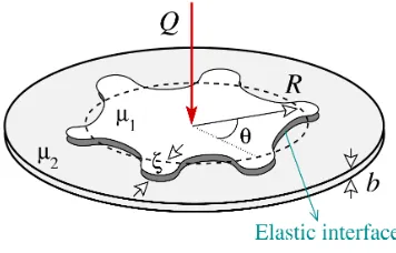
FIG. 1. (Color online) Representative sketch of a radial flow in a circular Hele-Shaw cell with an elastic interface (dark gray boundary) separating the inner fluid 1 and the outer fluid 2 (light gray region).

that in Ref. [24] the production of side-branching pat-terns is not related to the non-Newtonian nature of the fluids, but a result of the interplay between elastic and viscous effects.

In this work we examine the important maximum vis-cosity contrast (A= 1) situation investigated in Ref. [24], and try to assess their main numerical results regard-ing the morphology of the patterns via simple analytical means. This is done through the employment of a per-turbative mode-coupling theory of the elastic fingering problem. We show that already at lowest nonlinear or-der, and by considering the coupling of just three specific Fourier modes, one can reproduce the onset formation of both finger tip-splitting and, most importantly the side-branching phenomena. A morphological diagram is pro-posed for the pattern formation problem, where the pos-sible weakly nonlinear shapes are conveniently described in terms of two controlling dimensionless parameters: the rigidity fractionCand the quantity Γ which expresses the relative strength between elastic and viscous effects. Fi-nally, the occurrence of the possible shapes is discussed in the light of an interfacial bending rigidity field, which is consistent with the weakening curvature effect proposed in Ref. [20] where interfacial elastic fingers arise more easily in regions of lower bending rigidity.

II. PHYSICAL PROBLEM AND GOVERNING

EQUATIONS

Consider a circular Hele-Shaw cell of gap thickness

bcontaining two immiscible, incompressible, Newtonian viscous fluids (see Fig. 1). Fluid 1 is injected into fluid 2 at a constant injection rateQ(equal to the area cov-ered per unit time). Due to a chemical reaction there exists a gel-like interface separating the two fluids. As in Refs. [20–24] we treat the interface as an elastic mem-brane, presenting a curvature-dependent bending rigidity as given by Eq. (2). Notice that in this work we follow Ref. [24] and focus on the maximum viscosity contrast situation in whichµ2≫µ1 such thatA→1 in Eq. (1).

non-3

linear analysis, the perturbed fluid-fluid interface is de-scribed as R(θ, t) = R(t) +ζ(θ, t), where θ represents the azimuthal angle, andR(t) is the time dependent un-perturbed radius R = R(t) = pR2

0+Qt/π, with R0 being the unperturbed radius at t = 0. Here, ζ(θ, t) = P+∞

n=−∞ζn(t) exp (inθ) denotes the net interface

pertur-bation with Fourier amplitudesζn(t), and discrete wave

numbers n. Our perturbative approach keeps terms up to the second-order inζ. In the Fourier expansion ofζwe include then= 0 mode to maintain the area of the per-turbed shape independent of the perturbation ζ. Mass conservation imposes that the zeroth mode is written in terms of the other modes asζ0=−(1/2R)P

n6=0

|ζn(t)|2.

For the quasi-two-dimensional configuration of the Hele-Shaw cell (very small gap thicknessb), the flow is as-sumed to be potential [19–24]. Creeping flow would only result if the plates are farther apart (largeblimit), which is not the case here. So, for our current smallbsituation, the gap-averaged flow velocity isv_j =−∇φ_j, whereφ_j

represents the velocity potential in fluids j = 1,2. The equation of motion of the interface is given by Darcy’s law [1, 2, 20, 21]

A

φ1+φ2 2

−

φ1−φ2 2

=− b

2 ∆p

12(µ1+µ2)

, (3)

where

∆p= (p1−p2)|r=R−(p1−p2)|r=R, (4)

(p1−p2)|r=Rdenotes the pressure jump on the perturbed

interface, and (p1−p2)|r=R represents the pressure jump

on the unperturbed interface. Similarly to what was done in [20, 21] the contributions coming from the elas-tic nature of the fluid-fluid interface are introduced via a generalized Young-Laplace pressure boundary condition, which expresses the pressure jump across the perturbed fluid-fluid interface as

(p1−p2)|r=R=−

1 2ν

′′′_κ2

κ2

s−ν′′

3κκ2

s+ 1 2κ 2 κss

−ν′

1 2κ

4 + 3κ2

s+ 2κκss

−ν 1 2κ 3 +κss

, (5)

where the curvature-dependent bending rigidityν=ν(κ) is given by Eq. (2). In Eq. (5) the primes indicate deriva-tives with respect to the curvatureκ, while the subscripts ofκindicate derivatives with respect to the arc lengths. To obtain a mode-coupling differential equation for the evolution of the perturbation amplitudes, first we de-fine Fourier expansions for the velocity potentials, which obey Laplace’s equation ∇2_φ

j = 0. Then, we express φj in terms of the perturbation amplitudes ζn by

con-sidering the kinematic boundary condition n·∇φ₁ = n·∇φ2, which refers to the continuity of the normal ve-locity across the interface. Substituting these relations,

and the modified pressure jump condition Eq. (5) into Eq. (3), always keeping terms up to second-order in ζ, and Fourier transforming, yields the dimensionless mode-coupling equation (forn6= 0) [8, 21]

˙

ζn= Λ(n)ζn

+ X

m6=0

[F(n, m)ζmζn−m+G(n, m) ˙ζmζn−m], (6)

where the overdot denotes total time derivative,

Λ(n) = 1

R2(A|n| −1)

+ Γ

2R5|n|(n 2

−1)

A1(C, η)(n2+ 1) +A2(C, η),

(7)

is the linear growth rate,

Γ = b

2

ν0π 6(µ1+µ2)Qλ3

(8)

measures the ratio of elastic to viscous forces,

A1(C, η) =Ce−η(−4η 2

+ 10η−2)−2(1−C), (9)

A2(C, η) =Ce−η(8η2−22η+ 5) + 5(1−C), (10)

andη= (1/R)2_{. We point out that Γ = 1/J}ˆ_{, where ˆJ is} a parameter originally defined in Ref. [24].

The second-order mode-coupling terms are given by

F(n, m) = |n|

R ( A R2 1

2 −sgn(nm)

− ΓCe

−η

R5 h

B1(n, m) +ηB2(n, m)

+η2

B3(n, m) + 2η3B4(n, m) i

,

− Γ(1−C)

R5 B1(n, m) )

, (11)

and

G(n, m) = 1

R{A|n|[1−sgn(nm)]−1}, (12)

where the sgn function equals±1 according to the sign of its argument. The expressions for the functionsB1(n, m),

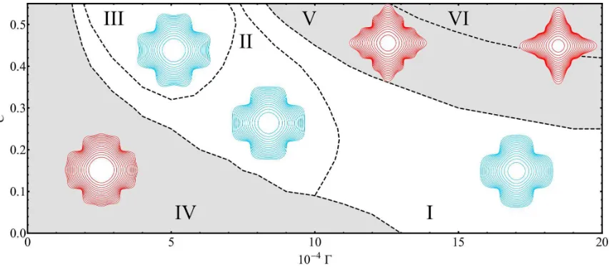
FIG. 2. (Color online) Elastic fingering morphology diagram in the parameter space (Γ,C). The dashed lines delimitate the boundaries separating six different morphological regions (I-VI). Regions I, II, and III are characterized by finger tip-broadening, finger tip-flattening, and finger tip-splitting, respectively. Conversely, regions IV, V, and VI present various manifestations of side-branching events.

III. ACCESS TO FINGER TIP-SPLITTING AND

SIDE-BRANCHING VIA A WEAKLY NONLINEAR FORMULATION

A. Nonlinear fingering dynamics

By following Refs. [8, 30, 32], in order to address the onset of tip-splitting and side-branching events in the elastic fingering problem, we rewrite the net inter-face perturbationζ(θ, t) in terms of three specific cosine modes, namely the fundamental moden, and its first and second harmonic modes 2nand 3n

ζ(θ, t) =ζ0 + an(t) cos(nθ)

+a2n(t) cos(2nθ) + a3n(t) cos(3nθ), (13)

where for a given mode an(t) = ζn(t) +ζ−n(t) denotes

the real-valued cosine amplitude, and

ζ0=− 1

4R(t){[an(t)] 2

+ [a2n(t)]

2

+ [a3n(t)]

2

}. (14)

Without loss of generality, as in Refs. [8, 30, 32] we choose the phase of the fundamental mode so thatan >0.

Within the scope of our second-order mode-coupling theory, finger tip-splitting, finger tip-broadening, and fin-ger tip-narrowing are related to the influence of a funda-mental mode n on the growth of its harmonic 2n. It has been shown in Ref. [8] that an enhanced tendency of the fingers to get wider (narrower) occurs when a2n<0

(a2n > 0). So, a negative growth for the cosine

am-plitude of the first harmonic mode 2n would mean ten-dency toward finger tip-splitting formation. A similar second-order mechanism refers to the side-branching phe-nomenon, and has been proposed in Refs. [30, 32]. In the realm of a mode-coupling model, it has been verified that

side-branching formation requires the presence of mode 3n. If the harmonic mode amplitudea3n is positive and

sufficiently large, it can produce interfacial lobes branch-ing out sidewards which we interpret as side-branchbranch-ing.

It is evident from Eqs. (13) and (14) that to describe the time evolution of the perturbed interface R(θ, t) =

R(t) +ζ(θ, t), one needs to know how the cosine ampli-tudesan(t),a2n(t), anda3n(t) evolve in time. To do that,

we rewrite the mode-coupling equation (6) in terms of co-sine modes, considering the interplay of modesn, 2n, and 3nto obtain

˙

an=λ(n)an+

1

2 {[T(n,−n) +T(n,2n)] ana2n + [T(n,3n) +T(n,−2n)]a2na3n}, (15)

˙

a2n=λ(2n)a2n+

1

2 {T(2n, n)a 2

n

+ [T(2n,−n) +T(2n,3n)]ana3n}, (16)

and

˙

a3n=λ(3n)a3n+

1

2 [T(3n, n) +T(3n,2n)]ana2n, (17)

where

T(n, m) =F(n, m) +λ(m)G(n, m). (18)

For consistent second-order expressions, on the right hand side of Eqs. (15)-(17) we replaced time derivative terms like ˙anbyλ(n)an. The analytical solution for this

type of differential equation has been given in Ref. [8] [see their Eq. (28), plus Eqs. (30)-(32)]. Of course, the time evolution of the amplitudesan(t),a2n(t), anda3n(t)

5

B. Nonlinear pattern morphologies

We begin our discussion by presenting a morphology diagram for the onset of pattern formation in our elastic fingering system. Figure 2 depicts typical representative patterns by considering the parameter space (Γ,C). This diagram reveals that by varying the values of Γ and C

one can identity six basic morphological regions: the first three regions (I, II, III) are related to the occurrence of finger tip-broadening (I), finger tip-flattening (II), and then finger tip-splitting (III). On the other hand, the re-maining regions (IV, V, VI) are associated to the appear-ance of stubby side-branching shapes with pronounced finger broadening (IV), regular side-branching structures (V), and elongated side-branching patterns with stronger finger narrowing behavior. The dashed lines separating the various regions in Fig. 2 are obtained by inspecting the aspect of the resulting patterns while the governing parameters Γ andC are meticulously varied.

Our weakly nonlinear morphology diagram contem-plates the possibility of existence of tip-splitting and closely related events (regions I, II, and III), plus the prevalence of side-branching phenomena (regions IV, V, and VI)), being consistent with the sophisticated nu-merical results reported in Ref. [24]. This can be ver-ified by inspecting the early time stages of the numerical simulations shown in Fig. 5 of Ref. [24], and compar-ing them with the weakly nonlinear patterns shown in Fig. 2. Note that in contrast to what has been done in [24], instead of focusing only on two values of the rigidity fraction C (namely, C = 0 and C = 0.5), we exploited the values ofC for which the elastic fingering instability develops, keeping the linear growth rate pos-itive and bound [20]. In addition, we also have sweeped out the characteristic values of the parameter Γ, within the range 0 < Γ ≤20×10−4 _{(Fig. 5 in [24] only} con-siders Γ = 1/230≈43,4×10−4

). It should be stressed that we have carefully searched for other families of pat-terns within and beyond the range of parametersC and Γ considered in Fig. 2, within an empirically relevant parameter regime, but have not found any other dramat-ically distinct type of patterned morphologies than the ones presented here.

At this point, it should be noted that as in Refs. [33, 34], while plotting the evolving interfaces shown in Fig. 2 and in the remaining figures of this work, we stop the time evolution of the patterns as soon as the base of the fingers starts to move inwards, which would make succes-sive interfaces cross one another. Since this crossing is not observed in experiments [3–7] and simulations [9, 24], we adopt the largest time before crossing as the upper bound time (t=τ) for the validity of our theoretical de-scription. This validity condition can be mathematically expressed as

_dR

dt

t=τ

= [ ˙R(t) + ˙ζ(θ, t)]t=τ = 0. (19)

Notice that, differently from what has been done in

Ref. [34] we evaluate Eq. (19) by taking into account second-order contributions for interface perturbation

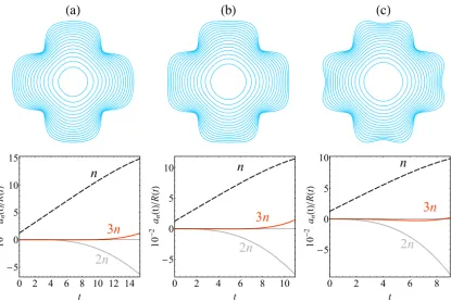
ζ(θ, t), as prescribed by our mode-coupling equation (6). To better appreciate the weakly nonlinear behav-iors expressed by the typical pattern-forming structures shown in regions I, II, and III in Fig. 2, we examine them more closely in Fig. 3. On the top of each panel, we depict the fluid-fluid interface evolution considering the interac-tion of three representative cosine modes (n= 4, 2n= 8, and 3n= 12). On the bottom part of the panels, we plot the corresponding time evolution of the rescaled cosine amplitudes an(t)/R(t) for each of these cosine modes.

This is done for regions: (a) I, (b) II, and (c) III. Similar kind of plots are presented in Fig. 4 for the side-branching regions IV, V, and VI. We stress that all patterns il-lustrated in Figs. 2-5 have the same the initial ampli-tudes att = 0 s an(0) = R0/80, where R0 = 1.5, and

a2n(0) =a3n(0) = 0 so that modes 2nand 3nare both

initially absent. This is done to avoid artificial growth of modes a2n and a3n imposed solely by the initial

condi-tions. This way, the phenomenon of finger tip-splitting and side-branching we study are spontaneously induced by the weakly nonlinear dynamics, and not by artificially imposing large initial amplitudes fora2n anda3n.

More-over, 0 ≤ t ≤ τ, where for each case the final time τ

is obtained from Eq. (19). Even though all the patterns depicted in Figs. 2-5 have the same initial conditions, the innermost interface taken att= 0 may appear to differ in size from plot to plot. This happens because the sizes of some of the shapes have been slightly modified to allow better visualization of their morphological features.

By inspecting Fig. 3(a) for region I (smallCand large Γ), we see a nearly circular initial interface evolving to a four-fingered structure. Note that it is the growth of the fundamental moden= 4 that sets the initial n-fold symmetry for the pattern. Finger tip-widening can be ob-served as time progresses, but the finger tips still present a rounded shape. The broadening of the finger tips is jus-tified by the growth of the negative first harmonic mode 2n (a2n < 0). On the other hand, the pattern shown

in Fig. 3(b) for region II (intermediate values of C and Γ) present fingers that are wider than those shown in Fig. 3(a), and now the finger tips become increasingly flat. This finger tip-flattening behavior is chiefly due to the increased growth of the negative first harmonic mode. Then, by observing Fig. 3(c) for region III (largeC and small Γ) we finally see the occurrence of the finger tip-splitting phenomenon (resulting in typical flowerlike pat-terns) mainly induced by the enhanced growth of mode 2n. It is worth noting that the amplitude of the mode 3n is very small in regions I, II, and III so that side-branching formation is not favored there. However, the small (but non-negligible) growth of the harmonic am-plitude a3n > 0 in regions I and II acts to delay the

FIG. 3. (Color online) Representative elastic fingering patterns of regions I, II, and III (top panel), and the corresponding time evolution of the rescaled cosine amplitudesan(t)/R(t) for modesn= 4, 2n= 8, and 3n= 12 (bottom panel). The values of the

controlling dimensionless parameters utilized in each of the regions are: (a)C= 0.25, Γ = 20×10−4,τ= 15.33; (b)C= 0.35,

Γ = 8×10−4,τ = 10.97; (c)C= 0.55, Γ = 4×10−4,τ= 9.01.

fully nonlinear numerical simulations [2, 9, 24, 28] that the phenomenon of finger tip-splitting is always preceded by the occurrence of finger tip-broadening and flatten-ing. It is also worthwhile to note that if we use the val-ues of the relevant parameters that have been utilized in the numerical simulations of Fig. 5(a) of Ref. [24] (i.e, Γ = 1/230 ≈ 43,4×10−4_{, C = 0, R}

0 = 1, and

an(0) =R0/100) we obtain a weakly nonlinear pattern belonging to region I, consistently with the early time interfacial morphology detected in [24].

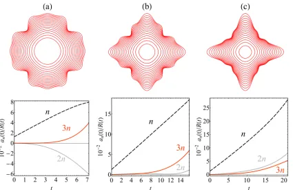
Now we turn our attention to Fig. 4 and focus on the basic morphologies and dynamical responses associated to regions IV, V, and VI. The most evident observation is that the patterned structures depicted in Fig. 4 are quite different from the shapes shown in Fig. 3. For instance, in regions IV, V, and VI there is no sign of finger tip-splitting events. On the contrary, it is clear from Fig. 4 that the most prevalent mechanism is now side-branching. In Fig. 4(a) for region IV (smallC and small Γ) we see the development of an initially fourfold structure which evolves towards a twelve-folded fingered morphology, clearly showing the presence and growth of a sizable mode amplitudea3n>0. Recall that a positive

sign for a3n favors side-branching formation. However,

it can also be noticed that the mode amplitudea2n<0,

a sign that would favor finger widening. As a result of the competition between modes 2nand 3na stubby

side-branched pattern arises in region IV, where the fingers are relatively wide but branch-out sideways. The stubby nature of this particular pattern is partially due to the somewhat restrained growth of the fundamental moden. A different situation is illustrated in Fig. 4(b) for region V (large C and intermediate Γ): now we have the siz-able growth of positive mode amplitudea3n >0 acting

in conjunction with a more moderate growth of a posi-tive mode amplitude a2n > 0 (a sign that would favor

finger narrowing). As a consequence, a more character-istic finger side-branching structure arises in region V. Finally, in Fig. 4(c) for region VI (largeC and large Γ) we still observe a sizablea3n >0, but now accompanied

by a even larger a2n > 0, producing the formation of

side-branching shapes presenting long and narrow finger tips. Once again, if we set the parameters as in Ref. [24] (Γ = 1/230 ≈ 43,4 ×10−4_{, C = 0.5, R}

0 = 1, and

an(0) =R0/100) we obtain a weakly nonlinear pattern belonging to region VI, in line with what is observed at initial times in Fig. 5(b) of [24].

com-7

FIG. 4. (Color online) Representative elastic fingering patterns of regions IV, V, and VI (top panel), and the corresponding time evolution of the rescaled cosine amplitudesan(t)/R(t) for modesn= 4, 2n= 8, and 3n= 12 (bottom panel). The values

of the controlling dimensionless parameters utilized in each of the regions are: (a)C = 0.15, Γ = 1.5×10−4, τ = 7.15; (b) C= 0.55, Γ = 11×10−4,τ = 15.78; (c)C= 0.50, Γ = 15×10−4,τ= 21.02.

plex mode-coupling interactions via a dynamical system expressed by Eqs. (15)-(17), which stability, transitions and bifurcation depend on complicated mode-coupling functions [Eqs. (7)-(12)] on a three-dimensional parame-ter space (C,Γ, A), and thus fairly challenging to ratio-nalize. At this point, we do not have a simple physical ex-planation for this. We hope future analytical, numerical, or experimental studies of elastic fingering in Hele-Shaw cells will further address such an open question.

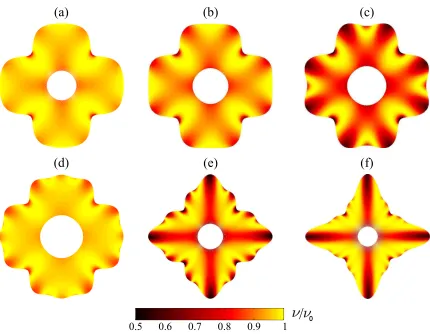
In order to better understand the role of the bending weakening effect of the elastic interface while developing tip-splitting and side-branching morphologies, we depict in Fig. 5 the associated time evolution of the bending rigidity field for the observed patterns in Figs. 3 and 4. The shape-dependence of the bending rigidity entails dy-namical changes expressed by Eq. (2) as the interface evolves in time (0 ≤ t ≤τ). For a given time, we plot how the function ν(t)/ν0 varies along the fluid-fluid in-terface: since the curvature varies along the boundary, the quantity ν(t)/ν0 also changes along the interface. Such changes are expressed by the color coding utilized in Fig. 5: lower values ofν(t)/ν0are represented by dark colors, while larger values of ν(t)/ν0 are associated to lighter colors. The resulting bending rigidity field pat-terns depicted in Fig. 5 are obtained by overlaying the time series ofν(t)/ν0along the associated expanding in-terface at each computed time. Figure 5 shows that

this spatial-temporal dynamics of the bending rigidity for the tip-splitting Fig. 5(a)-Fig. 5(c) and side-branching Fig. 5(d)-Fig. 5(f) phenomena are remarkably distinct. In Figs. 5(a)-5(c) the weakening of the interfacial bend-ing rigidity can be traced back to early stages of the dy-namics, with finger tip-splitting instigated by a sudden increase of the bending rigidity at the tip of the finger. Note however that this increase in bending rigidity does not need be large, and indeed a small increase in the bending stiffness is sufficient to suppress local curvature growth, thus instigating the finger with already reduced rigidity to split.

(a)

(b)

(c)

(d)

(e)

(f)

0.5 0.6 0.7 0.8 0.9 1

/

0

FIG. 5. (Color online) Time evolution of the dimensionless rigidity fieldν/ν0 for the evolving interfaces illustrated in the top

panels of Figs. 3 and 4: (a)-(c) tip-splitting related regions; (d)-(f) side-branching regions.

shear-thinning fluids [25–32]. While for the latter, the viscous resistance decreases with the flow rate, here the interfacial elastic bending resistance is reduced with the local curvature. Incidentally, in Hele-Shaw pattern form-ing structures the regions of large fluid displacement also instigate growth of interfacial curvatures, thus there is phenomenological overlap between these two very dis-tinct systems.

Our current analytical study complements the numer-ical work of Ref. [24] in the sense that the used pertur-bative scheme allows one to explore the whole phase di-agram for morphological changes, whereas the boundary integral method utilized in [24] is quite expensive, and not exactly easy to explore the whole phase diagram. However, it should also be noted that the current work only addresses the initial stages of the instability (at the onset of nonlinearities), while Ref. [24] brings to light the entire dynamic evolution of the system (both initial, intermediate, and fully nonlinear stages of the flow).

IV. CONCLUDING REMARKS

An interesting experimental study on reactive Hele-Shaw flow performed by Podgorskiet al._{[19] has}

demon-strated that visually striking fingering structures arise at the fluid-fluid boundary (e.g., mushroom-shaped and tentaclelike patterns), even if the fluids involved have the same viscosity. This fact motivated He and coworkers [20] to introduce the notion of elastic fingering, in which inter-facial disturbances are not induced by the viscosity dif-ference between the fluids, but are produced by the own elastic nature of a gel-like separating layer. Their weak-ening curvature model treated the two-fluid interface as an elastic membrane presenting a curvature-dependent bending rigidity, and was able to predict the development of interfacial instabilities even in the viscosity-matched case (A= 0). Very recently, Zhao and collaborators [24] revisited the elastic fingering problem, and used sophis-ticated numerical simulations to analyze the pattern for-mation scenario when both elastic and viscous effects act simultaneously. Their elegant numerical results indicated that, under maximum viscosity contrast circumstances (A = 1), one can obtain the emergence of either tip-splitting or side-branching morphologies.

9

the possible physical mechanisms leading to the uprising of finger tip-splitting and side-branching phenomena dur-ing elastic fdur-ingerdur-ing. We have shown that by implement-ing a second-order mode-couplimplement-ing theory, and considerimplement-ing the interplay of just a few Fourier modes (a fundamental moden, and its harmonics 2nand 3n) one is able to cap-ture the most prominent morphological feacap-tures leading to both tip-splitting (enhanced growth of harmonic am-plitudes a2n<0) and side-branching (favored growth of

harmonic amplitudesa3n>0) formation. A weakly

non-linear morphology diagram is provided for the system, being conveniently described by just two controlling di-mensionless quantities: the rigidity fractionC, and a pa-rameter Γ that measures the competition between elastic and viscous effects. Such a morphology diagram is es-pecially useful to provide an understanding of the para-metric conditions required to suppress finger tip-splitting events, and replace them by fingers that side-branch from their tips. Construction of a dimensionless rigidity field for the various possible emerging patterns reinforces the importance weakening curvature effect [20], in the sense that the occurrence of fingering is favored in regions of lower interfacial rigidity.

We are not aware of any existing experimental studies for the elastic fingering problem withA= 1. To the best of our knowledge, the only existing experiments of the problem focused on the viscosity matched case A = 0, and has been presented in Ref. [19]. However, after the publication of the fully nonlinear numerical simulations recently presented in Ref. [24], and of our current ana-lytical weakly nonlinear study, we do hope that exper-imentalists will feel motivated to verify our theoretical, pattern-forming predictions.

In their recent numerical work, Zhao et. al _{[24] have} shown that depending on the parameters and the ini-tial conditions, the patterns can reach a self-similar state or evolve to a limiting shape for which the elasticity of the interface is not important. These effects are illus-trated in Figs. 6 and 7 of Ref. [24]. However, our current second-order weakly nonlinear results do not predict such

stabilization processes.

ACKNOWLEDGMENTS

J.A.M. thanks CNPq for financial support.

Appendix: Functions appearing in the mode-coupling termF(n, m)

This appendix presents the expressions for the func-tionsB1(n, m),B2(n, m),B3(n, m), andB4(n, m) which appear in Eq. (11) of the text

B1(n, m) =−3 + 15

4 m(n−m) + 10(n−m) 2

− 9 2m

2

(n−m)2

−6m(n−m)3

−4(n−m)4

, (A.1)

B2(n, m) = 39

2 −30m(n−m)−71(n−m) 2

+ 81 2 m

2

(n−m)2

+ 54m(n−m)3

+ 32(n−m)4

−12m2

(n−m)4 −12m3

(n−m)3

, (A.2)

B3(n, m) =−14 + 25m(n−m) + 54(n−m)2 −36m2

(n−m)2

−48m(n−m)3 −26(n−m)4

+ 18m2

(n−m)4 + 18m3

(n−m)3

, (A.3)

and

B4(n, m) = 1−2m(n−m)−4(n−m) 2

+ 3m2

(n−m)2

+ 4m(n−m)3 + 2(n−m)4

−2m2

(n−m)4 −2m3

(n−m)3

. (A.4)

[1] P. G. Saffman and G. I. Taylor, Proc. R. Soc. London Ser. A245, 312 (1958).

[2] For review papers, see G. M. Homsy, Annu. Rev. Fluid Mech.19, 271 (1987); K. V. McCloud and J. V. Maher, Phys. Rep.260, 139 (1995); J. Casademunt, Chaos14, 809 (2004).

[3] L. Paterson, J. Fluid Mech.113, 513 (1981).

[4] H. Thom´e, M. Rabaud, V. Hakim, and Y. Couder, Phys. Fluids A1, 224 (1989).

[5] J.-D. Chen, J. Fluid Mech.201, 223 (1989); J. -D. Chen, Exp. Fluids5, 363 (1987).

[6] S. S. S. Cardoso and A. W. Woods, J. Fluid Mech.289, 351 (1995).

[7] O. Praud and H. L. Swinney, Phys. Rev. E 72, 011406 (2005).

[8] J. A. Miranda and M. Widom, Physica D 120, 315 (1998).

[9] S. W. Li, J. S. Lowengrub, and P. H. Leo, J. Comput. Phys.225, 554 (2007).

[10] Y. Nagatsu, Curr. Phys. Chem.5, 52 (2015).

[11] F. Haudin and A. De Wit, Phys. Fluids 27, 113101 (2015).

[12] F. Haudin, J. H. E. Cartwright, and A. De Wit, Proc. Nat. Acad. Sc. U.S. A.111, 17363 (2014).

[14] A. De Wit, K. Eckert, and S. Kalliadasis, Chaos 22, 037101 (2012).

[15] C. Almarcha, P.M.J. Trevelyan, P. Grosfils, and A. De Wit, Phys. Rev. Lett.104, 044501 (2010).

[16] M. Mishra, P.M.J. Trevelyan, C. Almarcha, and A. De Wit, Phys. Rev. Lett.105, 204501 (2010).

[17] L. A. Riolfo, Y. Nagatsu, S. Iwata, R. Maes, P.M.J. Trevelyan, and A. De Wit, Phys. Rev. E85, 015304(R) (2012).

[18] L. A. Riolfo, J. Carballido-Landeira, C. O. Bounds, J. A. Pojman, S. Kalliadasis, and A. De Wit, Chem. Phys. Lett.534, 13 (2012).

[19] T. Podgorski, M. C. Sostarecz, S. Zorman, and A. Bel-monte, Phys. Rev. E76, 016202 (2007).

[20] A. He, J. S. Lowengrub, and A. Belmonte, SIAM J. Appl. Math.72, 842 (2012).

[21] G. D. Carvalho, J. A. Miranda, and H. Gadˆelha, Phys. Rev. E88, 053006 (2013).

[22] G. D. Carvalho, H. Gadˆelha, and J. A. Miranda, Phys. Rev. E89, 053019 (2014).

[23] G. D. Carvalho, H. Gadˆelha, and J. A. Miranda, Phys. Rev. E90, 063009 (2014).

[24] M. Zhao, A. Belmonte, S. Li, and J. S. Lowen-grub, J. Comp. Appl. Math. (to appear), http://dx.doi.org/10.1016/j.cam.2015.11.016.

[25] A. Buka, P. Palffy-Muhoray, and Z. Racz, Phys. Rev. A

36, 3984 (1987).

[26] H. Zhao and J. V. Maher, Phys. Rev. E47, 4278 (1993). [27] L. Kondic, P. Palffy-Muhoray, and M. J. Shelley, Phys.

Rev. E54, R4536 (1996).

[28] L. Kondic, M. J. Shelley, and P. Palffy-Muhoray, Phys. Rev. Lett.80, 1433 (1998).

[29] P. Fast, L. Kondic, M. J. Shelley, and P. Palffy-Muhoray, Phys. Fluids13, 1191 (2001).

[30] M. Constantin, M. Widom, and J. A. Miranda, Phys. Rev. E67, 026313 (2003).

[31] P. Fast and M. J. Shelley, J. Comput. Phys.195, 117 (2004).

[32] J. V. Fontana, S. A. Lira, and J. A. Miranda, Phys. Rev. E87, 013016 (2013).

[33] E. O. Dias and J. A. Miranda, Phys. Rev. E81, 016312 (2010).