MODULATION OF HIGH ENERGY
COSMIC RAYS IN THE
HELIOSPHERE
by
Damian Lindsay Hall, B.Sc., (Hons.)
A thesis submitted in fulfilment of the
requirements for the degree of Doctor of
Philosophy in the University of Tasmania
DECLARATIONS
I certify that this thesis does not incorporate without acknowledgment any material previously submitted for a degree or diploma in any university; and to the best of my knowledge and belief it does not contain any material previously published or written by another person where due reference is not made in the text.
This thesis may be made available for loan and limited copying in accordance with the Copyright Act 1968.
Damian Lindsay Hall
ABSTRACT
The distribution of galactic cosmic ray particles in the heliosphere is influenced (modulated) by the Sun's interplanetary magnetic field (IMF) and the solar wind. The particles diffuse inward, convect outward and have drifts in the motion of their gyro-centres. They are also scattered from their gyro-orbits by irregularities in the IMF. These processes are the components of solar modulation and produce streaming (anisotropies) of particles in the heliosphere. The anisotropies can be investigated at Earth by examining the count rates of cosmic ray detectors. The anisotropic streams appear as diurnal and semi-diurnal variations in the count rates of cosmic ray recorders in solar and sidereal time. Theoretical models of solar modulation predict effects which are dependent on the polarity of the Sun's magnetic dipole (A >0 or A <0). The solar diurnal and North-South anisotropy can be used to test these predictions.
The yearly averaged solar and sidereal diurnal variations in data recorded by seven neutron monitors and ten muon telescopes for the period 1957 to 1990 have been deduced by Fourier analysis methods. The rigidities of the galactic cosmic rays to which these instruments respond encompass the range 10 to 1400 Giga volts (GV). The rigidity spectrum of the solar diurnal anisotropy has been inferred to have a mean spectral index extremely close to zero and an idealised upper limiting rigidity of 100± 25 GV. This is in good agreement with previous determinations. It is shown that this upper limit has a temporal variation between 50 GV and 180 GV and is correlated with the magnitude of the IMF. The rigidity spectrum is likely to be dependent on the polarity of the Sun's magnetic dipole, the spectral index being determined as positive in the A >0 magnetic polarity state and negative in the A <0 polarity state. It is also shown that the amplitude of the anisotropy varies with an 11-year variation and the time of maximum varies with 22-year variation. Both of these variations are shown to be independent of any change in the rigidity spectrum.
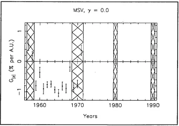
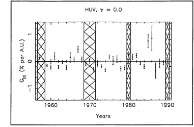
The solar diurnal anisotropy is also used as a tool to calculate the modulation parameters ?Lip, (the product of the parallel mean-free path and radial density gradient) and Gtzl (an indicator of the symmetric latitudinal density gradient). X GII r is found to have a 22-year variation at all rigidities studied and furthermore to only have rigidity dependence when the heliosphere is in the A >0 magnetic polarity state. It is unlikely that XIIGr has any rigidity dependence in the A <0 polarity state. Gizi indicates that below 50 GV the symmetric latitudinal density gradient behaves in accordance with the predictions of current modulation theories. Between 50 and 195 GV however, the predicted behaviour is only observed when the rigidity spectrum of the solar diurnal anisotropy is assumed to be flat, static and have an upper limiting rigidity of 100 GV.
around times of solar minimum. No magnetic polarity dependence of the radial gradient was observed, in direct conflict with conventional theoretical predictions.
ACKNOWLEDGMENTS
In any project of this magnitude there are always many people without whose help the project would have been impossible. It is my hope that I can thoughtfully thank all those who have helped me during the last four years.
In May of 1991 I was fortunate to be sitting in on a postgraduate lecture about cosmic ray physics given by Dr. Marc Duldig from the Australian Antarctic Division and Dr. John Humble from the Physics Department in the University of Tasmania. After the lecture I approached Dr. Humble with the idea of doing my Ph.D. under his supervision. I am indebted to Dr. Humble and Dr. Duldig for giving me the opportunity to work under their joint supervision and for their continual encouragement while undertaking this degree.
For the first half of my tenure I had the pleasure of sharing an office with Dr. Chris Baker. His assistance in introducing me to the Physics Department, Hobart and cosmic ray physics has been invaluable. I thank him for many helpful discussions about modulation theory and his continual barrage of jokes brought back from those mysterious FTP sites.
I would like to express my thanks to the postgraduate students and other personnel in the Physics Department who have helped me during my time there. Special thanks go to Jenny Cramp, Dr. Edward King and Jim Lovell who have always tried to answer any of my queries and I would especially like to thank Judy Whelan for her almost flawless ability to perform any task for me.
I wish to thank the Australian Antarctic Division for allowing me the opportunity to visit Mawson Station for 14 weeks during the southern Summer of 1992-93 to service and modify the cosmic ray telescopes there. I also thank the Australian Antarctic Division, the National Science Foundation of the United Sates and the University of Tasmania for giving me the chance to participate in the joint neutron monitor survey of the Southern Ocean for three weeks during the southern Summer of 1994-95. It was during this time that I was able discuss parts of Chapter 5 with Professor Paul Evenson from the Bartol Institute. I am grateful for his advice towards this thesis, especially his suggestions about treating skew errors and his patient attempts to explain magnetic helicity to me. I thank the Australian Institute of Physics (Tasmanian Branch), the Physics Department of the University of Tasmania, the Astronomical Society of Australia and the Donovan Trust for their financial support in attending interstate and international conferences.
I must also thank Professor Derek S winson for allowing me to use his data from the Embudo and Socorro underground muon telescopes and for sending me the analysed data promptly. Similarly, I wish to extend my gratitude to Dr. Sue Gussenhoven for providing me with polar rain data which allowed me to extend some of the analyses up to the end of 1990. To Dr. Glen McPherson of the Mathematics Department, I thank him for his help in the error treatment in Chapter 3.
Antarctic Division for allowing me to use their word-processing facilities when writing this thesis.
On a personal note I would like to thank my good friends Marc Duldig, Tim Rossiter and Judy Whelan for their moral support over the years. Their assistance has been truly invaluable and will never be forgotten.
Finally, but most importantly I thank my parents Gay and Brian Hall for their devotion to me over the years. They have supported every goal I have ever had and made many sacrifices in order to help me achieve them. They have been an inspiration to me. Without their support this work would have never been possible. Thankyou Mum and Dad.
PREFACE
TABLE OF CONTENTS
DECLARATIONS
iiABSTRACT
ivACKNOWLEDGMENTS
viPREFACE
viiiChapter
1 INTRODUCTION
1
1.1 Preview of the thesis 3
1.2 Review of the literature 3
1.2.1 Theoretical models of solar modulation and their predictions 4
Predictions of modulation models 6
1.2.2 Characteristics of the solar diurnal anisotropy 9 1.2.3 Characteristics of the sidereal (North-South) anisotropy 13 1.2.4 Observations of modulation parameters 15
Radial density gradient 16
Latitudinal density gradient 17
Diffusion coefficients and mean-free paths 19
Summary 20
2 DATA AND METHODS OF ANALYSES
242.1 Cosmic ray observing stations 25
2.2 Atmospheric effects 25
2.2.1 Correcting for the pressure effect 27
2.2.2 Correcting for the temperature effects 27
2.3 Fourier analysis of cosmic ray data 29
2.4 Missing data 32
2.5 Coupling coefficients 34
2.5.1 Nagashima's formalism 35
Using coupling coefficients 39
2.5.2 Calculation of coupling coefficients 40
Coupling coefficients of the Mawson surface and
underground muon telescopes 42
Neutron monitor coupling coefficients at solar maximum and
minimum 43
2.6 Spurious modulations 43
2.6.1 Spurious sidereal diurnal variation 44
2.6.2 Spurious solar diurnal variation 44
Summary 48
3 SOLAR DIURNAL VARIATION
493.1 Theoretical description of the solar diurnal anisotropy 50
3.1.1 The modulation parameter Xip r 55
3.1.2 The modulation parameter Glzi 56
3.2 Data analyses 60
3.2.1 Determining the rigidity spectrum of the sijo - method 1 61 3.2.2 Determining the rigidity spectrum of the U3, - method 2 65
3.3 Rigidity spectrum determinations 68
3.3.1 Method 1 68
Controlling mechanism of Pu 69
3.3.2 Method 2 70
Average rigidity spectrum 70
Magnetic polarity dependent rigidity spectra 72
Yearly averaged SD 74
3.4 The modulation parameters Xipr and Glzi 81
3.4.1 XiiGr 81
3.4.2 Gizt 86
Summary 92
4 SIDEREAL DIURNAL VARIATION-NORTH SOUTH
ANISOTROPY
944.1 Relationship between theory and observations for tNS and
Gr
964.1.1 Theory 96
4.1.2 Relating observations and theory 97
4.2 Data analysis 100
4.3 Results of the North-South anisotropy analyses 105
4.3.1 Rigidity spectrum °f NS 105
Average rigidity spectrum 105
Temporal variations of the rigidity spectrum 106 Solar magnetic polarity dependence 106
Year to year variations. 107
4.3.2 Derived components of I■Is 108
Average 4NS 108
Temporal variation of 4NS 109
Heliospheric polarity variation 109
Year to year variations. 110
The amplitude TiNs 115
The phase ONs 116
4.4 Results of inferring the radial gradient of cosmic rays from tils 122
4.5 Contribution of perpendicular diffusion 125
Summary 126
5 PARALLEL MEAN-FREE PATH
1285.1 Calculating X11 129
5.1.1 Approximate method of calculating X0 129 5.1.2 More accurate method of calculating 2q1 130
5.2 Results 131
5.2.1 Approximate results 131
5.2.2 Effects of perpendicular diffusion 136
The parallel mean-free path, kit 141
Summary 145
REFERENCES
148Appendix
1 SOLAR DIURNAL ANISOTROPY
1562 HARMONIC DIALS IN SOLAR TIME
1583 UPPER LIMITING RIGIDITY TO THE SOLAR DIURNAL
ANISOTROPY
1654 SOLAR DIURNAL ANISOTROPY-BEST FIT RIGIDITY
SPECTRA CONTOUR DIAGRAMS
1725 MODULATION PARAMETERS- XW AND
GIZI 1916 SOLUTIONS TO EQUATION (4.14)
2007 MODULATION PARAMETERS
-N1 2038 DEPENDENCE OF MODULATION PARAMETERS ON
PERPENDICULAR DIFFUSION
2079 PUBLICATIONS
214CHAPTER 1
INTRODUCTION
Galactic cosmic ray particles are high energy nuclei and exist in roughly the same relative galactic abundances as their corresponding atomic elements. Thus most of the galactic cosmic rays are protons. The energies of galactic cosmic rays range from about 10 8 eV to
1021 eV but the accelerating mechanisms of the highest energy galactic cosmic rays are not understood.
The heliosphere is the region of space where the interplanetary magnetic field (IMF) of the Sun dominates the galactic magnetic field. Outside the heliosphere, in the local inter-stellar region the distribution of galactic particles is considered almost isotropic in space and time. Due to random motion and collisions these particles cross the boundary and enter the heliosphere. They will gyrate around the IMF but due to small scale irregularities in the IMF the particles are scattered from their gyro-orbits. The overall motion of the particles will be seen as diffusion from the boundary towards the Sun. Along their diffusive journey the particles will also undergo gradient and curvature drifts in the IMF according to first order orbit theory (Isenberg and Jokipii 1979). The Sun also emits a solar wind plasma radially from its surface with the IMF frozen into it and convects particles back toward the heliospheric boundary. The overall result of these processes is the solar modulation within the heliosphere of the galactic distribution of cosmic ray particles (Forman and Gleeson 1975).
I I
A>0 polarity L4 A<0 polarity I-
11 111 1
A<0 polarity • • • • • - • _ • • • • • •
1960 1970 1980 1990
Years • • • • • „ • • • • , • T •
dilated journey to sea level if their energy is greater than about 2 GeV, and thus be recorded.
At the Earth, primaries streaming in the ecliptic plane are recorded by a cosmic ray telescope
or monitor as a diurnal variation in its counting rate in solar time (Solar Diurnal Variation)
superposed onto a large isotropic component. The streaming of primary cosmic rays
responsible for the solar diurnal variation is known as the Solar Diurnal Anisotropy (4SD)•
The streaming perpendicular to the ecliptic plane is observed as a sidereal diurnal variation in
the count rate of a recording instrument. This streaming is known as the North-South
Anisotropy (4
Ns). Since the anisotropies are produced from solar modulation it is possible
to derive solar parameters such as mean-free paths of particles and gradients in the number
densities from observations of the anisotropies. For example, see the analyses by Yasue
(1980) and Bieber and Chen (1991a).
[image:13.557.87.465.350.626.2]The majority of observations employed for these types of analyses have been obtained from
northern hemisphere detectors, usually neutron monitors. Southern hemisphere observations
and similar analyses at the same and higher primary energies may help to provide new insight
into cosmic ray modulation. By determining the Solar Diurnal and North-South
Anisotropies and deriving modulation parameters, predictions of modulation models can be
tested. Thus, knowledge of the magnetic and solar processes in the heliosphere can be
gained.
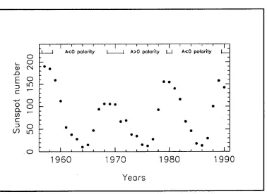
Figure 1.1 Solar activity cycle as represented by the yearly averaged sunspot numbers (Coffey 1993). There is an 11-year cycle for times of minimum sunspot numbers. Solar polarity cycle is determined from the polarity of the Sun's magnetic dipole. A<0 indicates the Sun's northern hemisphere has southern magnetic polarity. A>0 indicates the Sun's northern hemisphere has northern magnetic polarity. The dipole is observed to reverse direction (indicated by the I—I) about every 11 years which implies a 22-year cycle for complete restoration of the dipole direction.
1.1 Preview of the thesis
The following chapters present results of analysing cosmic ray data from neutron monitors and muon telescopes to determine the sidereal and solar diurnal anisotropies of high-energy particles. The rest of this chapter reviews the literature to provide the necessary background information about such anisotropies. Included in this is a review of the basic theoretical models describing modulation and their relation to modulation parameters.
In Chapter 2 the techniques employed in the analyses are presented. Also given is a brief description of the instruments used to collect the data and their locations.
Chapter 3 is concerned with the determination of the solar diurnal variation and the corresponding anisotropy (4s D) of cosmic rays with rigidities in excess of 2 GV. The rigidity spectrum and solar modulation parameters related to the anisotropy are derived. The spectrum is inferred by the use of two novel techniques. Modulation parameters derived from 4SD are presented and compared to theoretical predictions and previous determinations. In Chapter 4 similar techniques to those in Chapter 3 are used to examine the sidereal diurnal variation and the North-South anisotropy at high rigidities. An attempt to derive the rigidity spectrum of the anisotropy is made. From this anisotropy, one of the key modulation parameters - the radial number density gradient (G r) is determined for various rigidities of primary cosmic rays. A comparison is made of the values of these gradients with previous observations and current theoretical predictions. The limitations of this analysis are discussed with special attention paid to the contamination of the results by another anisotropy predicted (Nagashima et al. 1982) but never observed before.
The final chapter concerning data analyses combines the results of Chapters 3 and 4 to derive the mean-free path of cosmic rays of various rigidities up to 200 GV. Some of the mean-free paths are compared to previous determinations while others have never been obtained before. At the end of this chapter the implications of the values of these mean-free paths to solar modulation are discussed, particularly the relative magnitudes of mean-free paths parallel and perpendicular to the IMF.
Finally, the results of Chapters 3 to 5 are summarised and future research problems are discussed. Publications and conference presentations which were produced while undertaking this study are listed in Appendix 9.
1.2 Review of the literature
North-South anisotropy. Finally, the fourth section presents the results of previous determinations of parameters related to solar modulation.
1.2.1 Theoretical models of solar modulation and their predictions
Modulation theories essentially attempt to model the effect of the Sun's interplanetary magnetic field on the distribution of the galactic cosmic rays in the heliosphere. Cosmic rays are influenced by the Sun by three main processes - convection, diffusion and gradient and curvature drifts in the IMF. The IMF is frozen into the solar wind (this is required to keep the Lorentz force on the plasma ions zero) and dragged radially away from the Sun at roughly 400 km sec-1 through the heliosphere. As cosmic rays enter the heliosphere they gyrate around the field lines of force and travel towards the Sun. The IMF is not a completely regular field and contains dynamic irregularities. The gyro-orbits of particles are affected by these irregularities and particles are scattered until a new orbit is found along a regular portion of an IMF line. The net effect of this is parallel and perpendicular scattering of the particles and the motion of the bulk distribution of the cosmic rays can be described by diffusion parallel and perpendicular to the IMF. The same scattering mechanism is partly responsible for the convection of particles outwards from the Sun by the solar wind. Convection is also produced in the cosmic rays' reference frame by an electric field drift (ExB) in the velocity of particles due to the electric field set up in the solar wind plasma and the IMF carried out by the plasma.
The IMF has an Archimedean spiral configuration in the heliosphere caused by the solar wind dragging the Sun's magnetic field radially outward and the solar rotation axis not being aligned with the magnetic axis (for a summary of this process see the review on the IMF by Wilcox 1968 and references therein). The curvature of the field lines and the gradient in field intensity leads to drift velocities of the cosmic ray particles in the interplanetary medium. All these mechanisms combine to produce the solar modulation of galactic cosmic rays. The theoretical basis of modulation was formalised by Forman and Gleeson (1975) and has essentially remained unchanged. The theory presented here is a summary of that formalism plus a brief description of the treatment of the distribution function of cosmic rays from which the theory is derived (Isenberg and Jolcipii 1979; Baker 1993).
If F(x, p, t) is a distribution function of particles such that p2F(x, p, t) d3x dp dS2 is the number of particles in a volume d3x with momentum p to p + dp centred in the solid angle
an
then it can be shown (Isenberg and Jokipii 1979) thatDU
+ V • S = 0
where
qx, p, t)= p2 f F(x, p, t) c1S2 4 n
and S is the streaming vector:
at
(au)
oytK(au
f31 S(x, p, t)= CUV – x(au)1+(eyt)q ar 1+(o.yr)
2
Larx
(1.2)and
co = Gyro-frequency of the particle's orbit; = mean time between scattering;
K = (isotropic) diffusion coefficient;
C = Compton-Getting coefficient (Compton and Getting 1935, Forman 1970); V = solar wind velocity and
U = number density of particles.
The first term of equation (1.2) describes the outward convection of the particles by the solar wind, the second term describes parallel diffusion, the third describes perpendicular diffusion and the fourth involves the gradient and curvature drifts. Writing equation (1.2) in terms of a diffusion tensor
s= CUV – ic • (VU), =
K1 KT 0
-KT K1 0 (1.3)
0 0 x11
where xl, x11, are respectively the perpendicular and parallel diffusion coefficients and the off-diagonal elements are related to gradient and curvature drifts, then
= . (CUV - K VU). (1.4)
Equation (1.4) is a standard time dependent diffusion equation. It is commonly called the transport equation because if we note that
(au)'
)
=v•(E•vu)
at
=
v .(s •vu)+(v • IsA) (vu)
= v •(Ks •vu)+ vD •vu
au
where(
o
— refers to only the non-convective terms in equation (1.4) and x s and icA refer
at
_
to
K being split into symmetric and anti symmetric tensors, we find that V • KA is the driftvelocity (VD) of a charged particle in a magnetic field which has a gradient and curvature. Equation (1.4) is an equation explicitly representing the transport of cosmic rays in the heliosphere by convection, diffusion and drifts as mentioned earlier.
Predictions of modulation models
From 1977 to 1983 a series of papers by Jokipii and co-workers presented the results of numerically solving the transport equation (equation 1.4) for U(x,p,t) including drift processes in the calculations (Jokipii et al. 1977, Isenberg and Jokipii 1978, Jokipii and Kopriva 1979, Jokipii and Thomas 1981, Jokipii and Davila 1981, Kota and Joldpii 1983; hereafter called Papers /, //, III, IV, V and VI). These papers all highlighted the importance of including drifts in the calculations.
Papers I and // showed that because the IMF is characterised by two distinct polarity configurations over 22 years (termed A>0 and A<O, see Figure 1.1) the drifts would have opposite effects on modulation in these two states. Conventional diffusion mechanisms on the other hand, are not dependent on the IMF polarity. The implications of drifts to the transport of poistively charged particles in the heliosphere are that during A>0 IMF polarity states particles will travel into the inner heliosphere from the poles and exit via routes along the heliospheric equator. During A<0 IMF polarity states the particles will predominantly travel into the hefiosphere along the equator and out via high hello-latitudes.
Paper III predicted that these drift effects (coupled to the diffusion of particles) would lead to a larger radial gradient of particles during A<0 epochs than in A>0 epochs. It was also suggested that because of the differences of cosmic ray trajectories during these two IMF configurations (as explained above), the density of particles would be a minimum at the solar equator during A>0 states. Alternatively, during A<0 IMF polarity epochs the drifts of the particles were predicted to produce a local maximum in the density at the equator and a minimum at some higher heliolatitude. This should be observable as a bi-directional (symmetric) latitudinal gradient which reverses direction after every IMF polarity reversal. It was suggested that the inclination of the neutral sheet was an important factor to solar modulation (Kota 1979) and paper IV included this in the numerical calculations. Previously the neutral sheet had only been included as a flat sheet lying on the solar equatorial plane. Results of this model indicated that the neutral sheet was more important to modulation during A<0 epochs than for A>0 epochs. This was explained by the fact that during A<0 epochs particles will travel along the neutral sheet (rather than the solar equator when the neutral sheet is flat). Thus the particles will be affected by the neutral sheet during this IMF configuration more than in the A>0 state when their travelling routes in the heliosphere are from predominantly high latitudes. At high latitudes the neutral sheet is seldom present and is therefore only a small influence on particle transport during A>0 IMF configurations. Paper V was an extension to paper ///. By using a wavy neutral sheet in the calculations and more realistic diffusion coefficients it was shown that the latitude gradient (magnitude and sign) was sensitive to the values of these coefficients. Paper VI was even more realistic (being a full 3-dimensional model) and indicated that the minimum in density at the solar equator during A >0 states predicted by previous models could be displaced by a small distance. Density at the solar equator would never be a minimum, leading to short term observations indicating a negative latitude gradient near the solar equatorial plane for both IMF polarity states. It would seem that considering Figure la of Paper VI (reproduced here as Figure 1.2) a long term average density sample (taken over 10 or so solar rotations) close to the solar equator would yield a minimum in density for this polarity state and hence a
KOTA AND JOKIPII
HEL
IOG
RAPHI
C
Li
—J
90
0
90 180 270 360
HELIOGRAPHIC LONGITUDE
EQUATOR
MIN
■•••■■••
MIN
.7 .8
predicted positive latitude gradient. This gradient is consistent with that predicted by
Jolcipii (1989).
Potgeiter and Moraal (1985) have independently made the same predictions as Jolcipii and
others with a self-consistent model which uses just one set of diffusion coefficients. Their
model predicts a radial gradient of cosmic rays which is smaller during periods of A >0 IMF
polarity and a bi-directional latitudinal gradient which changes direction after IMF polarity
reversals.
Jolcipii and Kota (1989) suggested that the IMF at the heliospheric poles may be less radial
than previously thought. They have incorporated an IMF into their model which has more
transverse field lines at the poles than before. This model predicts an almost invariant radial
gradient at times of solar minimum during different IMF polarity states. This newer model
also predicts that the latitudinal gradient should reverse when the IMF polarity reverses
(Jolcipii 1989). These predictions are supported by the model of Moraal (1990) which
includes a more transverse polar magnetic field.
Baker (1993) numerically modelled the modulation of 1-10 GV particles. The modelling of
10 GV particles is about an order of magnitude larger in rigidity than most researchers
attempt. His results predicted an almost negligible dependence of the radial gradient at
1 A.U. on rigidity.
The theory can be extended to attempt to model the streaming (anisotropies of cosmic rays) caused by solar modulation processes. Some of these models and predictions are presented here as an introduction to the anisotropies which will be examined in the rest of this thesis.
3S By noting that
4 = —
uU
(Gleeson 1969) and defining and in the ecliptic plane with i along the direction of the IMF away from the Sun, it can be shown (Bieber and Chen 1991a) that by transforming the gradient vector into a spherical coordinate system centred on the Sun the components of4
in the coordinate system are4
x
= 4
c
sin x - ki_Gr sin x + pGesgn(B)4), =
sgn(B)pGr sin x + Xi_Go (1.6)4z = 4c cos x - xl
i
G
r
cosx
whereE,c = Compton-Getting anisotropy (3CV/v); x = angle of the IMF with the Earth-Sun line;
=
unit vector in the direction of increasing solar co-latitude; p = gyro-radii of the particles;G
r
=
radial gradient of cosmic ray density; Ge = latitudinal gradient of cosmic ray density;V = solar wind speed;
v = speed of the cosmic ray particles;
anisotropy responsible for the solar diurnal variation;
To define sgn(B) we must realise that the solar wind moving out from the Sun at 400 km sec-1 will cause the two hemispheres of the heliosphere to be separated by a thin magnetically neutral sheet. In one hemisphere the IMF will have a northern polarity and be directed away from the Sun. In the other hemisphere the IMF will have a southern polarity and be directed toward the Sun. The Sun rotates once every 27 days and the neutral sheet corotates with it, passing the Earth at about 400 km sec-1. Since the neutral sheet is wavy and not flat, during a 27 day period the Earth will be alternatively above and below the neutral sheet as the undulations in the sheet overtake the Earth. IMF = A refers to a position in the heliosphere where the IMF is directed away from the Sun. This is called an Away IMF sector. Conversely, IMF = T refers to the opposite side of the neutral sheet - a Towards IMF sector.
Then :
sgn(B) = J+1, IMF = A 1-1, IMF = T
It is through this term in equation (1.6) that drifts affect anisotropies.
Early modellers recognised that by neglecting drift terms in equation (1.6) and other effects such as perpendicular diffusion, vector addition of the remaining streaming components would lead to an overall streaming of particles in a direction parallel to the Earth's orbit around the Sun. The particles would seem to corotate with the Sun. This corotating streaming (or anisotropic flow) of particles could be observed as a diurnal variation in the count rate of a cosmic ray detector as the detector's viewing cone rotated through 360 degrees of space in one day. The anisotropy is the Solar Diurnal Anisotropy. The anisotropy, manifested as a diurnal variation, would have the time of maximum count rate (phase) at 1800 local solar time (streaming along the tangent to the Earth's orbit). This effect has long been known to exist in data from cosmic ray recording instruments (see the next section of this chapter).
Parker (1964) proposed that corotation was a combination of the random walk (scattering by magnetic irregularities) of particles in the IMF and an electric field drift velocity. Forman and Gleeson (1975 and references therein) built on this model and produced the present theory (equation 1.2). They showed that pure corotation will arise if there is no net radial streaming (and drifts are considered negligible). Their model implied that the magnitude of the solar diurnal anisotropy is 0.6% of the average isotropic background flux of cosmic rays. If perpendicular diffusion is not neglected the amplitude of the anisotropy will be less than 0.6% and will be a function of the relative importance of perpendicular and parallel diffusion (see Appendix 1).
Levy (1976) included the curvature and gradient drifts in a model which showed that these drifts could be responsible for changing the direction of the anisotropy in alternate solar cycles. This could explain the 22-year cycle observed in the anisotropy (see the next section). A similar result was obtained by the model of Erdos and Kota (1979). Their model predicted that the direction of streaming during A<0 IMF polarity states should be along the direction of the Earth's orbit. Drifts included in this model were considered responsible for the model indicating that the streaming should change direction during the next IMF polarity state and this streaming would be observed as a diurnal variation with a phase around 1500 in local solar time. This model predicted that the anisotropy's amplitude and phase would be insensitive to rigidity but the amplitude would be sensitive to the neutral sheet warp.
Section 1.2.1 has illustrated some of the predictions of models of solar modulation. The two most important predictions of modulation models which incorporate standard solar magnetic fields are
• Gr
should be smaller during solar minima when the IMF polarity is A >0; and• there should exist a bi-directional latitudinal gradient which reverses direction with polarity reversals of the Sun's magnetic field.
1.2.2
Characteristics of the solar diurnal anisotropy- - -
_
_
^ -
-
_
- -
-
-
_
00 L.T. 12 L.T.
EARTH'S ORBIT 30 km/s
06 L.T.
18 L.T. TO SUN
t
ANISOTROPY=0.5% ECLIPTIC PLANE
Data Insert
-
12 18 2
Local Tine
as cited by Bennett et al. 1932), it was thought that the diurnal variation was related to the
daily variation of some unknown atmospheric effect. Daily variations in cosmic ray intensity
(after the data have been corrected for fluctuations in atmospheric pressure and temperature)
are caused by spatial anisotropies outside the influence of the Earth's atmosphere and
geomagnetic field (see, for example Figure 1.3).
On an individual daily basis the statistical uncertainties associated with the results of the
harmonic analysis are usually quite large. By collecting data over many days and averaging
the results of each day's harmonically analysed data the average solar diurnal variation for
that period is found. Long term averages (from data spans of months or years) are more
precise (the uncertainties being derived from the scatter of the individual days), yielding
information about the average behaviour of cosmic rays in the vicinity of the Earth.
Figure 1.3 Solar diurnal anisotropy in the local time coordinate system. The Earth's rotation causes the asymptotic cone of view of an instrument to sweep through the anisotropy once a day. This gives rise to a diurnal variation in count rate data (insert) with a time of maximum around 1800 local time.
Following the discovery that the solar diurnal variation in cosmic ray data was related to a spatial anisotropy in the primary cosmic ray distribution (Elliott and Dolbear 1951) this anisotropy was, and still is, a greatly studied phenomenon. By the mid 1960's, ionisation chambers had been in operation for over 30 years, collecting data in 2- and 1-hour intervals. Thus began a concentrated effort to understand the solar diurnal variation and the processes responsible for producing the associated anisotropy in galactic cosmic rays.
An asymptotic direction of approach is the direction that a cosmic ray particle is travelling (in free space) before it is deflected by the Earth's magnetic field. Rao et al. (1963) defined the
asymptotic cone of acceptance as "the solid angle containing the asymptotic directions of approach that significantly contribute to the counting rate of a detector." It had been realised that the acceptance cone of a recording instrument depends on its physical dimensions, position on the Earth and the geomagnetic field. The asymptotic cone of a telescope is seldom directly overhead and this causes the recorded phase of the diurnal variation to vary from station to station. By taking account of the asymptotic cones of acceptance of individual instruments, Rao et al. (1963) concluded from two years of neutron monitor data that the solar diurnal anisotropy (4sD) had an invariant amplitude and phase in free space and was caused by an anisotropic streaming of particles coming from somewhere close to 90 degrees East of the Earth-Sun line.
It was assumed that the spectrum of 4SD could be represented as a power law of rigidity
4I --riPT, where ri is an amplitude constant and P is rigidity). It had been realised for some time that there should be some upper limit to the rigidities of particles participating in the solar diurnal variation. The rigidity where the anisotropy vanishes has become known as the Upper Limiting Rigidity (Pu) of 4SD. In reality Pu is the rigidity where the anisotropy ceases to be significant. Rao et al. (1963) showed that the anisotropy was independent of rigidity (y = 0) and Pu was 200 GV.
probably positive while Ahluwalia and Erickson concluded that zero was the best estimate of
While the debate on the correct rigidity spectrum continued the amplitude and phase of the solar diurnal variation were still being investigated in light of the conflicting reports by Rao et al. (1963), Duggal et al. (1967) and Forbush (1967). Duggal et al. (1969) examined the two components suggested by Forbush, concluding that they both had the same rigidity spectrum. Duggal and Pomerantz (1975) conclusively verified there is a 22-year variation in the solar diurnal anisotropy related to the IMF in good agreement with Forbush (1967). They also showed that the variation in the anisotropy of 30 GV particles was larger than in that of 10 GV particles. The variation could not be explained solely in terms of a varying rigidity spectrum. Ahluwalia (1988a,1988b) disputed the existence of the two independent components proposed by Forbush (1967) and Duggal et al. (1969), but conceded that two independent components are present in the anisotropy during the IMF polarity configuration A>0. One of these is aligned with the E-W direction (i.e. at 1800 local solar time) termed the E-W Anisotropy and the other is aligned in the direction radially outward from the Sun, called the Radial Anisotropy. He concluded that the radial anisotropy vanishes during A<0 IMF configurations. The radial anisotropy appearing in alternative sunspot cycles explained the apparent 22-year wave in the phase of the solar diurnal variation. Swinson et al. (1990) analysed about 20 years of underground muon data and correlated the radial component of the solar diurnal variation with the square of the IMF magnitude. This showed that the radial anisotropy was related to the convection of particles away from the Sun by inhomogeneities in the IMF carried out radially from the Sun by the solar wind. The correlation was greater during the A>0 polarity state, interpreted as indicating that the radial anisotropy is more prevalent during this epoch, in agreement with Ahluwalia (1988a,b).
Currently it is believed that the 4SD is a superposition of two anisotropies (E-W and radial anisotropies) at 90 degrees to each other (Ahluwalia 1988a, 1988b; Swinson et al. 1990) contrary to previous conclusions. It is perhaps surprising that Bieber and Chen (1991a) have shown that the solar diurnal variation varies with a period of 22 years around an axis aligned with the IMF; and this axis is very close to the direction of one of the components proposed by Forbush (1967).
The works of Ahluwalia (1988a, 1988b) were consequences of an earlier study. Ahluwalia and Riker (1987) had investigated the solar diurnal anisotropy and its rigidity spectrum from 1965 to 1979, which had continued to be derived inconsistently with previous determinations. Here they concluded that Pu varied in a cyclic manner (in agreement with the above mentioned studies) with low values of Pu at solar minimum and high values of Pu at solar maximum. They showed that the spectral index of the anisotropy's rigidity spectrum could be anywhere between -0.5 and 1.0, with zero or a negative value being the most likely. Alania et al. (1983) had previously analysed data from the world wide network of neutron monitors from 1965 to 1982. They determined the average spectral index for this period to be -0.5, in marked contrast to most studies except for perhaps Jacklyn et al. (1969) and more recently with Ahluwalia and Riker (1987). By 1993, Ahluwalia (1991) and Ahluwalia and Sabbah (1993) had showed that the Pu failed to decrease after solar maximum in 1979 and unexpectedly increased to 180 GV in 1983. This led to a correlation between Pu and the magnitude of the IMF being discovered. The correlation is not only simple but seems intuitively correct, explaining (in part) why relatively large values of Pu and amplitudes of the solar diurnal variation were present during the period 1982-1984. The correlation found by
Nagashima et al. (1987) between the amplitude of the solar diurnal variation (only at rigidities greater than 60 GV!) and the Sun's magnetic dipole moment has also been proposed as partly explaining the large amplitudes in the solar diurnal variation after 1979.
Obviously, much knowledge about the solar diurnal anisotropy has been gained in the past 30 years. The amplitude and phase of the anisotropy are known to have cyclic variations but the exact causes of these variations are not agreed on. The spectral index y and Pu are not completely agreed on although it is generally accepted Pu is always less than 200 GV and declines to values less than 100 GV at times of solar minimum.
1.2.3 Characteristics of the sidereal (North-South) anisotropy
Ionisation chamber data collected for an entire year at half hourly intervals and arranged in sidereal time were examined by Compton and Getting (1935) for an average sidereal diurnal variation. The variation was observed to have a phase at about 2000 local sidereal time. This indicated that the anisotropy producing the variation must have had a fixed direction relative to the stars, unlike the solar diurnal anisotropy which has its direction fixed with respect to the Earth-Sun line. Compton and Getting attributed the sidereal diurnal variation in the data to the motion of our solar system through the galaxy and our own galaxy rotating, producing a relative motion of the Earth through extragalactic cosmic rays towards a declination of 47 degrees and right ascension 20 hours and 40 minutes, sidereal time. Elliot and Dolbear (1951) subsequently found a sidereal diurnal variation in data collected in the southern hemisphere with a phase around 12 hours earlier. Not only did their results indicate that the sidereal diurnal variation was dependent on the hemisphere of observation, but they also indicated that cosmic rays were not produced extragalactically.
Jacklyn (1966) studied the sidereal diurnal variation in underground muon data collected during the 1960s. The two telescopes which were used in the analysis were at the same location (Hobart) but had their asymptotic cones of view directed in the opposite heliospheric hemispheres. The sidereal diurnal variations in the data had a phase around 0600 local sidereal time in the northern heliospheric hemisphere (in good agreement with other observations cited by Jacklyn) and 1800 sidereal time in the southern hemisphere. The discrepancy could not be related to temperature effects and was attributed to a bi-directional streaming of cosmic rays along the galactic magnetic field, prior to entry into the heliosphere. Further discussion of any true galactic anisotropies appearing at these rigidities will be deferred until Chapter 4.
record the excess streaming from the direction corresponding to the flow of particles which
originated in the region of higher density. If the field line reverses direction (the Earth in a
different IMF sector) the excess streaming at Earth will reverse direction. Consequently, at
times, a northern hemisphere telescope will detect a larger intensity of particles than a
southern hemisphere telescope and vice-versa. This is called the North-South Anisotropy
(Ns). The effect was conclusively demonstrated by analysing underground muon data
(Swinson 1971). In reality the streaming of particles perpendicular to the ecliptic plane is a
net anisotropic flow caused mainly by curvature and gradient drifts in the IMF. These results
suggested that the amplitude of
4
NS
was constant during the period 1965-68 and had an
upper limiting rigidity of about 75 GV.
Figure 1.4 The N-S anisotropy in a Towards interplanetary magnetic field (IMF sector. The excess streaming will be from the northern hemisphere (see text).
By 1979,
4NSwas so generally accepted that the IMF sector polarity near the Earth could be
inferred from the anisotropy's observation (Mori and Nagashima 1979). This method of
inferring the IMF sector was shown to be in about 75% agreement with spacecraft
measurements of the sector type.
Yasue (1980) derived the spectrum of
r,Ts for the combined years 1968 to 1972. He found
that the anisotropy was wealdy proportional to the rigidity of the particles (P
0
-
3
) and that Pu
was between 150 and 300 GV. He was the first to show conclusively that the anisotropy was
from the direction perpendicular to the ecliptic plane. He did this by examining all three dimensions of the anisotropy relative to the Earth's equator (i.e. due to the ecliptic plane being tilted 23.5 degrees to the Earth's rotation axis). He examined both of the components of 4NS observable at Earth - a component in the geo-equatorial plane (sidereal diurnal intensity variation) and a component along the Earth's rotation axis (North-South asymmetry in particle intensity). 4NS can be derived from the measurement of either of these variations in intensity. His results were consistent with a time invariant 4Ns.
It is well known that if a solar anisotropy (1 cycle/solar day) is modulated by some seasonal or other process with a period of 1 year (1/365 cycles per solar day) then there will be an apparent variation in the data with 366 cycles a year. This would be present in the data arranged in sidereal time and contaminate a real sidereal diurnal variation. Nagashima et al. (1985) demonstrated that the bi-directional solar anisotropy is seasonally modulated by the yearly variation of the direction of the IMF at the Earth. This leads to a spurious sidereal diurnal variation in cosmic ray data. The appropriate corrections for removing this spurious signal from cosmic ray data were presented, but of course Yasue's analysis (1980) did not incorporate these corrections.
Bieber and Pomerantz (1986) examined the North-South asymmetry component of 4NS from 1961 to 1983 using data from polar based neutron monitors. They concluded that there was a variation in the magnitude of the anisotropy with a ten year period. No dependence of the anisotropy on the solar magnetic polarity was observed.
Swinson (1988) found little variation in the sidereal diurnal variation recorded by underground muon telescopes from 1965 to 1985. He concluded that
4
NS
depends only wealdy on the cycles in solar activity and magnetic polarity.The lack of agreement on the variance (or invariance) of the
4
NS
was increased by an observation which showed that 27-day waves in the amplitude of the 4NS were modulated with a period of 11 years (Swinson and Yasue 1991).Baker et al. (1993a) and Baker (1993) used neutron monitor and muon telescope data to examine the North-South asymmetry from 1982 to 1985. They showed, as expected, that for non-polar instruments the North-South asymmetry was relatively hard to detect, but nonetheless the results indicated that at high rigidities a variation in 4NS does exist.
The 4NS is present in fluxes of particles with rigidities up to at least 150 GV. Although its general characteristics are known, its rigidity spectrum has not been studied in detail. At low rigidities 1,■is seems to have some variation but at P>100 GV it is not obvious from the literature if this variation is definitely present; hence there is much to be learnt from a study of its temporal behaviour.
1.2.4 Observations of modulation parameters
which a scientist can test the predictions of theories by direct and indirect observations of modulation parameters.
Radial density gradient
There are two ways of measuring the radial gradient
(Gr)
of the number density of galactic cosmic rays in interplanetary space. One method is a direct measurement of the gradient by sampling and comparing the density of particles at different spatial positions with spacecraft. The other is by inferringGr
from data collected at Earth by cosmic ray telescopes. Direct observations in space are restricted to measuring particles with relatively low rigidities (less than 5 GV and usually less than 1 GV). On the other hand, gradients inferred from Earth based observations are usually made from monitors which have median rigidities greater than 10 GV and in the case of underground muon telescopes the median rigidity of response is usually greater than 100 GV. Little comparison between the results of the two methods is possible other than a qualitative one. Results presented in this thesis are inferred from Earth based measurements so only a brief review of the results of spacecraft measurements is given here.Most studies of the radial density gradient are made by comparing the spatial difference in density of particles recorded by the Voyager and Pioneer spaceprobes and Earth orbiting satellites such as IMP8. By comparing the counting rates of comparable detectors aboard any two of these spacecraft the magnitude of Gr is usually calculated from the relation :
G = r r2 ln(C/C2) (1.7)
where Ci are the count rates of the instruments and II are the positions of the spacecraft. A time delay for the solar wind propagation from r2 to ri is usually included to ensure that any temporal variability of the radial gradient is removed from the analysis.
Spacecraft observations have consistently reported a positive radial gradient (i.e. greater density of particles further away from the Sun). See, for example the review on radial density gradients by Venkatesan and Badruddin (1990) and references therein. Essentially, most gradients are reported to be about 1 to 4% AU -1 , at various distances from the Earth out to 40 AU. These values of
Gr
are integral measurements, with particles having E >60 MeV/nucleon (rigidity, P >0.4 GV). A key prediction of drift theories (other than those which incorporate a non-standard IMF in the polar regions of the heliosphere) is that the magnitude of Gr is sensitive to the polarity state of the Sun's IMF (see Section 1.2.1). This is not observed, with most studies reporting lower gradients at times of solar minimum than at solar maximum but little or no dependence ofGr
on the solar polarity (Venkatesan and Badruddin 1990, Webber and Lockwood 1991, McDonald et al. 1992).Inferences of
Gr
from data collected by Earth based cosmic ray instruments are made by measuring the North-South anisotropy. (See equation 1.6 and also Chapter 4 for the relation between the North-South Anisotropy andGr).
Swinson (1969, 1971) inferred thatGr
of particles with rigidities greater than 100 GV was positive from 1965 to 1970. This is consistent with spacecraft observations ofGr.
Kudo and Wada (1977) examined the North-South anisotropy of particles with rigidities ranging from 10 GV to 200 GV. They found that
Gr
decreases with rigidity and is lower at solar minimum than at solar maximum. This is consistent with spacecraft observations. Duggal and Pomerantz (1977) inferredGr
from examining the North-South anisotropy derived from 12 years of neutron monitor data (approximately 10 GV particles). They estimated that the averageGr
was about 2% AU-1 at these rigidities from 1964 to 1975. Extending their analysis to the period 1961 to 1983, Bieber and Pomerantz (1986) showed that the averageGr
of 10 GV particles was 1.6% AU-1 andGr
varied periodically, having lower values at solar minima. They found no dependence ofGr
on the polarity of the IMF in agreement with spacecraft observations and verified at higher rigidities (Yasue 1980, Swinson 1988), although Yasue found no significant variation inGr
from 1968 to 1972.Qualitatively, the results from spacecraft observations of
Gr
seem to be consistent with those inferred terrestrially, although the temporal behaviour ofGr
is uncertain.Latitudinal density gradient
In section 1.2.1 it was noted that an important prediction of modulation models which incorporate drift velocities is the existence of a bi-directional latitudinal gradient (symmetric with respect to the neutral sheet). Since about 1970, three techniques have been used to attempt to confirm its existence (or lack thereof). The simplest method (in theory) is that which uses spacecraft separated by some latitudinal distance and compares the counting rates of instruments aboard them. Unfortunately, until recently most space probes have been confined close to the ecliptic plane, with the relatively new data obtained by the Ulysses mission just starting to emerge in the literature. This spaceprobe will eventually pass over both geographic poles of the Sun, making a complete orbit out of the ecliptic plane by around 1998.
Previous reports of latitudinal gradients (Go) from spaceprobes have been conflicting. McKibben et al. (1979) used observations from Pioneer 11 to show there existed a bi-directional latitudinal gradient directed away (positive) from the solar equatorial plane. The data were collected during the A >0 polarity state (1970's) by monitors aboard Pioneer 11 which responded to particles with E >260 MeV. This observation was in good agreement with theoretical predictions. Conversely, negative symmetric latitudinal gradients were reported to exist during the same period (Newkirk et al. 1986), while McKibben (1989) reanalysed the data of McKibben et al. (1979) and concluded that the positive Go present in the heliosphere during 1975-78 was probably uni-directional, contrary to their previous result. During 1981-1990 the LMF polarity was negative (A <0) and theories predict that the bi-directional latitudinal gradient should be directed towards the solar equatorial plane. This has been confirmed (Christon et al. 1986, Cummings et al. 1987, Webber and Lockwood 1992).
The Earth orbits the Sun in a year, during which it ascends to 7.25 degrees north of the solar equator and descends to 7.25 degrees south of the equator. By measuring the intensity of cosmic rays during a year, one can examine any latitudinal variation in the density of cosmic rays across the solar equatorial plane. Any latitudinal variation in density will be observed as a variation in cosmic ray instruments' count rates. Of course, a gradient inferred from any cosmic ray data obtained on the Earth is for primary particles with at least 2 GV of rigidity. A uni-directional Go will manifest as an annual variation while a bi-directional Go will manifest as a semi-annual variation in the data. This method (as reviewed by Venkatesan and Badruddin 1990) has demonstrated that a southward (unidirectional) Go existed during 1960-75. Other studies reviewed by Venkatesan and Badruddin have shown a symmetric Go was present in unison with the uni-directional Go from 1962 to 1973. The symmetric gradient supposedly reversed direction after the solar polarity reversal from 1969-1971. The same technique has also shown that both the uni- and bi-directional Go were present from
1953 to 1979 and both these gradients reversed at solar polarity reversals (Antonucci et al. 1985). Obviously, these results have caused a great amount of uncertainty regarding the form of latitudinal gradients.
The final technique of inferring Go makes use of the gradient and drift velocities of cosmic rays. The direction of streaming due to drifts can be represented as BxG (see equation 1.2). If Go exists, drift fluxes (BxG) in the two hemispheres (separated by the neutral sheet) related to the Go will on average be in the ecliptic plane. This will lead to the solar diurnal anisotropy having an IMF sector polarity dependence. This mechanism was first proposed by Swinson (1970) who showed that during 1967 and 1968 data from an underground muon telescope analysed for the solar diurnal variation indicated a south pointing (uni-directional) Go existed with a magnitude less than Gr. This was verified by Hashim and Bercovitch (1972) by examining the solar diurnal variation in neutron monitor data. The gradient was shown to have a dependence on rigidity of P -0.6 .
Swinson (1976) extended his analysis to encompass the period 1965-73 (which includes the solar polarity reversal during 1969-71). The results indicated that a south pointing (uni-directional) gradient existed across the ecliptic plane for the entire period. The results also indicated that the magnitude of this gradient decreased at times of solar minimum. This conclusion was contradicted by the results of analysing neutron monitor and underground muon telescope data for the solar diurnal variation (Swinson and Kananen 1982). This study indicated that a uni-directional gradient was present during this period which reversed at the solar polarity reversal (1969-1971). Swinson et al. (1986) used four underground muon telescopes to extend this analysis to the epoch 1965-1983. Again the results were interpreted differently from before. The results were interpreted as indicating that prior to 1971, a south pointing uni-directional (asymmetric) gradient existed at the same time as a smaller bi-directional (symmetric) gradient which was directed towards the heliographic equatorial plane. The asymmetric gradient was proposed to be caused by excess solar activity in the northern hemisphere of the Sun. After the IMF polarity reversed they proposed that the asymmetric gradient vanished and the symmetrical gradient reversed direction. Swinson et al. (1991) refuted this explanation and devised a simpler model which assumed that only a symmetric gradient existed, always directed towards the neutral sheet. It was proposed that the neutral sheet can be displaced to heliolatitudes other than the solar equatorial plane due to asymmetric solar activity. This would transform a non-reversing symmetric Go (with respect to the neutral sheet) to an asymmetric Go relative to the Earth. The direction of the apparent unidirectional gradient would be dependent on the hemisphere of the Sun containing excess
activity. This model was not supported by neutron monitor data analysed from 1953 to 1988 (Chen et al. 1991). However, Bieber and Chen (1991a) did conclude that the solar diurnal variation results from analysing neutron monitor and ionisation chamber data supported the view that an IMF polarity dependent symmetric
Go
existed from 1930 to 1988. Chen et al. (1991) showed that the symmetric gradient was present in unison with an asymmetric gradient which had no IMF polarity dependence or observable trends. Ahluwalia (1993) has concluded that the symmetric gradient exists in particles with rigidities up to 300 GV.The existence of a latitudinal variation of cosmic rays is not disputed, however its form (uni-or bi-directional) is. Knowledge of the existence and f(uni-orm of this gradient is a key ingredient to a better understanding of solar modulation.
Diffusion coefficients and mean-free paths
Diffusion coefficients (K) of cosmic rays are related to mean-free paths (X) by
(1.8)
where ij is the speed of the particles (usually taken to be the speed of light).
There are two types of diffusion in the heliosphere - parallel (II) and perpendicular
(1)
to the IMF lines. These are caused by the random walk of particles in the heliosphere. The particles are scattered from their gyro-orbits by irregularities in the IMF and the bulk distribution essentially diffuses along and across field lines (see section 1.2.1 for a more comprehensive explanation). As particle rigidities increase eventually the gyro-orbits are so large that particles will not be effected by the irregularities and regular particle motion will • prevail (Erdos and Kota 1979). Regular motion is just the usual gyration of particles in the IMF combined with the curvature and gradient drifts of their trajectories.The diffusion processes are characterised by parallel and perpendicular diffusion coefficients. These can be related to corresponding parallel and perpendicular mean-free paths, interpreted physically as the average length a particle will travel before being scattered by an irregularity in the IMF and prevented from travelling any further through the heliosphere in that particular direction. For example a small perpendicular mean-free path (X±) implies that the perpendicular velocity of a particle's gyration is often interrupted by irregularities in the IMF. This does not prevent parallel motion continuing and hence parallel diffusion dominates. Conversely, a large Xll would imply that particles seldom have their parallel component of velocity scattered, hence limiting the relative amount of perpendicular diffusion. The theoretical expressions relating to anisotropies incorporate these mean-free paths. By analysing cosmic ray data for the relevant anisotropies, information about the corresponding mean-free path can be obtained.
Not only are the magnitudes of mean-free paths important, but also the relative importance
between 0.001 and 4 GV and that X1 is approximately 0.0067 AU at these rigidities. This would imply that perpendicular diffusion is only 2% to 8.3% as important as diffusion parallel to the IMF. These values of a can be compared to other determinations. Ip et al. (1978) estimated a = 0.26± 0.08 for particles with E>480 MeV (P>0.3 GV). Recently, Ahluwalia and Sabbah (1993) determined that cc must be below 0.09.
By using the solar diurnal variation in neutron monitor and ionisation chamber data, the coupled parameter 2'110r can be determined (see equation 1.6 and Chapter 3). This quantity has been shown to be dependent on rigidity and vary with an 11- and 22-year cycle and is lower at times of solar minima during A>0 IMF polarity states than during A<0 (Bieber and Chen 1991a). It has been shown that this occurs because XII is solar polarity dependent (Bieber and Chen 1991b, Chen and Bieber 1993). These researchers claim that their observations are meaningless in terms of drift theory if a> 0.16, not inconsistent with Ahluwalia and Sabbah's conclusion. On the other hand Ahluwalia and Sabbah (1993) and Ahluwalia (1993) claim that XliGr is rigidity independent. They do find however that Xipr is IMF polarity dependent but make no suggestions as to whether this is caused by a variation in or Gr or both.
Summary
Due to economics and geography most cosmic ray research has been performed from locations in the northern hemisphere. Consequently, many studies of cosmic ray modulation have used data from instruments which have only been directed north of and in the ecliptic plane. The count rates of cosmic ray instruments drop off very quickly as the primary rigidity of response of the instruments increase. This causes the statistical reliability of the data to decrease at higher rigidities so most investigators are loathe to work with instruments like underground muon telescopes. For these reasons analyses of cosmic ray data collected by the University of Tasmania and Australian Antarctic Division can only help to improve our knowledge of the solar modulation of cosmic rays. The data are not only recorded by neutron monitors but an extensive collection of underground muon telescopes responding to primary cosmic rays with rigidities in excess of 150 GV.
The distribution of cosmic rays in the heliosphere is affected by the Sun's interplanetary magnetic field by three different processes. These are convection, diffusion and curvature and gradient drifts. Numerical models suggest that solar modulation of galactic cosmic rays will produce a radial and latitudinal density gradient of the distribution which are both dependent on the polarity of the Sun's IMF configuration. The radial gradient is predicted to always be positive, but smaller during the A >0 polarity state than during the A <0 polarity state. The latitudinal gradient is predicted by the models to be bi-directional and negative (local maximum in density at the neutral sheet) during the A <0 polarity state of the IMF. After a solar magnetic polarity reversal the bi-directional gradient is predicted to reverse direction and have a minimum in the number density at the neutral sheet. It has been noted that newer models now incorporate a solar magnetic field which is less radial at polar heliolatitudes than previously used (Jokipii and Kota 1989, Moraal 1990). These models predict that the radial gradient is not as IMF polarity dependent as previous models. Cosmic
Table 1.1 Predictions and observations of solar modulation parameters
Quantity Model Predictions
Observations P (GV) Notes
Gr IMF polarity Not confirmed. 510 e.g. Potgieter and Moraal (1985) and
dependence others.
No IMF polarity dependence
Confirmed : 1-4% AU-1 1-3% AU-1 3.0±1.1% AU-1
1.8±0.7% AU-1 0.7±0.3% AU-1
0.5±0.2% AU-1 .9% AU-1 .4% AU-1 .3% AU-1 .2% AU-1
510 Jokipii and Kota (1989) and Moraal (1990).
spacecraft Venkatesan and Badruddin (1990). 10 Bieber and Pomerantz (1986) —
10-year variation. 10 Yasue (1980) —
20 negligible temporal variation. 80
150
20 Kudo and Wada (1977) —
80 definite cyclic variation of about 11 150 years.
230
Go Bi-directional 510 e.g. Jokipii (1989) and others. and reverses
direction at IMF
polarity reversal. Confirmed :
spacecraft 10 17 67 130 300 spacecraft 17 00
e.g McKibben et al. (1979) and others. Antonucci et al. (1985).
Bieber and Chen (1991a) — assumed a = 0.01
Swinson et al. (1986). Ahluwalia and Sabbah (1993).
Palmer (1982). Ip et al. (1978).
Chen and Bieber (1993). Ahluwalia (1993). 2% AU-1
0.5% AU-1
0.03% Alrl
Disputed :
All 0.08-0.3 AU
>0.5 AU 0.2 AU 1.0 AU 0.02-0.083 0.26±0.08 50.16 0.09
spacecraft e.g. McKibbin (1989) and others. 130 Swinson et al. (1991).
54 Palmer (1982).
17 Chen and Bieber (1993) — polarity dependent.
10 Yasue (1980).
ray studies can search for the existence of these gradients and estimate their magnitudes. The predictions of these models are summarised in Table 1.1 with the observations which have either supported or refuted their accuracy.
Modulation causes anisotropic streaming of cosmic rays in the heliosphere. The largest non-transient anisotropies are the Solar Diurnal Anisotropy and the North-South Anisotropy. These anisotropies cause a diurnal variation in the count rates of instruments in solar (solar diurnal anisotropy) and sidereal (North-South anisotropy) time. These anisotropies have been the focus of many studies over the years. Although much has been revealed about the anisotropies there still remains some uncertainty about their rigidity spectra and temporal variations.
Many inconsistant derivations of the spectrum of the solar diurnal anisotropy have been reported. The spectral index y has been shown to be anywhere from -0.5 to 1.0. Researchers do agree that Pu is non-invariant and less than 200 GV. It is even agreed that Pu reduces to about 50 GV at times of solar minima and is larger at solar maxima. Just how large however, and the mechanisms responsible for the variation in Pu, is not entirely clear.
Most investigators will agree that the magnitude of the solar diurnal anisotropy is not constant in free-space and has an 11-year cycle. It is also noted that the phase of the anisotropy is rigidity dependent and has a 22-year cycle. One group believe this is due to a contribution to the anisotropy from a component which is directed at 135 degrees east of the Earth-Sun line (Forbush 1967, Duggal et al. 1967, Duggal and Pomerantz 1975; Bieber and Chen 1991a). Another group claim that the responsible agent for this variation is an anisotropy outward from the Sun which is more prominent during the A>0 polarity state (Ahluwalia 1988a, 1988b; Swinson et al. 1990).
Chapter 3 is an analysis concerning the solar diurnal anisotropy. In Chapter 3 the results of analysing cosmic ray data from neutron monitor and underground muon telescopes to obtain the yearly averaged solar diurnal variations are presented. The yearly averaged solar diurnal variations in the data are used to derive the rigidity spectrum of the solar diurnal anisotropy. Two methods for this are explained. The average rigidity spectrum is obtained for the period
1957 to 1990 and the spectra for each year are also derived. These spectra are compared to past determinations, as are the corresponding amplitude and phase of the solar diurnal anisotropy in free space. The temporal behaviour of Pu is examined for correlations with the IMF and other solar quantities in an attempt to explain its variation. It was hoped that this study would dispel some of the contradictions in the literature about the solar diurnal anisotropy.
It has been noted that modulation theories make predictions about radial and latitudinal density gradients. The solar diurnal anisotropy can give information about the latitudinal gradient. This gradient is very controversial due to some investigations inferring a bi-directional gradient which behaves in accordance with theoretical predictions (Antonucci et al.
1985, Swinson et al. 1986, Bieber and Chen 1991a) while others dispute these claims. Included in Chapter 3 is the inference of the latitudinal gradient of cosmic rays with rigidities up to about 200 GV from the solar diurnal anisotropy. The results of this study are compared to theoretical predictions and previous determinations summarised in Table 1.1. Recently, two studies of the solar diurnal anisotropy have investigated the temporal behaviour