High performance Microcontroller Based Transvector Controlled Pulsewidth Modulator Induction Motor Drive

(1)

University of Tasmania

High-Performance

Microcontroller-Based Transvector-Controlled

Pulsewidth Modulator .. Induction Motor Drive

By: Dang Trung Nam Tien

Supervisor: Mr John Arneaud

\!\ o<:.

UY \1\lli

Project submitted in partial fulfilment of the requirements for the degree of

Master of Technology in the Faculty of Engineering, the University of Tasmania,

(2)

Abstract:

(3)

Acknowledgments.

I wish to express sincere thanks to my supervisor, Mr John Arneaund, for his continued support, encouragement, guidance and suggestion through the year.

I am grateful to Mr Gregory The and Mr Quang Ha for their helpful suggestions and technical advice on high performance system design.

I am also grateful to Mr Glenn Meyhew for many helpful suggestion and discussion on digital system design and implementation.

Many thanks go to Mr Bernard Chenary and Mr Steve A very for their valuable assistance in the development of technical aspects of the project.

My thanks also go to all the other members of staff of the Department of the Electrical and Electronics Engineering for their helps through the year.

.l .. v c

\ \

r ' / ,. (

() ( (.\ \ C' ~ ( :{ ~\ 'A t.tt (.(

I ' ' L,

(4)

Table of content

Abstract.

Acknowledgment. ii

1 IM drive system : status and recent trends. 1

1.1 Power inverter. 1

1.1.1 Power semiconductor device. 1

1.1.2 Inverter topology. 2

1.2 Control of Induction Motor. 3

1.2.1 Control technique. 3

1.2.2 Modelling and control design. 3

1.3 Microcontroller. 4

2

Induction Motor and Transvector control. 6

2.1 Induction Motor. 6

2.1.1 Introduction. 6

2.1.2 Steady state characteristics of Induction Motor. 6 2.1.3 Variable-voltage variable-frequency fed Induction Motor. 9

2.2 Transvector control for Induction Motor. 12

2.2.1 Transvector control technique. 12

2.2.2 Coordinate changer. 15

2.2.3 PWM-IM transvector control system. 17

3 Dynamic of PWM-IM drive system.

22

3.1 Introduction. 22

3.2 Mathematic model of system. 23

3.2.1 Model of Induction motor. 23

3.2.2 Model of closed loop system. 24

3.3 Control design. 27

3.3.1 Overview of control design. 27

3.3.2 Torque current loop. 28

3.3.3 Magnetising current loop. 31

3.3.4 Speed loop. 34

3.4 Effects of discrete property on the transient response of system. 42

3.4.1 Sample rate. 42

3.4.2 Effect of quantisation error. 43

4

Variable-voltage variable frequency PWM modulator.

44

4.1 Low frequency PWM. 44

4.1.1 Natural sampling technique. 44

4.1.2 Uniform sapling technique. 47

4.2 High Frequency PWM. 51

4.2.1 Harmonic eliminate technique. 51

4.2.2 PWM operation modes. 53

5

System hardware implementation.

55

5.1 System operation. 55

5 .1.1 Closed loop control system operation. 55

5.1.2 PWM operation. 57

5.2 Control system hardware design. 58

(5)

5.2.2 M68HC11AO microcontroller. 5.2.3 Address latch.

5 .2.4 Data buffer. 5.2.5 Decoder.

5.2.6 EPROM memory. 5.2.7 RAM memory. 5.2.8 High speed oscillator. 5.2.9 16 bit down counter. 5.2.10 Monostable.

5 .2.11 Programmable 8 bit counter. 5 .2.12 Interrupt.

5 .2.13 Interfacing 5-3 Current and speed sensor.

5.3.1 Current sensor. 5.3.2 Speed sensor. 5.4 Power circuitry.

6 System software.

6.1 System software operation. 6.1.1 Selected mode procedure. 6.1.2 Speed procedure.

6.1.3 Current procedure. 6.1.4 PWM procedure.

6.1.5 Load delay time interrupt service routines 6.1.6 Control algorithm.

6.1.7 Processing time.

6.2 Software implementation in C++.

6.2.1 Direct access of peripheral device. 6.2.2 Interrupt programming.

6.2.3 Initialisation for external devices. 6.2.4 Communication programming.

7 Experimental results and evolution.

7.1 Experimental results. 7.2 Evolution and conclusion.

(6)

The IM Drive System- Status and Recent Trends

Chapter 1 : The IM Drive System - Status and Recent Trends.

The technology of solid-state speed control of induction motor (IM) made great strides during the last decades. Traditionally, 1M were considered suitable for constant speed application though complex, inefficient and expensive methods of speed control were known before the advent of the solid-state era. For a long time, de motor were the workhorses in industry for adjustable speed applications.

The induction motor, especially the cage type, seem to possess many distinct virtues in comparison with de machine. These relate to lower cost and weight, lower inertia, high efficiency, improved ruggedness and reliability to operate in a dirty and explosive environment due to the absence of commutators and brushes. Some of these virtues are of paramount importance, which makes the 1M drive mandatory in several areas of application.

In spite of many virtues of IM, the cost of converters and complexity of control requirements are the main factors which are impeding the widespread application of

1M drives in competition with de drives. Therefore, the project intentionally starts with some discussion of the status and recent trends of IM drive system.

1-1, Power inverter :

1-1-1, Power semiconductor device :

The power semiconductor device is the heart of the power inverter. The first invention of the power semiconductor device were the thyristor in the last 1950's. Gradually, other types, such as triac, gate turn - off thyristor (GTO's), bipolar power transistor (BJT's), power MOS field-effect transistor (MOSFET's), insulated gate bipolar transistor (IGBT's), static induction transistor (SIT's) and MOS-controlled thyristor (MCT's) were introduce. In parallel with the new device evolution, the power rating and switching performance of the existing devices began improving dramatically.

+ Thyristor have traditionally been the workhorse in power inverter. Starting originally with the C35 type (800V, 35A) introduced by GE, the modern light-triggered high-power thyristor (6kV, 35kA) have been involving for more than three decades during the thyristor era. The thyristor application is common ranging from several watts to multimegawatt converter.

+ Triac or bidirectional thyristor were invented by GE almost immediately after thyristor commercialisation and found tremendous popularity for medium power inverter. Except for zero voltage ac line switching, the role of the triac will diminish in the future.

+ The GTO, which is another invention of GE that appeared at almost the same time as the triac, was a glimmer of hope, but soon, its research and application were abandoned, considering that device practically has no future. However, from the late 1970's and early 1980's, a number of Japanese corporations introduced high-power GTO's in the market and substantiated that voltage-fed inverters built with self-controlled GTO's have considerable efficiency, size, and reliability advantages over those with force-commutated thyristor. However, the GTO has large switching loss and shows a second breakdown problem at turn-off that demands a large turn-off snubber. The loss consideration also restricts switching frequency typically below one kHz.

(7)

diodes (as high as 1200V, 800AO gradually pushed the voltage-fed transistor inverter rating up to several hundred kilowatts. Higher switching frequency (several kilohertz) and, consequently, the reduced snubber size were definite advantages over the GTO converter. Power MOSFET's also found a large market acceptance, but because it is majority carrier high-frequency high-conduction drop ( especially for high-voltage rating) device, it is dominant in high-frequency low-power applications.

+ The introduction of the IGBT in the early 1980's has brought a visible change in the trend of the power inverter, The IGBT is a hybrid device that combines the advantages of the MOSFET and the BJT. The device is slightly more expensive than BJT's, but the advantages of the higher switching frequency , MOS gate drive, the absence of the second brokendown problem, snubberless operation, reduced the Miller feedback effect, and the availability of the monothilic gate drive with 'smart' capability provides the overall system advantage to the IGBT power inverters.

+ A device that is showing tremendous future promise is the MOS-controlled thyristor (MCT). The MCT is basically aMOS-gated thyristor that can be turned on or off by a small pulse on the MOS gate. The device was announced by GE in November 1988 then was commercially introduced in 1992. Considering that it is new device and there is future evolutionary improvement potential, MCT's are expected to have a significant impact in medium to high power inverter.

1-1-2, Inverter topology.

Converters are generally classified into two types : square wave and pulse width modulated inverter. The square wave inverter was introduced from the beginning of 1970's. It has high efficiency and its simplicity of control has made this class of converter popular in application. However, the disadvantages are that square wave control generates 5th, 7th, 11th ... harmonics that create a rotating magnetic field moving much faster than that of the fundamental frequency and therefore the rotor appears to be stationary to the harmonics. This can be eliminated by using multi-phasing technique, ie more than 6 stepped wave is generated by mixing the phase shifted inverter voltage through a multi-winding transformer or machine. Such a complex and expensive system can be justified only for high power.

The square wave inverters are normally used in low to medium power where the speed ratio is usually limited to 10:1. Recently, this type of drive has largely been superseded by the PWM drive which will be described next.

(8)

The IM Drive System - Status and Recent Trends

1-2, Control of induction motor. 1-2-1, Control technique:

A simple, economic, but low-performance control method of induction motor that is extremely popular in industry is the open-loop V/Hz control technique. A small drift in speed and air-gap flux due to a fluctuation in load torque and supply voltage as well as sluggish transient response, are of no consequence in the majority of application. Scalar speed and position feedback system with inner flux, torque, and current control loops have been used with increased control complexity where improved performance is necessary.

The concept of transvector control, or field oriented control, which was introduced by Siemens Company in the beginning of the 1980's brought on a renaissance in modern high performance control of induction motor driver. This is known as transvector technique because the control implementation is based on vector transformation from rotating to stationary reference frame and vice versa. With transvector control technique, the dynamics of induction motor drives is similar to that of de motor drives, ie, the transient response is optimal and conventional stability limit does not arise. Therefore, the induction motor-transvector control system has found wide acceptance in industry such as paper mills, textile mills, steel rolling mills, machine tool, servo and robotics.

1-2-2, Modelling and control design.

The control and feedback signal processing of 1M drives are extremely complex. This problem arises because the IM dynamics ( d-q model) is described by a high-order non-linear multi-variable state-space equations and the converter-1M drives is essentially a discrete system. At a particular point, the system can be linearised on the basis of the small signal perturbation. Then, the conventional linear feedback analytical method, such as the Nyquist and Bode plot techniques, can be applied. However, the linearization method requires considering to all operation points of speed range because when the operation point changes, the poles, zeros and gain of the linearized system will also change, mandating a new set of control parameters for the system. Traditionally, a fixed control structure with a fixed set of control parameters is defined so that the worst-case system performance is acceptable. With the user-friendly simulation program (such as SIMNON, ACSL, MATLAB, etc.) available today, the IM drive system can be studied with computer simulation avoiding the laborious analytical techniques

(9)

On the other hand, many attempts are being made to enhance the drive performance by intelligent, self-learning, self- organising control using expert system. fuzzy logic, and neural network techniques. The discussion on IM control technique will remain incomplete without some discussion of these techniques.

Expert system (ES) is a branch of artificial intelligence that deals with planting human expertise in certain domain in computer program with the object of replacing the human expert. Symbolic processing languages, such as PROLOG and LISP, find favour in expert programs, but for high-speed real-time control, the C or Assembly language can be used. Expert system is potentially a very important tool in IM drive application. Fault diagnostics both on-line and off-line can be based onES. Automatic design of the converter and total control system is possible using the database of components. Automated simulation study, generation of the static and dynamic model from test data, and system performance test can be performed with the help of ES. Real time performance optimisation control, control reconfiguration, and fault-tolerant control on the basis of on-line diagnostics are also possible with expert system.

Another important tool for IM control system is fuzzy set theory. The theory was introduced by Zadeh in 1965, but only recently, its application has been receiving a lot of attention in Japan. A fuzzy control or estimation algorithm in IM control system embeds the intuition and experience of operator, designer and researcher. It is good in a system where the model is an unknown or ill-defined, complex non-linear multi-dimensional system with a parameter variation problem such as IM or where the sensor signals are not precise. The fuzzy control is adaptive in nature with system parameter variation. The estimation of speed, torque, flux and slip gain tuning can use fuzzy logic, overcoming the parameter variation problem. Unfortunately, there is no systematic analysis and design procedure, and therefore, fuzzy logic-based design may very time-consuming.

The artificial neural network (ANN) is another potentially important tool for IM control system. The term neural network is analogous to the nervous system in the human brain, where a large number of nerve cells are interconnected by input dendrites and axons. The input parallel signals from a layer of cells are processed, and if the output exceeds a threshold, it is propagated to another layer of cells in parallel through the axons. The ANN learning is complex, and various methods, such as back propagation, harmony theory, Bolzman machines, and competitive learning, have been applied. Very recently, several attempts have been made to apply it to PWM-IM control system [13].

It appears that, in the future, the elements of expert system, fuzzy logic and neural network will be combined to gain performance optimisation for IM drive system. 1-3, Microcontroller.

The control system for IM so far are normally implemented using dedicated analog and digital hardware. Recently, however, microprocessor and microcomputer control of IM drives is receiving wide attention because they not only provide simplification of hardware and improvement of reiiability but permit performance optimisation of the drive system which could not be possible by hardware control.

(10)

With a 12-MHz clock frequency, the 8096 can do a 16 bit addition in l!ls and a 16x16 multiply in 6 1-lS. Therefore, this microcontroller is expected to find wide application in IM control system.

Other competitors in the market are Motorola, Zilog, Texas Instrument, and National Semiconductor. Although National Semiconductor originally introduced 32 bit architecture in 1988, the age of the 32 bit microcontroller truly started with the introduction of Motorola's 68020. At the present, the prominent members of the 32 bit family are Intel's 80486, Zilog's Z8000, etc.

The advantages of microcontroller in IM drive system seem obvious.

The superiority of microcomputer control over the conventional hardware based control can be easily recognised for complex drive system. The simplification of hardware saves control electronic cost and improves the system reliability. The digital control has inherently improved noise immunity which is particularly important here because of large power switching transients in the converter. The soft control can easily be altered or improved in the future without changing the hardware. Another important feature is that the structure and parameters of the control system can be altered in real time making the control adaptive to the plant characteristics. The complex computation and division taking capabilities of microcomputer make possible to apply the model optimal and adaptive control theories to optimise the drive system performance. In addition, powerful diagnostics can be written in software. Microcomputer is moving at such a fast rate that the use of efficient high level language with large hardware integration already is possible, and possibly, VLSI implementation is the next goal.

What role can the microcontroller play in IM drive system? Practically, all the control functions can be implemented by microcontroller. The application areas may include gate-firing control of phase-controlled converter, closed loop control, non-linearity compensation, programmable set-point commands, system monitoring and warning, and data acquisition. Microcontroller has been used for optimal PWM wave generation of an inverter. Powerful microcontroller are permitting transvector control and optimal and adaptive control in IM drive system. The cost of an IM drive system can be reduced by using cheap sensors and by reconstructing precise signals with the micro's intelligent. In many cases, sensor can be completely eliminated, or redundant sensor information can be provided by observer computation. System reliability can be enhanced by micro-assisted fault-tolerant control. As the microcontroller's speed and functional integration improve, it will be used in real time or quasi real time for simulation of the IM control system.

The microcontroller will play an increasingly important role in system test and diagnostic. The data from a system under test can be captured and processed to determine efficiency, power factor, etc. Automated test can be performed on a system, and structure and parameters can be identified.

(11)

Induction Motor and Transvector Control

Chapter 2 : Induction motor and transvector control

2-1, Induction motor : 2-1-1, Introduction.

A three phase IM contains a three phase distributed winding that are housed in slots on the stationary part of the motor, usually called stator. The rotating part of the machine, or rotor, also contains either distributed three phase winding or a cage of interconnected copper bars that serve as rotor winding connector. When the rotor contains a distributed winding, the three phases of these windings are connected to three slip rings the motor shaft and the motor is known as a would-rotor machine or slip ring machine. When a cage of copper bars is used, these bars are electrically connected by end ring inside the rotor, no electrical connection can be made to them and the motor is known as a squired-cage motor or, more simply, a cage motor. One set of three phase windings is connected to a three phase voltage supply and this set becomes the primary or excitation (field) windings. With a slip ring motor either stator or rotor windings may act as primary windings, although invariably the stator is used. With a cage motor, only the stator windings can be used as primary windings. The other set of motor windings, known as secondary windings, is not connected to the electrical supply, but is closed on itself. There is no electrical connection between the primary and secondary windings but these are linked magnetically as in a transformer. It is because the secondary e.m.fs and currents are produced by electromagnetic induction that the motor is known as an induction motor.

As with any form of electric motor, the force on the rotating conductor, and hence the motor torque, is proportional to the product of the armature current and the mutual flux in the air gap.

2-1, Steady-state characteristics of Induction motor

When the stator windings of 1M is supplied by a balanced sinusoidal three phase ac voltage source of electric speed ffi_{1 :}

(2.1)

The resulting three phase currents establish a rotating m.m.f wave that result in a flux wave of constant amplitude rotating at a constant speed known as the synchronous speed ffims :

0)1 27tf1

ffi = =

-rns p p (2.2)

(12)

Under the rotating flux, the rotor of the IM will run at speed

co

that is less than the synchronous speed C0₁₁₁₈ • The speed difference

coms - co

is called slip speed and the

ratio of the slip speed to synchronous speed is called the per-unit speed S :

s

=

coms- co

coms

(2.3)

At steady state, an IM may be characterised by a per-phase equivalent circuit referred to stator as shown in fig 2.1.

A B C

Fig 2.1, Per-phase equivalent circuit of IM (referred to stator)

Suppose that fig 2.1 shown the equivalent circuit of phase A in which v Ao is the phase

voltage, we have :

and:

where:

R1 = per-phase resistance of stator winding, ohm.

jXl =per-phase leakage reactance of stator winding, ohm. jXm =per-phase magnetising reactance of the motor, ohm. R2 =per-phase resistance of rotor winding, referred to stator, jX2 = per-phase leakage reactance of stator winding, ohm.

R2 = k;R.2

X

2

=

k;x.

2

k r --E.!_ : rotor-stator re er constant. f

n2

R.2 : actual per-phase rotor resistance.

xa2 : actual per=phase rotor reactance.

(2.4)

ohm.

(2.5) (2.6)

(2.7)

n1, n2 : number of effective turn on the stator and rotor.

(13)

Induction Motor and Trans vector Control

E

!

Fig 2.2, Per-phase Thevenin's equivalent circuit of IM

where:

<P _tA=--tan 1t ₂ - (XI _R

+

xm )

I

and RO is neglected.

(2.8)

(2.9)

(2.10)

(2.11)

From the per-phase Thevenin's equivalent circuit, the following equations can be derived [1, p.207] :

- The speed-torque characteristic equation of IM :

(2.12)

T

=

motor output torque.

-Critical motor speed and torque :

(2.13)

(2.14)

(14)

T= Pm

=~=-3_r;R

2

(J) (J) ms (J) ms S

1-s Pm = output power

=

3I;R2 ( - - )

s

Pg

=

air-gap power = 3I; R2

s

(2.15)

(2.16)

(2.17)

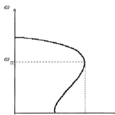
From Eq (2.13), the speed-torque characteristics of an IM can be drawn up when 1M is supplied by a rated voltage/frequency source as in fig 2.3, :

OJ

Fig 2.3, Speed-torque characteristic of an IM at steady-state operation.

2-1-3, Variable voltage-frequency controlled IM:

It was shown in eq(2.12) that the synchronous speed (J)ms of a three phase 1M is proportional to the supply frequency fl. Consequently, the motor speed can be smoothly adjusted from zero up to rated operating speed and higher by increase of the supply frequency fl. However, if the supply frequency f1 is reduced from its rated value while the supply voltage is kept constant, [3, p.236] shows that the motor flux must increase. But operation above the design level would result in excessive core losses and high magnetising current due to an undesirable high level of magnetic saturation. Therefore, in order to maintain operation at the rated flux density when the speed is varied below its rated value, it is necessary to vary the magnitude of supply voltage with variations of its frequency fl.

Controlling IM below rated frequency :

If a is defined as per-unit frequency :

f

a=--~-fl_rated

f1

=

frequency of voltage supply.

f1_ratect

=

rated frequency of motor.

[image:14.591.200.393.249.442.2]

(15)

it will be less than unit (a<l) when frequency of the voltage supply is smaller than rated frequency of motor (f₁< f1_ratect ).

In order to maintain rated motor flux, the e.m.f E must be varied proportionally to frequency fl [3, p.394] :

E

- =

k

=

constant fl

The speed -torque characteristic of IM in this case is derived as following : The reactance of motor can be expressed in general form

Hence: E = aEratect

From the per-phase equivalent circuit of fig 2.1, the rotor current is :

where: as=--""'---a(J)ms- (J)

a(J)ms

The speed-torque characteristic is now obtained from (2.15) and (2.20) :

T = _3_ E~atectR2 I as mms (R₂I as)2

+

x;

R Therefore: s

=

+

-2-m - aX2

T

=+-3_E~ated

111 -2wms

x2

(219)

(2.20)

(2.21)

(2.22)

(2.23)

(2.24)

It can be seen that breakdown the torque Tm is constant because both mms and X2 vary proportionally to frequency fl.

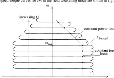
The speed-torque characteristic of IM when frequency f1 is changed and the motor flux is kept constant is shown in fig 2.4.

Controlling IM above the rated frequency :

(16)

The torque expressions for the operation in this range of frequency f1 are obtained by substituting amms for ffims and a(Xt +X₂) for (Xt +X₂) in Eq (2.12) and (2.17) ,

respectively:

(N.m) (a>l) (2.25)

(2.26)

Since a > 1, the breakdown torque Tm decrease with the increase in frequency and speed.

The speed-torque curves for IM in the field weakening mode are shown in fig 2.4 [2].

(J)

increasing

e

"

( -~)

c

~ yonstant power

(

~~

J/ft-mtod

( (J)ms

locus

:c

_~

constant

:c

locus torque

'\. )

·c

~

J:

'

/

[image:16.591.97.464.268.520.2]

-Tm Trated Tm T

Fig 2.4, Speed-torque characteristic for variable frequency control of IM

(17)

2-2, Transvector control

Many different control techniques for controlling an IM has been popular used for a long time [5] : the constant voltage/frequency control, the constant voltage/frequency control with slip regulation, independent torque and air gap flux control (bang bang control, etc. These methods can be classified in to a group called voltage/frequency control that is simple and economical but can be only used for low-performance applications.

In industry application, a high-performance drive system is highly awaited. In this regard, the transvector control technique for the IM is used.

This chapter will analyse the basic control concepts of the transvector technique, then describes its application in PWM-IM drive system.

2-2-1, Transvector control technique.

To analyse transvector control, the operation of IM is considered in the reference frame rotating synchronously with the synchronous electric speed [6] . By such a way, the air gap flux in an 1M can be considered as the flux vector \f' rotating with synchronous speed ffit. Next, the flux vector \f' is considered as an interaction of

-

-stator and rotor voltages and currents Ut, it and h. By this discussion, the balance voltage equations of IM in the reference frame rotating at constant speed ffit are :

where:

-vt

=

Rti1 +p\f't + jcot \f',.

-0= _R2h +p\f'2 + j(cot -ffi)\f'2

-

-\f't = Lti' +Mh

-

-\f'2

=

L2h +Mit

- -*

p is derivative operator.

co

is motor speed.

\f',, \f' 2 are stator and rotor flux.

L 1, L2 are stator and rotor leakage inductances. M is the mutual ( or magnetising) inductance :

M=~L

₂

m

All the rotor quantities are referred to stator.

(2.27)

(2.28)

(2.29)

(2.30)

(2.31)

If a coordinate system with d and q axis is fixed in the rotating reference frame, a

-

(18)

j3

d

Rotating at speecto 1

a Fig 2.6, Decomposed vector N along d and q axis

Decompose equation system (2.27) through (2.32) along d and q axis, gives :

vlct

=

Rlilct +p'I'Ict -mi'I'Iq v lq

=

Rl ilq + P 'I'Iq + ffil 'I'Ict 0

=

R2i2ct + p'¥2ct - ( ffi1 - ffi) 'P2q 0

=

R2i2q + p'¥2q + ( ffil - ffi) 'P2d

(2.32)

(2.33)

(2.34)

(2.35)

and 'P₁ct = L₁_{i1ct + Mi2ct} (2.35)

'P1q = _L1i₁_{q + Mi2}q (2.36)

'P2ct

=

L2i2ct + Milct (2.37)

'P2q

=

L2i2q + Mi₁q (2.38)

The principle of the transvector control lies on the method to control i₁ct and i₁q

currents so that the d-axis coincides with the rotor flux '1'2 as shown in fig 2.7.

j3

d

Rotating at speecto 1

a

Fig 2. 7, Principle of trans vector control : \jf _2d

=

d-axis.

As a result:

(2.40)

(19)

and: - - = 0 d\f'2q dt

From (2.41) and (2.37):

. 1 \TI

=>

12ct

=

- - p r 2

R2

Inserting (2.44) into (2.40), gives :

or

Also, from (2.30) and (2.41):

(2.42)

(2.43)

(2.44)

(2.45)

(2.46)

Equations (2.45) and (2.46) express the fundamentals of the transvector control technique:

*

The rotor flux transients are determined only by the stator current i1ct along the same d-axis, and the transients decay with the rotor time constant T2=L2/R2. Hence, in context of transvector control, i_1ctis called magnetising current.

*

The expression for the torque is similar to that of a separately exited de motor, ie it can be controlled by controlling independently rotor flux \f/₂and current i₁q . Hence, the stator current component i₁q is called the torque current in the present context.

*

If the rotor flux \f/₂ is kept constant, it follows from (2.45) that for p\f/₂= 0,

(2.47)

Equation (2.47) implies that there is no rotor transients and thus the torque current command is instantaneously translated as a torque command. Thus, an ideal response is obtained.

*

The transvector can be expanded into the field weakening mode in which the motor speed is higher than rated the motor speed, the voltage at the inverter input is kept constant and the rotor flux is decreased. It can be seen that for transvector control, decreasing the magnetising current i₁ct , at a constant voltage input, leads to a higher stator frequency co1 . For a constant torque current, per-unit speed S must be constant,

thus higher speeds are obtained : co= co1 (1-S).

Since the torque is given by (2.46), lowering the magnetising current i1ct and keeping

(20)

slower speed response. An increasing in the torque to obtain a higher torque 1s possible by increasing S up to the limit imposed on the total stator current :

I .

1

2

c·

2 . 2)

11

=

3

lid

+

llq

By discussion mentioned above, the control law for rotor flux and magnetising current is drawn up as in fig 2.7

CO rated co _CO_rated co

Fig 2. 7, Control strategy for current i Ict

In the summary, the transvector control technique can be described as following : a) Controlling currents i_1d and i₁q so that the d-axis of the synchronous rotating reference frame coincides with the rotor flux '¥_{2 .}For this, substituting (2.41) into

( 1.45) to obtain control strategy for i_1qand i_{1d :}

(2.48)

b) The IM now can be controlled as de motor, ie by controlling independently the rotor flux '¥₂and the torque current i_1ct.When 1M is controlled below rated frequency

C0_{1_rated ,}the rotor flux '¥₂ is kept constant and equal to its rated value ( E I f

=

const

).In contrast, when IM is controlled above the rated frequency col-rated , the rotor flux '¥₂must be decreased as in fig 2.7.

2-2-2, Coordinate changer:

a, Coordinate changer from static frame to synchronous rotating frame :

In practice, it is necessary to transfer current vector from real time system to static and synchronous rotating system.

Three real time line current ia(t),ib(t),ic(t) are first interpreted into static reference frame by the following formulas :

(2.49)

(21)

Next, the current in static reference a~ frame can be changed into synchronous rotating dq frame:

(2.51)

(2.52)

Equations (2.49) through (2.62) are calculated with help of fig 2.8 [6].

j3

-1. 2c·. ' )

J

-1== - 1

+

1

+

1c .

3 a b d'\ Rotatmg at speedco I

1

!d

a

Fig 2.8, Interpretation between a~ frame and dq frame

b, Coordinate changer from synchronous rotating dq frame to static a~ frame. In many cases, it is necessary to convert a certain parameter from synchronous rotating dq frame to static a~ frame.

Consider the reference voltage expressed in the dq axis in the form of two Vref d yref ,

components Ict an lq •

vref == yref sin(co t

+

8)

1 I 1

and three real time phase voltages are obtained from [6, p.166] :

ref f2cvref 8 yref . 8 )

V AO

=

~

3

ld COS I - lq Slil l (2.54)

(2.55)

vref

=

ficvrefcos(8 -120)- yref sin(8 -120)- -(vref

+

vref) (2.56)

(22)

2~2-3, PWM-IM transvector control drive system :

The PWM and transvector control technique can be combined to produce a high quality PWM-IM drive system.

Concerning flux vector detection, the direct sensing method of the air gap flux by the use of Hall probes is most desirable in theory. From the viewpoint of practical application, this method suffers from high cost and unreliability of the measurement. From this regard, the indirect sensing methods of the rotor flux vector has been developed, which can be divided into two groups. In the first group, the rotor flux vector is obtained by integrating the induced voltage detected directly via sensing coils or calculated indirectly from the stator current and voltage. This method suffers from the inaccuracy of the flux estimation in the low speed region arising from the inaccuracy of the integration. In the second group, the rotor flux vector is estimated from stator currents and rotor speed on the basis of the rotor circuit equations of an IM in the synchronously rotating reference frame with rotor flux vector. Since this method does not require any integration, the rotor flux vector can be estimated even in the standstill. The major weakness of this method is the sensitivity of the estimation to change of rotor parameters, such as rotor resistor, arising from a magnetic saturation and a change of temperature.

On the other hand, in order to realise the high response of current control (to ensure the actual stator current must be adjusted instantaneously and precisely according to their reference current. A fast switching PWM inverter with a local feed back loop is usually utilised for the approximate current control and is sufficient for many industrial applications. However, the high gain current controller is generally required to compensate for the induced voltage. Otherwise, the amplitude and phase error between the actual stator current and its reference become no longer negligible, especially in the high speed region, which deteriorates the vector performance. On the contrary, the high gain current loop produces high acoustic noise, unless the switching frequency of the PWM inverter is extremely high (over 20 kHz). To overcome this problem, another type of current control has been developed in which the stator current are transformed into two de components, that are, a magnetising current component and a torque current component, and then these two de components are controlled, respective to transvector control law.

This section describes a microprocessor based high performance transvector control system in which the indirect rotor flux estimation method and the de current component method are employed.

Fig 2.10, and 2.11, show the configuration of the PWM-IM transvector control system. It can be seen that the system is composed of a current and speed detection, a speed controller, two current controllers, a PMW calculation, a PWM generation, and a transistor inverter. Here, the main parts of system are discussed.

*

Current detection block receives and decomposed three real time line current

current i₁ct (Eq(2.48) to (2.50)). These current components must be controlled independently by the transvector control algorithm.

*

Speed control block gets the reference speed coref from host computer and actual speed co from speed detection. Its output is the reference torque current i~~f .

(23)

order to keep rotor flux o/2 constant. When the motor speed ro increases beyond

co-rated, i~~f must be reduced.

*

Rotor flux position block controls position of the rotor flux '¥₂ to ensure transvector control algorithm : rotor flux must coincide with d-axis of synchronous rotating frame. From (2.48) :

(2.57)

*

Current limiter : in order to protect the transistor PWM inverter from over current, a current limiting function is usually necessary. Here,(in addition to the conventional maximum current limiter in the digital PWM circuit), the current limiting method is also employed, which limits the maximum amplitude of the stator current reference. in fig 2.8, the magnetising current component reference id and the torque current component reference iq are given as the output of the flux and speed controller,

respectively. The explicit expression of the stator current reference is not obtained in this system. Usually the limiters with constant limit value are constituted in order to limit the maximum value of id and iq. However, the disadvantage of these constant

limit value is, for instance, that the magnetising current is suppressed under the constant value, even when the IM is lightly loaded, that is, the value of the iq is small.

This may deteriorates the performance of the transvector control. The amplitude of the stator current reference I1 is expressed as,

The value which should be watched is not id or iq, but I_{1 •} From this reason, the variable current limiting method is employed here. Fig 2.9, shows block diagram of the variable current limiter.

flux controller output

variable limiter

constant

limiter

1_1max

speed controller output

____IL

~

(24)

This limiter enables the system to control i~d in response to i;·q in order to limit the stator current reference so that it does not exceed the preset maximum value I₁_max . It

is of course necessary to put the minimum value in the variable limiter of i;·ct .

*

Two current controller - the magnetising current component controller and torque current component controller- are used to achieve a good performance of system in both steady state and transient operation. Since the quantities to be adjusted by these controllers are de quantities, conventional PI control technique can be successfully employed.

*

Two reference voltage from current controllers are sent to PWM calculation block where time delay and pulse width time PWM signal are determined.

*

Depending on the time delay and pulse width time calculated from the PWM calculation block, the PWM generation block produces PWM signals. Then, PWM signals are amplified and sent to the base gates of power transistor of inverter.

(25)

host computer

RS-232

co

AID

converter

Micro-controller

~ ,lb ,lc.

Fig 2.10, PWM-IM system configuration

~A ~B ~C

Power Rectifier

*

Power Inverter

(26)

-A-B-C

speed calculation

ill

r ~ - - -

-CO+

,~b._

·f,

~

I

J

l11d

cor

1

current calculation voltage calculation PWMI calculation

cor

II 1

Power Rectific

*

~:~

Power

Invert~b

I

~....---,1 ~ PWM PWM

?

t .,...,

CO

rl

~+

·f

I

~

. , ,Vd r Vr

Ks

+

Kstl

J

\~

1 . .

e

r=

taii~q

s

,

+

_'

~

z+~

K,;,l

· ·

_, _,

v'

ct

. - s _r _· _r

COS(!) ₁t , Slll(l) 1 t

generation

I

~ ~

I

' ' &

....

8·

- '

-~--calculation

I

~

(!) l~q

w

_j_

'

-'--I

in~/3(~

- ib /2 -

i

/2~

.

~

i, ib,

t

:t:::t=f-iJ!l=

1/J6 ( ;• -.

U

r

I

;J~~~r ~

I

co;{ferte

:r:=t=t-I1ct= 11a _{COS(!) 1}t

+

1113 SlliD ₁t

, 1. . · r · rt

119= 11p smco 1 t-In cosco 1

~---·---_J~d~~~~oJ

~

(27)

Dynamic ofPMW-IM Drive System

Chapter 3: Dynamics of PWM-IM drive system.

3-1, Introduction :

The dynamics of PWM-IM drive system is extremely complex because of the non-linearity and discrete time nature of the inverter-motor system. For this reason, when a control strategy is developing, it is usually practice to simulate the drive system on the computer and study the performance in detail before proceeding to build a breadboard.

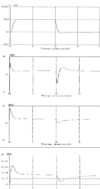
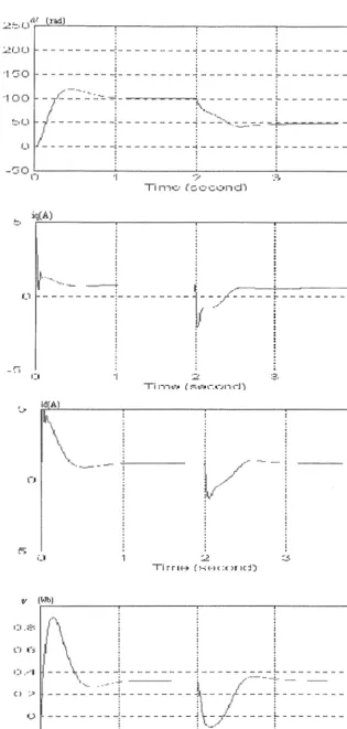
As shown in fig 2.11, the IWM-IM drive system contains three controller : one is to control the reference speed ( speed controller ) and two the others are used to control the magnetising and torque current (current controllers).The problem is what values of the control parameters the system will satisfy the desired dynamic performance. This chapter considers the steps involving the controller design.

There are two main methods to design a digital controller. In the first method, the control design is done as a continuous control system in the s-plane and then simulated in the form of digital system. The second method determines directly the digital controller in the z-plane.

The project employs the first design procedure using frequency response technique to drive satisfactory control parameters. This procedure totally ignores the fact that a sampler and digital computer could influence on the dynamic response and steady state error of real time digital system. Therefore, the last section of this chapter will discuss these effects on implementation of real time discrete system.

Basically, the response of closed loop system to unit step input has the form as shown in fig 4.1.

Here:

point.

Unit response output

-1-'

::::1

CL ...,

::::1

Co

-1-' c <:l

CL 1.4

1.2

1.0

0.8

0.6

0.4

0.2

0.0

t(s)

Fig 3. 1, Unit response specific

tr

=

rise time : time takes the system to reach the vicinity of new set point. ts

=

settle time : time takes the system to decay.

tp

=

peak time : time takes the system to reach the maximum overshoot

(28)

Normally, these requirements are given by customer. In this project, these specifications are supposed as :

+ tr <= 0.2 s + ts <= 0.5 s + 11 <=10%.

3-2, Mathematic model of the PWM-IM drive system.

The first step in control design is to model the overall system. Depending in the actual system, a system can be modelled in the form of mathematical equation, state variable, block diagram , state space or their combination. In this project, the mathematical equation and block diagram method are combined to model the PWM_IM vector control system.

3-2-1, Mathematic model of induction motor IM:

The dynamic properties of an 1M as a control plant can be described by a set of non-linear differential linking stator and rotor currents and voltages with the mechanical quantities (torque, speed and angular position ).

As discussed in chapter 2, an 1M can be described by voltage equations in the synchronous rotating reference dq frame (Eq (2.31) through (2.34)).

Substituting \f_1cl'\f₁q from (2.35) and (2.36) into (2.31) and (2.32), the voltage

equations of an IM in the dq frame can be written in the form of state-space vector [ref 10]:

-rolLa M M

Rl +pLa p

-L2 L2

vld M M 1lct

rolLa Rl +pLa r o

-vlq JL 2 L2 llq

0 _MR2 R _\}'2d

0 _2+p -( rol - ro)

0 L2 L2 _\}'2q

0 M -( rol - ro) R2

L2 L2

(3.1)

In addition, from (2.30) :

T =-P(\f2cti2q - \f2qi2ct) (3.2)

where: P = number of pole pairs.

(3.3)

M =mutual inductance.

(29)

If this condition is held, the system (3 .1) reduces to :

vld Rl +pLa -coiLa vlq

=

coiLa Rl +pLa

0 (3.4)

0 _MR2 ₀

L2

and the generated torque is given as :

(3.5)

From eq (3.4) and (3.5), the block diagram of 1M controlled by transvector technique can be drawn up as fig 3.2 . [10].

3-1-2, Model of the closed loop system:

The block diagram of the feed back control system has been discussed in chapter 2 (fig 2.11). If converter is considered as a proportional block with gain K:

and: K= Jivd

TC

The model of closed loop PWM-IM drive system with transvector control can be shown as in fig 3.3 and fig 3.4. Parameters of proposed motor is shown in appendix A.

v ld

Ol 1

i lq

(30)

(J)

wr · [

llq

TL

(J)l

(31)

Dynamic of PMW-IM Drive System

QProduct

I~ !11t[1jFcn

I

L-EJ

Constant

1 .2*1.25S+ 1.

s

speed control!

l.~H ~GainS

' Pcod"ct1

~I

Gain?

Fig 3.4, System simulation on MATLAB

3.03 0.4S+ 1

Gain1

0.027 0.088s+1 Transfer Fcn5

;r~ 25

~n9 I Sums I 1 .25s+ 1

l...!_J--

Transfer Fen

(32)

Dynamic of the PWM-IM Drive System

3-3, Control design :

It can be seen that the transvector controlled PWM-IM system is described by a high-order non-linear multi-variable state-space equation. Therefore, its control and feedback processing is very complicated. To simplify problem, the conventional design method suggest that the system can be linearized on the basis of the small signal perturbation at a particular operating point and then the conventional feedback analytical methods such as the Nyquist and Bode plot technique can be applied. However, if the operating point changes, the poles, zeros and gain of the linearized system will also change, mandating a new set of control parameters for the system. Therefore, the conventional method requires to check and tune control parameters, theoretically, at all operating point of the speed range, then a fixed control structure with a fixed set of control parameters is determined so that the worse-case system performance is acceptable.

With the availability of user-friendly simulation software packagess such as SIMNON, ACSL, MATLAB, etc, a new method is suggested to avoid such laborious design technique.

It is clear that there is a strong coupling between stator current component and stator voltage component via motion voltage. In order to decouple the motional voltage in the reference voltage, in the proposed method, the motion induced coupling voltages are considered as disturbances to reference voltage. By such a way, two current loops become independent and can be synthesised as linear loops with conventional linear feedback analytical methods.

The synthesis of the speed loop is more complicated due to non-linearity of the system and needs helps of computer. It first is designed by hand, ignores the effects of the rotor flux and then the system is simulated by simulink tool of MATLAB software package to check and tune the parameters of the controllers at all the most important points of the speed region until specified requirements of the system are met.

3-3-1, Overview of control design :

There are many methods that can be used to design a controller such as root locus, frequency response, pole-zero placement, state-space, etc. In this project, the frequency response method is chosen to design the current controllers. The principle of the frequency response method is outlined as follows :

In terms of the frequency response, the transfer function of a system can be expressed by a magnitude I H( (J)) I and a phase I <p( (J)) I curve respect to frequency (J).

These curves are introduced by Bode (1960). By using Bode plot, the stability and dynamic response of system can be entirely analysed through some important factors related to Bode plot diagram. They are :

+ Gain margin GM : is defined as the difference between 1 and I H( (J)) I curve at which the gain of the system is less than the neutral stability value ( phase curve crosses 180°.)

+ Phase margin PM : is the difference between I <p( (J)) I curve and -180° when magnitude curve crosses 1.

The stability and dynamic response of the system now can be stated as :

*

The system is stable when I GM 1>=1 or PM >=0.

(33)

In order to apply the Bode plot diagram technique to design a controller, a dummy function must be introduced depending on the required specifications. If second order could satisfy requirements, the dummy function will has the form :

(3.6)

The formulas related to parameters of the second order dummy function and system specifications are [ 14] :

(3.7)

(3.8)

where:

~

=

damping ratio : (3.9)

ffi₁₁

=

undamped natural frequency (3.10)

After the dummy function is determined, the parameter of the controller is somehow calculated so that its Bode plot of the closed loop system is closed to the Bode plot of the dummy function in the range ( + 15 dB,- 15 dB)

3-3-2, Torque current loop :

In the case of the current loop, the overshoot is permitted up to 25% while the fast response is necessary. Suppose that 11 = 20% and tp = 0.1s are required, the dummy function of torque current loop is derived from (3.6) through (3.10) (appendix B):

30

H c t ( s ) =

-s(0.0167s+ 1) (3.11)

The transfer function of the open loop torque current (without PI controller) is obtained from the torque current block diagram shown in fig 3.3 :

H (s)

=

3.31

ct 0.4s+ 1 (3.12)

I

coupling disturbance

-·*

_{KtcC Ttcs + 1 )} +\

~

3.31

....

s .... + .... _{0.4s +1} ....

-lq

(34)

v~--₀...-. 1 f'L 11'1:::1

PlOO .0 : ;:: :>-<~~~~Jlli~t~~:

:::::;::::;:::

. . . ... , tk~ freq~~y:

.. :

~ ·~ ,_

lllO.Q . ....,.,_··~- _. _{. ..}

.... ... , ...

' . . .

. -·· ·-· ··-. ··-··· ... :·"-...···-····---- ·-·

···-ltl. tJ

: ;::

y~~~~~::::: :~:::1::: i·~>r-~<i:~~

:;: ::;:>;

... , .. , .,.,

··· _ ,

· ·1· · ·

-~ !~~:~-L 11··-~~~~:.

· ·

~

· ·

~

·1

L.or-~~~~:-::~::-::_-::-:~:::~·::-::-:~::~:[~:1-::=::~r~::~-:~}~~~~~~~~~~K~l.-,-::-::-::-::~::~::~:::

(r . - '-:--'---'---L-'----'---'----'---'--'-' -::'-::-.L...L'--'---'--l.:~"'--''-~--'--'-'-'

o.o j::.o 1000.)

:ra.-:=~ ... :;;-)

PhC't:=;.o=-~~ .---PhC't:=;.o=-~~~i·i·"-T~;··i~<:_r·

r

·1

! .... 1 ..

ri

1r ·1

"'

. . . . : -,-~~---L-_J_ o:p~~ loo:p , ,

; ; !

·-·-rT·-·~:

· · ·:,

0:~ ·,+·-~T~y ~=tio+

!

LitJ -so

---1

l?r1

l~U . _~"":--... .

-L80~~--~-~-~~~~--~~~--~~~~~~~~~-~-'-~---~~

::'1r1 ! l . . . . .

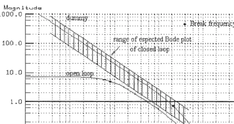
Fig 3.5, Bode plot diagram of the torque current open loop

The Bode plot diagram of the Dummy function Hd and the torque current loop are shown in fig 3.5. Obviously, the dynamic of torque current open loop is much slower than expected (10Hz compares with 60Hz).

When a PI controller is added, the Bode plot diagram of the open loop function will be shifted to the Bode plot of the dummy function. To estimate the parameters of PI control, the gain K1c is first chosen depending on the specification of error due to

decoupling voltage disturbance and is limited by the maximum value :

32

Ktc-max = - ""' 10

3.3 (3.12)

Then, the time constant T₁c is determined so that the Bode plot of the open loop including the controller coincides with the Bode plot of the dummy function. If the gain of the PI controller is chosen equal to the maximum value Ktc-max

=

10, time

constant will be Ttc

=

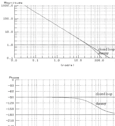
0.4s.

Fig 3.6 shows the Bode plot diagram of the torque current loop with the PI controller and fig 3.7 shows the closed loop unit response. The unit response quite satisfies the specifications, ie it reaches the peak value at tp = O.ls without overshoot. This is explained by the fact that the PI controller completely compensate for the time constant of torque current open loop and therefore the closed loop behaves like a first order system.

(35)

~ra.:j,.. o:

F'h"'""'

~ - · : · · · · : " " : ' : " " ' ' " " ' ' ·:·:" ·: " " " : . . 0 • I • ' ' ~ . • • • .. ' . . a I • ' • • ' • • I . • •

. . . . . . . .

. . . . . . . . :: : : : :

:])

. . . . . . . . .

- 6 ) -·~····~····~·!··· ... -.:·=·· -.: ... ···! :.: ... .: ... .: .. : ... : .. .:.

. . . . : : : : : .l<.> ;~ ~ l<.>q..

1?"1

~...:-... :

0 ' 0 0 ; : : ~N~~N·~~ : : : : :

. . . .

: .

>~. :.'.um.··l)y fiin~~·~

-!5.) _ , , .... , .... ,., ... ,., .. ·: ... : :.: .. . : . .. : .. :.>.•-, ... : .. : . . .

~ ~ : : : : ~ ~ ~ ~ ~ ~ ~ -~~~--j_ ..

: : : :

: : : : : : : :

- 2 0 _ , , .... , .... ,., ... ,., .. ·: ... : :.: .. . : . .. , .. , ... , ..

i 1

I i I

I I i I

i

I

I i

-27) ---L~--~---~--~--~~~--~~--~~~-W

J.: 0.1 L.O ~0 0 ~OC.C 1COC.C.

Fig 3.6, Bode plot diagram of the closed loop torque current

1.5 r - - - . . - - - . , . - - - , . - - - ,

'

' ' '

. --- -:---J-~.,-~~_:-~----

:···-···--··-·-·-·-··----.

.,..,"'" ...

~ /

1

,,./···

,•' I

/

:

0.5 --- .. "---:--- ·- -

---/ '

/

:

/

:

0

---~---~---L---0 '

' ' '

-0.5 L . . . I ___. , L _ _ _ ___,l, _ _ _ ___,_ _ _ _ _ _ _ ,

0

0.05 0.1 0. 5

0.2

Time (second)

(36)

3-3-3, Magnetising current loop:

As discussion shown above, the proposed method to synthesise PWM-IM vector control system suggests that the motion induced coupling voltages can be considered as the disturbance to reference voltage. Therefore, the both the torque and magnetising current loops are decoupled and can be designed as a linear systems.

Fig 3.8 shows the block diagram of the magnetising current loop.

coupling disturbance

-·*

~

KmJ Tmc" +1) +\ + 3.31 ld

+ -j;; _-- I__.

- s 0.4s + 1

ld

-0.027 0.93s ¢

-0.089s+l ~

Fig 3.8, Block diagram of the magnetising current

The transfer function of the magnetising current open loop is derived from fig 3.3 ( see also appendix B ) :

Hmc(s)= 3.31(0.089s+1)

(0.4s+ 1)(0.0885s+ 1) (3.13)

Suppose that the specifications of magnetising current loop are similar to that of the torque current loop, ie 11 = 20% and tp = 0.1s, the dummy function is determined as eq

(3 .11)

Fig 3.9 shows the Bode plot diagram of the dummy function and the magnetising current open loop.

Using the Bode plot technique , the gain of the PI controller is found Kmc = 10 and time constant Tmc = 0.4s

Fig 3.10 shows the Bode plot diagram of the torque current loop with the PI controller and fig 3.11 shown unit response closed loop. The unit response quite satisfies the specifics, ie it reaches the maximum value at tp = O.ls without overshoot. This is explained that the PI controller completely compensate for the time constant of torque current open loop and therefore the closed loop acts as first order system.

By adding the PI controller, the torque current open loop also improves the

steady-state accuracy of the system and reduces the sensitivity to motion induced coupling

(37)

1.0~:-:~:-::-::~::~:;-::~::-~;:-::-::~::-::-:~~:-:~:~~:~i:-::-:~~:-::-:~~:~:i~:~~:~, -.:-:~~:~::~---~::~:;-::~::~;:-::-::~::-::-::~::~:~

:;::::: :):::: ;:::

:;:::::)s:.-·~<L:::)::::

;::

0- 1 LO 10.0 100.0 1000.0

(rad/s)

Phase

0 r---:--'"':""""~-';--'--' :_:_· ·..:__· ·:-::·_:__· : .. : , ..

;~; ;

..

; ; ; ; ; ; ; ; ;

·~·:··,:· ... :·· ., ··-··.' .... , .. ,., ... , .... , .... '

..

::

':

-30

-GO _{·: ·: ·· · ·- · ·· · ·: ·; ·:- · · ·:· · · ·:·-: · 1 ·}_{ofie~·10·~r·:}

_·:·:

. .

-9 0 r--~-~-~-~--~~~""'-'-'-'-'' -~:_:.~-~~~~: .... ~.-..

=~::

· · ·:

1::

t:

j

::::::1::::1 ·:: · 1.: · ·:: 1::::1::::1

t:::

r~~~t-~id~~:

1::::1.:

::

: : : : : : :: .. : :

:::~~~j

-180 ~----~--~~~---~~--~----~----~--~~----~--~~

-ZlO o o • o .. o o I" o , o 1 o o o • .. . ~ o o • .. o • 1 o .. ' I ' 0 0 ' 'I . 0 0 0 0 . . 0 0 I ' .. ' I • 0 ' 0 .. 0 0 0 0 .. ' • I ' . . ' I ' 0 0 • .. 0 ' ' '

. .

. . . .

-240 ... ·-··-·-_.. ... -. _.-···-. _.. . ···-... ·-···.- ... . _.. _.. ·-··-···-· . _.. .. ·-. . _.-··-... --···· . . _.

. . . .

[image:37.591.67.465.225.637.2]

0- 1 1.0 10 . 0 100.0 1000.0

(38)

1000.0

100.0

10.0

::;:::-><. __

:;::::::;::::;::::j::::::j::::;::::

• • 'I • • • • .. • • r :U.,'I. • 1 • • o o ~ ~ • • , 'I , o I , 'I • 1 • • • • ., • , o • 'I • • 1 •

: : : :--"-- : ' ' ' ' :

. . . . . ... . .

' ' : ' • • '~' • ~ '~ • : "'-,,~~:'' • ' I ' ' I • ' I ' I " ' ' : • " ' ' I ' ' I •

:: j::::;::;:

j :::::: j

::">i~~-:

j

:j:::: j::::

j::::

' 'j''' ': '': ': ·: ''''

~-''

':' ':

--->~<' '~''

'' :'': .

: : ; ; ; ; ; ; ' ; ; ; ;;: : : ; : ) ; ; : : ; ; ; : ; ; : : :

:~'·t<~~;

; : ;

. -~ ... -~-·~·~·: ····~~ ... ~. ·:·~·:··· -~"'' ~~~-' ~~~-' ~ ' ' ' ' ~ • ' r ' ~ ' I • • • • ~ a ' ' ' , • • I • • ' I ' • • • , • • • ' , • • I •

' . . . . . ' . . . ... _... . ... _{. . .}. ...

. ..

_... . . ., _.... _{. . .}, . .,., ... ., .. , . .,., .. . ' . . .. ' ' ' .

• • • • • • a t • ' 1 ' 1 ' ' ' . . . , ' ' ' ' I • •

[image:38.591.68.461.78.508.2]

. · · · : · ·:· :·:··. · : · · · · : .. . ... ":. · : · ··:·· .. " : ' ' ' ' " : ' '

... , . .,., .... ., ... . . ... -. ... . . . . . . . . . . -: . -: . ~ . : .... ": .... ": ..

. ... -··-···--.... -.. .... ., .. , . .,., .... ., .... ., ..

. ... . . . . -

..

., ... -., . .... ~ . ..

' ' .

1.0 ~~---~~~--~---~~~--~-~~~~~~~~~~--~--~~~

::::::::::::::::::::::::::::::::::: :; :::::::::::::::: :

::~~d6~~ai6ci~:

. . . .. .. i.-;·~-~ . y .. ~ ..

Phase Q

-30

-GO

0. 1 LO i 0 '0 100.0 1000.0

Crod/s)

, , . , •• ' " ' ' r ' " ' • • • • 'I • . • • • 'I • • I • .. • I • • • • 'I • . • • • 'I • • I • .. • I u ' ' ' 'I • . • • • .. • ~ I ' .. • I • • • • . 'I ' ' ' ' 'I • • I • 'I 'o

. . . .

. . . . . . . .

I I I I I I I I I I I I I I I I I I I I I I I I

, , . , , , . , . . , r , , , ' ' ' ' , . , ' ' ' I ' _. ' 1 ' ' 1 ' 1 ' ' ' ' " ' ' ' ' . . . ' I , , , , . , , , , , ' ' ' " ' • I • . _. , , , , , ' " ' I ' ' ' ' . 'I ' ' I ' " ' I

. . . .

. _.. . _. . _.

o m . o o o • ~ . o o . . n o a o .... -... -.... -... -.... -.... -.. -... -.... ~ . -.. -... --.... -.... -..

: : : · · : : j ~lp~ed lpop j j j j

-go

r-~--~~~--~---~~~----~~~~~~---~~~--~--~~~

=:::

i

!ill

!:T

itT!TIFb~--180

' ~ • • • • ~ ' ' r 0 '1 ° I • • • • 'I • 0 ' ' 'I ' ' I ' .. ' I ' ' ' ' 'I 0 ' 0 ' 'I ' ' I ' • ' I • ' 0 ' 'I ' ' 0 ' 'I ' • I ' 't ' I ' ' ' • .. ' ' ' '

. . . .

-Z10 _. _. _. _. _.

. . . . .

-240 ... _.. . ·-· . _.. ·-·-... ·-· _.. . .... . ···-··· . ... . _.. -· .. . _. ·-··-· ··-· . . _. ···-·-··- ···-- ... . . _. . . _.

. . . .

-270 ~~---L-L~---L--~~~--~--~~~--~~~~~--~~~~

0.0 0 - 1 1.0 i 0 . 0 100.0 1000.0

Fig 3.1 0, Bode diagram of magnetising current-closed loop

1.5.---.---.---.---.

1 - - - -:- - - -~ - - - :::: .... ~ ... :: ... :::-... :::-.... ::: .. .:::::-···""'"'"""'"'"' ,,, .. , .. ..-••""...---~ :

~~---~·· : :

/ , .. ~·: : :