Reducing uncertainty in subdivision optimization

Journal of Shipping and Ocean Engineering 2 (2012) 18-27

Reducing Uncertainty in Subdivision Optimization

Romanas Puisa, Nikolaos Tsakalakis and Dracos Vassalos

Ship Stability Research Centre, University of Strathclyde, Glasgow G20 0TL, UK

Abstract: Design of watertight subdivision inherently involves its optimization with the objective to increase the index “A” above its minimum required value. In view of a big popularity of probabilistic search methods such as genetic algorithms, this task is intrinsically time consuming. Thus, even when an optimal subdivision layout (i.e. topology) is determined, it can be found that the optimal bulkhead positions can be a great challenge time-wise, often forcing designers to satisfy with suboptimal solutions. The fundamental reason why this happens is that the nature of the optimized function (e.g., index “A” as a function of bulkhead positions) is unknown and hence it has no effect upon the choice of optimization strategy, which therefore reflects subjective but not factual preferences. In this paper we study the nature of functional dependency between the subdivision index and bulkhead positions, as a simplest case, and indicate pertinent optimization strategies that consequently reduce the optimization time. In our study we use a cruise ship model to demonstrate the application results of our findings.

Key words: Damage stability, optimization, watertight subdivision, index “A”, logistic regression, cruise ship, approximation, surrogate function.

1. Introduction

Ship stability in a damaged condition is one of the safety critical functions that a designed ship has to provide. Ship subdivision into watertight compartments is a traditional approach to secure a needed level of damage survivability. The attained probabilistic subdivision index “A” of the international convention for the Safety of Life at Sea (SOLAS) 2009 reflects the level of damage survivability and hence its calculation has been a routine task for naval architects. Naturally, design of watertight subdivision involves optimization of the index “A” with the objective to increase it above the minimum required value (denoted as R [1]) and keep maximising it further as long as it is cost effective. What is cost effective is rather subjective and conditional upon resources and time available. Apparently the both are limited and a quick delivery of the sufficient ship subdivision, i.e. A > R, is of primary interest. This is surely possible when past subdivision designs are re-used, however even in this case modifications are inevitable such as those brought

Corresponding author: Romanas Puisa, research fellow, Ph.D., research fields: ship design, design optimization and risk analysis. E-mail: [email protected].

by changes in hull dimensions, the number and sizes of tanks, the engine room size, and so on. As a result, the existing level of the damage survivability is likely to be affected and the subdivision optimization towards A > R becomes necessary. Formally, we face with the following optimization problem, dropping other design objective functions (e.g., life cycle profitability, environmental impact) for simplicity.

x subject to

x , (1) h x 0,

g x 0

where x is the subdivision index “A” as a function of design variable vector x (bulkhead positions, number of bulkheads, number of tanks etc.), h x and g x are vectors of equality and inequality constraints that can be additionally imposed. This optimization problem has to be always solved, regardless the presence of various methods that determine a close-to-optimal transversal subdivision. Thus for example, Karaszewski and Pawłowski [2] concluded that the optimal position of the transverse bulkheads is defined by a uniform distribution of the local indices

DAVID PUBLISHING

of subdivision. The relatively recent research study by Cabaj [3] allows linking flooding survivability of SOLAS 2009 with positions and lengths of compartments similar like the classical method of floodable length curves.

To this end, we need to select an optimization method to efficiently solve Eq. (1). Apparently, a choice of the most relevant method has to be driven by the mathematical structure of the problem. In particular, we are interested in the topology (structure of the function landscape) of the optimized function. Thus, for regular (continuous and differentiable) and preferably convex functions of design variables, gradient-based methods is the right choice. These deterministic methods guarantee optimal solutions in a few iterations. Their efficiency stems from the fact that they utilise knowledge about the function topology explicitly. In particular, a direction to the optimum and the step size are determined by respectively calculating the gradient vector and the Hessian matrix (related to the local curvature) of the optimized function. In case of discrete (e.g. due to noise) or/and discontinuous (e.g., there is no solution for certain design variable values) and hence not differentiable functions, which can be also multimodal (multiple local optima), probabilistic methods are preferable. The probabilistic methods (e.g. evolutionary algorithms) are intrinsically robust within a broad range of optimization problems, but the cost for that is greatly lesser efficiency. They are less efficient because they deliberately neglect the function topology, ranking alternative solutions based on function values only. Hence, the search for optima is blind, whereas its success is left to chance. As a result, probabilistic methods guarantee an improvement only with the probability. Apparently, this probability is bigger when the problem is simpler and the time allowed for optimization is more. Thus, this probability theoretically approaches one (for any problem) for the infinite search time.

With the above in mind, we need to be certain of whether the optimization method we apply is really

relevant. Surely, the preference falls on some deterministic approach, but its applicability has to be still verified. This can be done through examination of the topology of optimized functions, classifying the functions into convex or non-convex and identifying other properties such as the number of function extrema. This kind of analysis is not generally complex if explicit mathematical formulations of those functions are known and can be written in a closed form. However, in practice this knowledge is often limited. In such situations we can describe a functional relationship only implicitly and more often in the form of a “black box” with only known input and output. This has conventionally been the case with the index “A”. Its general form as a sum of its components is given as follows.

x x x (2)

where is the total number of damage cases, x is the probability of flooding of a given compartment or group of compartments i, x is a set of design variables (x x) that affect , x is the conditional probability of surviving flooding a given compartment or group of compartments i,x is a set of design variables (x x) that affect . Note, equality ∑ 1 must hold. Thus, bearing in mind Eqs. (1) and (2), maximization of x implies maximization of components .

optimization. The final section concludes the paper.

2. Topology Analysis of Index “A” Function

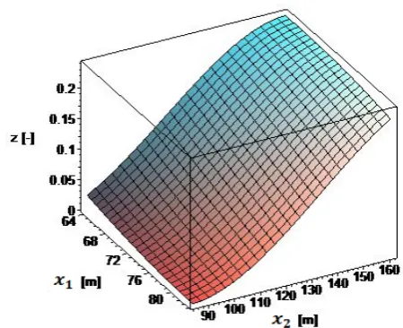
An explicit form of x is known and found in Refs. [1, 4]. The so-called p-factor, , is calculated on the basis of probability density distributions for relative damage location, penetration and length, given (a) longitudinal positions of transversal watertight bulkheads that define flooded compartment(s) and (b) the minimum breadth of flooding wing compartment(s). Fig. 1 shows how p-factor varies with positions of transversal bulkheads confining a damaged compartment. Apparently, the relationship is convex and the maximum p-factor value is when the bulkheads are farthest apart.

The ranges for and in Fig. 1 are taken from a simplified cruise ship subdivision with 22 transversal bulkheads shown in Fig. 2. We assume that the function topologies will not essentially be different in more complex subdivisions (e.g., with numerous longitudinal and stepped transfers bulkheads) and also ship types.

Note, the p-factor function for multiple compartment damages will have the same topological characteristics as for single compartment damage, but it will be additionally affected by intermediate (between and

) bulkhead positions as well [4]. The p-factor function for multiple compartment damages is of high dimensional and hence cannot be plotted for visual analysis. To this end, the p-factor function is seemingly convex, continuous and differentiable.

The missing link in understanding the topology of Eq. (2) is the s-factor, , which is the second element of component . Even though its explicit form is found in the regulations [1], that is

0.12

Range

16 . (3)

In Eq. (3), is a constant, is a maximum value of the positive righting lever, Range is the range of positive righting levers, both determined through hydrostatic stability calculations.

Fig. 1 The p-factor for single compartment, whose both ends are inside the ship length. Variables and are measured in meters from the aft terminal of the ship, hence defining the length and longitudinal position of the compartment.

Fig. 2 A reference model of a cruise ship1 with a simplified subdivision that is usually used in primary damage stability calculations. The required subdivision index is R = 0.83.

The s-factor relation to design variables such as bulkheads positions and is not necessary obvious. From the physical point of view, the s-factor must be a function of the size and the location of a flooded compartment (or a group of adjacent compartments). That is, the size of a flooded

1 _{Main particulars of the ship: length between particulars} Lbp =

293 m, length overall Loa = 323 m, breadth B = 36.8 m, design

compartment determines the volume of water that reduces the displacement of the damaged ship. In turn, the position of the flooded compartment tends to govern a combined effect of the heel and the trim on the ship’s stability. Thus, rather than using the coordinates of transverse watertight bulkheads and , we use the size and the position of a flooded compartment they define. That is,

, (4)

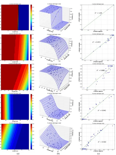
where is the size and is the position of the damage compartment or the group of adjacent compartments being flooded. Thus, Fig. 3a shows the contour plots of the s-factor function across different damage cases that involve one, two, three, four and five adjacent compartments (or zones) filled with water. The contour plots indicate, and this is also confirmed in Fig. 3b, that the s-factor function follows a sigmoidal shape, which is a continuous surface with large plateau of 1/0 values. From the physical point of view, the plateaux define areas of stability 1 or instability 0 for the damaged ship in term of the position and the size of the damage.

To this end, behavior of the s-factor is well defined. It ranges from 0 to 1 and resembles a Bernoulli trial with two dominating outcomes: survived 1

(success) and not survived 0 (failure). In statistics, this particular behavior of the dependent variable is well captured via the logistic regression (LR)2 [5], which has the following model.

x 1

1 exp x (5) where x is usually a linear model with the intercept defined as

x (6)

with being regression coefficients. In LR x

0,1 represents the probability of a particular outcome, given a set of explanatory variables x. This is exactly

2 _{Note, one of the properties of LR is that it can accommodate} heterogeneous variables in the model (6). That is, some variables can be continuous, other discrete or/and categorical. Thus for example, the compartment size and position can be given in frames (discrete), whereas can be given in meters (continuous).

what the s-factor represents: the probability of surviving a damage case described by design variables

 and and b; the latter being the minimum breadth of flooded wing compartment(s) when corresponding longitudinal bulkheads are present. The relevancy of LR is also backed by the fact that logistic function x in Eq. (5) is also sigmoidal. Thus, Eq. (5) can be rewritten as a regression model for the s-factor as

̃ ,, ,

1 1 exp

(7)

where is the vector of regression coefficients . Figs. 3b and 3c also shows application of LR on sample data for the s-factor. Specifically and interestingly, the approximation is very accurate for one and two compartment (zone) damages, and reasonably accurate for three, four and five compartment damages. Thus, the closer sample points to the sigmoidal shape, the more accurate regression results are. It’s important to note that regardless of the level of inconsistency between sample/calculated and regression points in Fig. 3, the expected value of the s-factor, , in both data sets is the same. That is, for each damage case model Eq. (8) holds when the number of samples is sufficiently large.

1

̃ ,, ,

of regression data

1

of sample data

(8)

where is the number of samples. Eq. (8) also holds for 57, which is the number of samples used in the plots of Fig. 3. Hence, the use of LR for approximating the s-factor can also be justified this way.

(a) (b) (c) Fig. 3 The variation of the s-factor function with the length and the position across multiple-zone damage cases: (a) a contour

involved in the damage case. The s-factor surface may exhibit large plateaux with 0/1 values where the function derivatives vanish. Therefore, the s-factor function may also be classified as a flat or locally constant function. Additionally, the s-factor function is non-convex, which stems from its sigmoidal shape.

Components of the subdivision index “A”, as defined in Eq. (2), are hence intersections of convex and non-convex sets that correspond to the p- and s-factor functions, respectively. As a result, components are non-convex functions of higher dimension. Consequently, the subdivision index “A” being a linear combination of non-convex functions is also a non-convex function of high dimension. For the strict convexity of a function implies the existence of just one maximum (or minimum) point, the non-convexity invalidates this theorem. Hence, the subdivision optimization problem such as studied in this work can have more than one global maximum.

3. Problem Complexity and Selection of

Optimization Strategy

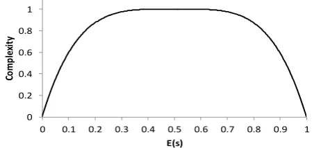
In this section we aim to formalize the complexity of the optimization problem. That is, bearing in mind the character of the p-factor and s-factor functions, it becomes obvious that the nonlinearity and irregularity in resulting functions of components is predominantly driven by the presence of large plateaux in s-factor functions. Thus, in case of some s-factors equal one, corresponding components represent a sum of differentiable and convex functions of the p-factors, which are hence easy to optimize. As s-factor decrease, components become irregular until they cease contributing to the subdivision index “A” when corresponding s-factors become zero. On this basis, we could define the complexity of the optimization problem to be proportional to the expected s-factor over all damage cases, E(s). The complexity vanishes when the expected s-factor value is either zero or one, thus forming a bell-shaped curve like the one in Fig. 4.

Fig. 4 Optimization complexity vs. expected survivability.

This brings us to the conclusion that the initial (prior to optimization) value of the index “A”, which by definition is the expected survivability, indicates how difficult the optimization of a ship subdivision is going to be. Specifically, the higher initial index “A”, the easier optimization algorithm will be able to improve the design, and vice versa. Certainty, various topological characteristics of the bell-shaped curve in Fig. 4 such as the inception the complexity descent and others will vary across different subdivision designs. However, this subject is beyond the scope of this paper.

As for the choice of an optimization method, deterministic gradient-based methods are definitely not applicable, unless the ship survives all the damages with the probability equal one. In this case the optimization of the index “A” would not be needed. Hence, we have no choice but to employ probabilistic (or stochastic) optimization methods that have been shown [6] to be suitable for this class of problems. Interestingly, probabilistic optimization methods and in particular genetic algorithms (GAs) [7] have been mainly applied in order to improve the index “A” [8-10]. However, the reason why GAs have been so popular is not because of anticipated problem complexity, but due to GA simplicity and hence convenience. This becomes obvious just observing the way the method has been used. That is, due to its stochastic nature, it should let run for an extended period of time3 _{to arrive at} solutions being close to the global optimum. However, since each evaluation of index “A” takes ca. 3.5 min for

3 _{A reasonable number of the index “A” evaluations can be} 1,000, which is a population of 10 individuals for 100 generations, neglecting the effect of mutation and crossover.

0 0.2 0.4 0.6 0.8 1

0 0.1 0.2 0.3 0.4 0.5 0.6 0.7 0.8 0.9 1

Co

m

pl

ex

it

y

Ro-Ro ships [9] and up to 20 min for cruise ships, to perform just 1,000 “A” evaluations it would take 58 and 333 hours, respectively. As this might be prohibitive in practice, such an extended optimization is not likely to be performed, satisfying with only some minor improvement. For all probabilistic methods in average having a similar performance [11], the same would also apply in case of using any other probabilistic method.

It stands to reason that the successful optimization of the index “A” requires an extensive exploration of design space. For this to happen, the runtime must be significantly reduced, to allow for numerous optimization runs. Such a reduction is only possible if we replace the time consuming hydrostatic calculations by approximate calculations. In other words, we need to find a surrogate function for the function behind the index “A” that is easy to implement and quick to evaluate. Such a surrogate function, which is based on the regression model from the preceding section, can be proposed to be as follows:

x x ̃ ,, , . (9)

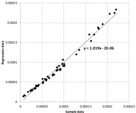
Note the s-factor in Eq. (9) represents the regression model of Eq. (7), whereas the p-factor is calculated according to the formulae described by the regulations [1, 4]. Interestingly to note, the p-factor can be also quite accurately approximated using the logistic regression model of Eq. (5) with independent variables corresponding to positions of all the p-factor affecting bulk heads. Thus for example, Fig. 5 shows a comparison of regression data with sample data for the p-factor for 5 zones damage case. The plot in Fig. 5 shows a good match even for 5 zones damage case, which involves 6 design variables (No. of zones + 1) affecting the p-factor. Thus, for fewer zones damage cases, the match should be even better.

Regardless the way the p-factor is estimated, it does not change the proposed optimization strategy at the heart of which is the use of the surrogate Eq. (9). The next section illustrates an application of the surrogate index “A” function to subdivision optimization.

Fig. 5 Regression vs. sample data of the p-factor for 5 zones damage case. Note, the slope (close to one-to-one match) and the intercept is negligible.

4. Surrogate Optimization of Index “A”

In this section we apply the surrogate index “A” Eq. (9) to optimize the subdivision shown in Fig. 2. First we summarize the process of deriving the regression-based surrogate function.

As for any other regression, we need to provide a data set based on which the regression coefficients can be estimated. The data can be sampled using some randomized sampling mechanism that should also be effective, in view of tedious calculations of the index “A”. We recommend the Latin hypercube sampling (LHS) [12] as an efficient sampling method that uniformly covers the design space. The number of samples in LHS is not required to increase with the number of variables that are subject to variation; this independence is one of the main advantages of this sampling scheme. Another advantage is that random samples can be taken one at a time, remembering which samples have been taken so far. In summary, the s-factor (and the p-factor analogically, if needed) is approximated according to the flowing procedure.

 The subdivision topology (number of bulkheads, tanks and openings) is fixed. This makes sure that the number of damage cases is the same for each run. This also implies that the subdivision topology must be optimized in advance, thus for instance, the optimal

y = 1.019x ‐2E‐06

0 0.00005 0.0001 0.00015 0.0002 0.00025

0 0.00005 0.0001 0.00015 0.0002 0.00025

Reg

res

si

o

n

da

ta

number of bu [13, 14].

 Genera prescribing r ranges shoul overlap. The N being the positions) to

 Run S subdivision contains all description ( case.

 Relate e design varia example, fou be related to a correspond

 Apply l estimate cor Eq. (6).

In the init the transvers

/

the last bulk transversal b longitudinal produced 57 them by (www.napa. for automate and logistic covering a q [0.883, 0.94 Further, w with index “ 17, 32 and them using Annealing ( difference in the optimiza

ulkheads can

ate subdivisio ranges of var ld be selected e recommend number of d o be optimized

SOLAS 20 alternative a damage cases (zones damag

each damage able through d

ur zones dam transversal bu ding longitudi

logistic regre rresponding

ial design of t sal bulkhead

1/2

kheads were bulkheads to

bulkheads 7 sample po naval arch fi). We used ed sampling, regression. F quite wide ran

] interval. we selected t

A” values of 47 in Fig. 6 the probabili (SA) [17]. I n which optim ation time wa

be found as d

n design alter riation for eac d in such a wa ded sample siz

esign variabl d.

09 calculat nd record the s with s-facto ged etc.) etc.

case, and hen damage descr age “Z3 / Z4 ulkheads TBH inal bulkhead

ssion for each regression c

the subdivisio equidistantly

2 . The first ( fixed and the

optimize wa were chosen oints via LH

hitecture so software plat

controlled d Fig. 6 shows t nge of index “

three worst d 0.888, 0.883 , respectively istic method In principle, mization meth as not limited

described in R

rnatives via L ch bulkhead. ay that they do ze is 3N [15] w les (e.g. bulkh

tions for e eir output, w or values, dam

per each dam

nce the s-facto riptions. Thus / Z5 / Z6” w H2 and TBH6 d between them

h damage cas coefficients β

on, we positio y, so that

from the aft) e total numbe as 20. Offsets n arbitrary. S and evalu oftware NA form spiral™ design evalua the sample po “A” values wi

design variat and 0.887 (po y) and optim

called Simul there was l hod was used d. We allowed

Refs. LHS, The o not with head each which mage mage or, to s for would 6 and m. se, to

β in

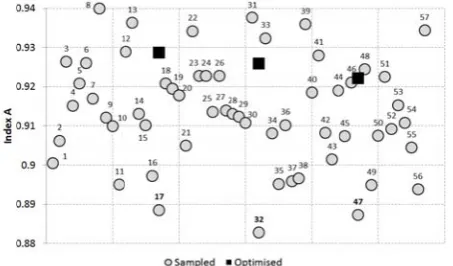
oned and er of s for We uated APA ™ [16] ation oints ithin tions oints mized lated little d, for d SA Fig. vari circ func inde

to r thre was opti corr imp (0.9 clea mea wel Hen surr eno solu T surr whi invo is n this read Vas

5. C

. 6 Index iations of subd cles are the v

ction. A label n ex.

run 10,000 f ee minutes), t s explored e

imization res responding 1 portant to not 929, 0.926, an arly inferior aning that the ll incorporate nce, even thou rogate Eq. (9 ough to find ution within t The apparent rogate model ich notably gr olved in a da needed to imp s is beyond th

der is referr ssalos [18].

Conclusion

t is generally blem is mu erwards. In ab

its understand

“A” (SOLAS division model variations opti next to a samp

function eva thus making extensively. sults in the fo

17, 32 and te that the fou

nd 0.922) are to some solu e surrogate fu e those superi ugh the optim 9) converged the relative g the given regi

t reason for lays in the re rows with the amage case. T prove the reg he scope of thi ed to a rela

ns

y accepted tha uch more di

bsence of a c ding, its solu

S 2009) value l in Fig. 2. Th imized using le point indica

luations (wh sure that the Fig. 6 also orm of three 47 sample und design im e significant, utions in the unction did no or designs in mization of the

well, it was global optim ion.

r this defici egression erro e number of c Therefore, fur gression mod is paper and t ated work b

at a proper de ifficult than correct proble ution is flawe

es for design he three black the surrogate ates the sample

hich took ca. design space o shows the black circles points. It is mprovements but they are e sample set, ot sufficiently n its structure. e constructed not accurate mum, i.e. best

iency in the or (see Fig. 3) ompartments rther analysis el. However, the interested y Puisa and

inefficient. This paper has shed light on the nature of the subdivision optimization problem (as implied by SOLAS 2009) with the aim to reducing uncertainty while selecting the most relevant optimization strategy.

In particular, we have performed topology analysis of the index “A” sub-functions and concluded that they are generally non-convex, multimodal (the presence of multiple maxima) and can be highly irregular with flat regions where the function derivatives vanish. The existence of large plateaux with s-factor values 0/1 also means that a Taylor series expansion, which is often employed by some gradient-based optimization algorithms, cannot be applied to the index “A” function, as there is no convergent infinite power series.

On this basis we have suggested that such irregularity of the index “A” function is reduced as the index increases. In other words, the higher the initial flooding survivability (i.e. the subdivision index “A”), the easier is to raise it further by optimizing positions of watertight bulkheads. This constitutes useful knowledge for practitioners who deal with the subdivision design problem on the regular basis.

Further, due to the highlighted irregularity of the index “A” function, optimization algorithms that require computation of derivatives are obviously irrelevant. Therefore, probabilistic methods such as genetic algorithms (GA) (or evolutionary algorithms in general), simulated annealing (SA) and other heuristics should be used instead. It is important to note that particularly because of the presence of the plateau and multiple function maxima, a selected probabilistic method must have mechanisms to handle these search impairing difficulties. Such mechanisms are usually related to diversity preserving strategies. Thus for example, the mutation probability in GA can be made adaptive, automatically increasing when the search stagnates and loses diversity [19]. In SA the cooling schedule can be made less steep/fast or/and the search can be restarted (resetting the initial temperature) when it starts stagnating.

We have also attempted to derive a surrogate

function for the index “A”, aiming to reduce the optimization time. The surrogate function is based on the logistic regression used to approximate the s-factor. The main reason to use the logistic regression for s-factor approximation was due to similarity between the topological shapes of the logistic function and the s-factor function. Specifically, the both functions follow the shape of a sigmoidal function. The logistic regression has proven to be a good way of approximating the s-factor, although the approximation error is present and it increases with the number of compartments involved in a damage case. We have tested the surrogate index “A” function in optimizing the subdivision of a cruise ship and found that its inaccuracy is detrimental, although the optimization results were feasible and represented significant improvement of initial designs. We hence conclude that the proposed surrogate model is generally unsuitable. It is worth reminding the reader that the approximation of the subdivision index “A” has not been an objective but rather a natural consequence of the analysis presented in this paper.

References

[1] MSC. 216 (82), Annex 2: Adoptation of amendmends to the international convention for the safety of life at sea, 1974, as amended, IMO, London, 2006.

[2] Z. Karaszewski, M. Pawłowski, A general framework of new subdivision regulations, in: Proceedings of the 8th International Marine Design Conference (IMDC), Athens, 2003, pp. 254-265.

[3] D. Cabaj, Floodable length surfaces as a novel approach to design of ship subdivision, Ph.D. Thesis, Deparment of Naval Architecture and Marine Engineering, University of Strathclyde, Glasgow, 2009.

[4] M. Pawlowski, Probability of flooding a compartment (the

pi factor)—A critique and a proposal, Engineering for the

Maritime Environment 219 (2005) 185-201.

[5] D.W. Hosmer, S. Lemeshow, Applied Logistic Regression, John Wiley and Sons, 1989.

[6] M. Gen, R. Cheng, Genetic Algorithms and Engineering Optimization (Engineering Design and Automation), John Wiley and Sons, 2000.

[8] E.K. Boulougouris, Optimization of arrangements of Ro-Ro passenger ships with genetic algorithms, Ship Technology Research 51 (2004) 99-105.

[9] A. Papanikolaou, Holistic ship design optimization, Computer-Aided Design 42 (2010) 1028-1044.

[10] A.İ. Ölçer, A hybrid approach for multi-objective combinatorial optimisation problems in ship design and shipping, Computers and Operations Research 35 (2008) 2760-2775.

[11] D.H. Wolpert, W.G. Macready, No Free Lunch Theorems for Search, Santa Fe Institute, 1995.

[12] R.L. Iman, An approach to sensitivity analysis of computer models, Part 1. Introduction, input variable selection and preliminary variable assessment, Journal of Quality Technology 13 (1981) 174-183.

[13] N. Tsakalakis, R. Puisa, D. Vassalos, Goal-based subdivision and layout, in: 10th International Conference on Stability of Ships and Ocean Vehicles, St Petersburg, Russia, 2009.

[14] G. Simopoulos, Sensitivity analsysis of the probabilistic damage stability regulations for RoPax vessels, Maritime Science and Technology 13 (2008) 164-177.

[15] R. Jin, Comparative studies of metamodeling techniques under multiple modeling criteria, Structural and Multidisciplinary Optimization 23 (2000) 1-13.

[16] R. Puisa, K. Mohamed, Prudent platform for multidisciplinary ship design exploration, analysis and optimisation, in: ICCAS 2011, International Conference on Computer Applications in Shipbuilding, Trieste, Italy, 2011.

[17] S. Kirkpatrick, Optimization by simulated annealing, Science 220 (1983) 671-680.

[18] R. Puisa, D. Vassalos, Surrogate optimisation of probabilistic subdivision index, in: Design and Operation of Passenger Ships Conference, London, 2011.