TRIANGULAR PRECONDITIONED BLOCK MATRICES
JENNIFER PESTANA†
Abstract. Block lower triangular matrices and block upper triangular matrices are popular preconditioners for 2×2 block matrices. In this note we show that a block lower triangular precondi-tioner gives the same spectrum as a block upper triangular precondiprecondi-tioner and that the eigenvectors of the two preconditioned matrices are related.
Key words. block triangular preconditioner, convergence, eigenvalues, eigenvectors, iterative method, saddle point system
AMS subject classifications. 65F08, 65F10, 65F50, 65N22
1. Introduction. Nonsingular block matrices of the form
A=
A BT
B −C
, (1.1)
where A ∈ Cn×n, B ∈ Cm×n with rank(B) = m, C ∈ Cm×m, m ≤ n arise in a
number of applications, many of which are discussed in the survey paper by Benzi, Golub and Liesen [5, Section 2]. Of particular interest are block matrices for which C= 0 and/or for whichAis symmetric positive definite andC is symmetric positive semidefinite [5],[10, Chapters 5 and 7].
In many applicationsAin (1.1) is large and sparse, in which case linear systems with A as the coefficient matrix are typically solved by a preconditioned iterative method. Two popular preconditioners are the block lower triangular matrix [8, 16, 17]
PL=
PA 0
B PS
, (1.2)
and block upper triangular matrix [6, 13, 15, 16, 20]
PU =
PA BT
0 PS
, (1.3)
wherePA∈Cn×n andPS ∈Cm×m(and, consequently,PL andPU) are nonsingular.
WhenAandCare Hermitian semidefinite it is known thatP−1
U AandP
−1 L Aare
similar [14, Remark 2]. (The case in which A is positive definite was also recently treated by Notay [16, Theorem 3.1].) For non-Hermitian matrices, Bai and Ng [3] analysed the minimal polynomials of P−1
L A and P
−1
U A when PA =A or PS is the
Schur complement, while Bai [1] obtained identical eigenvalue bounds forP−1 L Aand
P−1
U Ain the more general case of inexactPAandPS1. Additionally, Bai and Ren [4]
applied block triangular preconditioned GMRES [18] and BiCGStab [22] to nonsym-metric 2×2 block systems arising from discretizations of third-order ODEs. They
∗This publication is based on work supported by Award No. KUK-C1-013-04, made by King
Abdullah University of Science and Technology (KAUST).
†Mathematical Institute, University of Oxford, Andrew Wiles Building, Radcliffe Observatory
Quarter, Woodstock Road, Oxford, OX2 6GG, UK ([email protected])
1In fact the results of Bai and Ng [3] and Bai [1] are more general than ours since they do not
found that iteration counts for upper and lower triangular preconditioners were simi-lar, while eigenvalue plots forP−1
L AandP
−1
U Awere indistinguishable. Additionally,
for M-matrices arising from Markov chains Benzi and U¸car [7] noticed little differ-ence between the performances of block lower triangular and block upper triangular preconditioners.
In this note we extend the theoretical results to the non-Hermitian case. We show that PL−1AandPU−1A have identical spectra and relate the corresponding eigenvec-tors. WhenC= 0 andPL−1AandPU−1Aare diagonalizable, we bound the difference between the condition numbers of the eigenvector matrices; this gives some insight into when we might expect certain iterative methods to converge similarly for the block lower and block upper triangular preconditioned systems. Our results are illustrated on a numerical example.
Throughout Ip ∈ Cp×p denotes the identity matrix of dimension p and k · k2
represents the Euclidean vector norm or the corresponding induced matrix norm. The conjugate transpose of a matrixE is denoted by E∗, its range by range(E), its nullspace by null(E) and its Moore-Penrose pseudoinverse byE†.
2. Eigenvalue, eigenvector and condition number relationships. In this section we state our main results, starting with the equivalence of the spectra ofP−1
U A
andP−1 L A.
Proposition 1. LetA,PL andPU be invertible. Then the spectra ofPL−1Aand
P−1
U Aare identical, as are the spectra ofAP
−1
L andAP
−1 U . Proof. Let
Y(λ) =
A−λPA BT
(1−λ)B −(C+λPS)
and Z(λ) =
A−λPA (1−λ)BT
B −(C+λPS)
. (2.1)
Then the eigenvaluesλL of PL−1Amust be roots of det(Y(λL)) = 0 while the
eigen-valuesλU ofPU−1Amust satisfy det(Z(λU)) = 0. Setting
J(λ) =
In 0
0 (1−λ)Im
, (2.2)
we see that, for anyλ6= 1, 0 = det(Y(λL)) = det(J(λL)−1Y(λL)J(λL)) = det(Z(λL)).
Thus, the non-unit roots of det(Y(λ)) = 0 and det(Z(λ)) = 0 coincide. Additionally, det(Y(1)) = det(Z(1)) = (−1)mdet(A−P
A) det(C+PS). The results for right
pre-conditioning follow from the similarity ofP−1
L AandAP
−1
L and ofP
−1
U AandAP
−1 U .
The above result shows that if eigenvalues alone are important, there is nothing to distinguishP−1
L A,AP
−1 L ,P
−1
U AandAP
−1
U . This may be the case when, for example,
we precondition to achieve self-adjointness and positive definiteness with respect to a nonstandard inner product [8, 14, 17]. However, in many situations the eigenvectors will also have an effect on convergence. We relate the eigenvectors ofPL−1AandPU−1A in the following proposition.
Proposition 2. LetA,PL andPU be nonsingular.
1. Suppose thatλ6= 1is an eigenvalue ofPU−1A. If[uTU,vTU]T is the correspond-ing eigenvector, thenJ(λ)[uT
U,v T U]
T = [uT
U,(1−λ)v T U]
T is an eigenvector of
PL−1Acorresponding to this eigenvalue. 2. Suppose thatλ= 1 is an eigenvalue ofP−1
L A.
PA−1Athat corresponds to its unit eigenvalue. Moreover, the eigenvectors ofP−1
U Acorresponding to λare of the form[u T,((P
S+C)−1Bu)T]T.
• IfPA−Ais nonsingular then the eigenvectors ofPU−1Acorresponding to
λare of the form[0T,vT]T where v is any eigenvector of −P−1 S C that corresponds to its unit eigenvalue. Moreover, the eigenvectors ofP−1
L A corresponding toλare of the form[((PA−A)−1BTv)T,vT]T.
Proof. The first part follows immediately from Proposition 1, since ifλ6= 1 then Z(λ) =J(λ)−1Y(λ)J(λ) whereJ(λ) is as in (2.2).
Ifλ= 1, thenY(1)wL=0is equivalent to
AuL+BTvL=PAuL, (2.3)
PSvL+CvL=0, (2.4)
whileZ(1)wU =0is equivalent to
AuU−PAuU =0, (2.5)
BuU−CvU =PSvU. (2.6)
Note that −PS−1C does not have an eigenvalue at 1 if and only if PS +C is
nonsingular. In this case, (2.3) and (2.4) show thatvL=0and thatuL must be an
eigenvector ofPA−1A corresponding to the eigenvalue 1. Meanwhile, (2.5) and (2.6) implyuU 6= 0, since otherwise nonsingularity ofPS+C means thatvU = 0. Thus, uU is also an eigenvector of PA−1A corresponding to the eigenvalue 1 and BuU = (C+PS)vU.The last case is proved similarly.
Remark 1. The case thatλ= 1 is an eigenvalue of bothPA−1Aand−P
−1 S Ccan
also be worked out but is of less interest so we omit it here.
Remark 2. It may be preferable to use right preconditioning rather than left preconditioning, since doing so preserves the residual norm for methods such as GM-RES [18]. However, ifX is an eigenvector matrix ofP−1AthenPX is an eigenvector
matrix ofAP−1 for any invertible preconditioner P. This allows the eigenvectors of
the right preconditioned block matrix to be determined. However, the eigenvector matrices of AP−1
L and AP
−1
U do not have as straightforward a relationship as those
ofP−1
L AandP
−1
U Aand we do not consider them here.
Particularly important is the caseC= 0 inA, for which the eigenvectors ofP−1 L A
andP−1
U Aare more simply related.
Corollary 3. Let A,PL and PU be nonsingular and letC= 0 in (1.1). 1. Suppose thatλ6= 1is an eigenvalue ofPU−1A. If[uT
U,v T U]
T is the
correspond-ing eigenvector, then[uT
U,(1−λ)v T U]
T is an eigenvector ofP−1
L A correspond-ing to this eigenvalue.
2. Otherwise, λ= 1 is an eigenvalue of P−1
L A with corresponding eigenvector
[uT,0T]T, whereu is any eigenvector of the matrixP−1
A A that corresponds to its unit eigenvalue. Moreover, the eigenvectors ofP−1
U Acorresponding to
λare of the form[uT,(P−1 S Bu)
T]T.
Proof. IfC= 0, thenPS−1C= 0 and the last case in Proposition 2 does not apply.
Of interest for Krylov methods such as GMRES is the condition number of the eigenvector matrix [18] when it is invertible.
Corollary 4. Let A, PL and PU be nonsingular and let C = 0 in A. As-sume that both P−1
L A=XLΛXL−1 and P
−1
eigenvalues equal to 1, where
XU =
U(1) U(2) V(1) V(2)
andXL=
U(1) U(2) 0 V(2)(I−Λ(2))
, (2.7)
with U(1) ∈
Cn×p,U(2) ∈Cn×(n+m−p), V(1) ∈Cm×p, V(2) ∈Cm×(n+m−p) and Λ =
diag(Ip,Λ(2)),Λ(2) = diag(λp+1, . . . , λn+m). For any matrix E letPE = (I−EE†) andQE= (I−E†E)be orthogonal projectors ontonull(E)andnull(E∗), respectively. Then the 2-norm condition numbers κ2(XL)ofXL andκ2(XU)of XU are related by
1 α≤
κ2(XL)
κ2(XU)
≤α (2.8)
where, whenp= 0,
α= 1 +β 1 +kV(2)(I−Λ(2))(U(2))†k
2)
1 +β 1 +kV(2)(U(2))†k
2)
,
β =kV(2)Λ(2)k
2 k(U(2))†k2+kQU(2)(V(2))∗S−1k2
,
and whenp≥1
α= 1 +kV(1)(U(1))†k
2+kFk2β1 1 +kV(1)(U(1))†k2+kFk2β2,
β1=kG†k2+kH1†k2 1 +kV(2)(I−Λ(2))k2kG†k2
,
β2=kG†k2+kH2†k2 1 +kV(2)−V(1)(U(1))†U(2)k2kG†k2+kV(1)(U(1))†k2
.
Here, F =V(2)Λ(2)−V(1)(U(1))†U(2),G=P
U(1)U2, H1 =V(2)(I−Λ(2))QG,H2 =
(V(2)−V(1)(U(1))†U(2))Q
G andS=V(2)QU(2)(V(2))∗. Proof. It is clear from (2.7) thatXU =XL+K, where
K=
0 0
V(1) V(2)Λ(2)
.
From Ipsen [12, Corollary 3.3], we have that
σmax(XL)
σmax(XU)
≤1 +kKXU−1k2and
σmin(XU)
σmin(XL)
≤1 +kKXL−1k2, (2.9)
where σmax(X) = kXk2 and σmin(X) = 1/kX−1k2 are the largest and smallest
singular values ofX. Combining these results gives
κ2(XL)
κ2(XU)
≤(1 +kKX−1
U k2)(1 +kKX
−1
L k2). (2.10)
We now obtain expressions for KXL−1 and KXU−1, starting with the case p = 0. LetXL,U denote XL or XU as appropriate and let ˜V(2) =V(2) for XU and ˜V(2) =
V(2)(I−Λ(2)) forX
L. Then the inverse ofXL,UisXL,U−1 =XL,U∗ (XL,UXL,U∗ )−1, where
XL,UXL,U∗ =
I
n
˜
V(2)(U(2))† I
m
U(2)(U(2))∗ S
In ( ˜V(U(2))†)∗
withS = ˜V(2)Q
U(2)( ˜V(2))∗. SinceC = 0,PU−1AXU =XUΛ implies that V(2)Λ(2) =
PS−1BU(2). Thus, V(2)Λ(2)Q
U(2) = 0 and S = V(2)QU(2)(V(2))∗. Straightforward
calculation then yields
KXL,U−1 =
0 V(2)Λ(2)
(U(2))† Q
U(2)(V(2))∗S−1
I
n 0
−V˜(2)(U(2))† Im
and the upper bounds are obtained by bounding kKX−1
L k2 and kKXU−1k2. When
p≥1 we use Theorem 2.1 in Tian and Takane [21]. SinceU(1)has linearly independent
columns,QU(1) = 0, and
KXL−1=
0 0
V(1) V(2)Λ(2)
Ip −(U(1))†U(2)
0 In+m−p
(U(1))† 0 (I−H1†V(2)(I−Λ(2)))G† H†
1
=
0 0
V(1)(U(1))†+F(I−H†
1V(2)(I−Λ(2)))G† F H
†
1
.
Similarly, lettingN =V(2)−V(1)(U(1))†U(2),
KXU−1=
0 0
V(1) V(2)Λ(2)
Ip −(U(1))†U(2)
0 In+m−p
(U(1))† 0 (I−H2†N)G† H†
2
In 0
−V(1)(U(1))† I
m
=
0 0
V(1)(U(1))†+F[(I−H†
2(V(2)−V(1)(U(1))†U(2)))G†−H
†
2V(1)(U(1))†] F H
†
2
.
The upper bound on the condition number again follows from bounding the norms. Then, the lower bound on the condition number is achieved by boundingκ2(XU)/κ2(XL)
from above.
Although the expressions in Corollary 4 are quite complicated, they highlight that the difference between the condition numbers depends not only on the matrices that vary betweenXL andXU, namelyV(1),V(2)andV(2)(I−Λ(2)), but also on the
conditioning of U(1) and U(2). This is not surprising sinceU(1) and U(2) affect the conditioning ofXL andXU.
More specifically, when p= 0, αis smaller when k(U(2))†k
2 is small, i.e., when
U(2) is well conditioned in the sense that its smallest (nonzero) singular value is not
too small, and when the rows of V(2) are almost orthogonal to the rows ofU(2), so
that kV(2)(U(2))†k
2 is small. Also, since QU(2)(V(2))∗S−1 is a right inverse of V(2)
we expect its norm to be large when the rows ofV(2) are almost linearly dependent.
This confirms that well conditioned XL and XU and a small perturbation V(2)Λ(2)
ensure thatκ2(XL) andκ2(XU) are close.
Ifp >0,αdepends onkV(1)(U(1))†k
2,kFk2,β1andβ2. The termkV(1)(U(1))†k2
is small whenkV(1)k
2 is small but the smallest singular value ofU(1) is not.
Addi-tionally, kFk2 is small when kV(2)Λ(2)k2 and kV(1)k2 are small, and the columns
of U(1) are almost orthogonal to those of U(2). If range(U(2)) ⊂ range(U(1)), then G = 0, G† = 0, QG = I and a sufficient condition for β1 and β2 to be small is
that kV(2)(I −Λ(2))k
2, kV(2)k2 and kV(1)k2 are small. Otherwise, kG†k2 is not
too large if the columns of U(1) are orthogonal to those of U(2) with U(2) well conditioned. The terms H1 and H2 are the most difficult to analyse. Although
H1 = 0 when range((V(2)(I−λ(2)))∗)⊂range(G∗) and H2= 0 when range((V(2)−
V(1)(U(1))†U(2))∗)⊂range(G∗), these conditions may not hold in general. Alterna-tively, ifV(1)(U(1))†U(2)is small, a condition forH
1 andH2to be well conditioned is
Table 3.1
Left preconditioned GMRES iterations for the Stokes problem.
Grid IC AMG
PL PU PL PU
4×12 132 135 65 65 8×24 194 202 85 85 16×48 313 323 89 90 32×96 553 590 91 93
conditions together, we see that again α is small whenV(1) and V(2)Λ(2) are small in norm andXL andXU are well conditioned. We note that additional special cases
might also result in well conditioned matricesXL andXU and that Corollary 4 may
be useful for checking these.
Of course, neitherXU andXL, nor their condition numbers, are uniquely defined
(see, for example, the discussion in Bai, Benzi and Chen [2, Remark 3.1]). In our experiment we consider the eigenvector matrices for which each eigenvector has unit norm. To this end let us fix the columns [uT
i, vTi ]T,i= 1, . . . , n+m, ofXU in (2.7) to
have unit length, so thatkuik22+kvik22= 1. Then, the column scaling that transforms
XL to ˆXL, an eigenvector matrix with unit-length columns, is given by the diagonal
matrixD= diag(d11, . . . , dn+m,n+m), where
d−ii2=
(
1− kvik2, i≤p,
1 + (|λi|2−2<(λi))kvik2, i > p.
(2.11)
3. Numerical example. In our experience with incompressible Stokes and Navier-Stokes examples and preconditioners in IFISS [9, 19] and with time-harmonic Maxwell equations [11] we find, similarly to [4, 7], that there is often little difference between iteration counts achieved withPL−1Aand PU−1A. This seems to be true re-gardless of whether left or right preconditioning is used. However, there are certainly examples for which the condition numbers differ as we now show.
Our linear system comes from an incompressible Stokes problem that describes a flow over a backward facing step in two dimensions and is described in detail in Elman et al. [10, Example 5.1.2]. The equations are discretized byQ2−Q1finite elements in
Matlab using IFISS with default parameters. We apply left-preconditioned GMRES with a zero initial guess and terminate when the preconditioned residual decreases by eight orders of magnitude—although it may be desirable to consider the unprecondi-tioned residual, the precondiunprecondi-tioned residual is more closely connected with the theory of Section 2. In both of our preconditionersPS is the diagonal of the pressure mass
matrix. The first choice for PA is a no-fill incomplete Cholesky (IC) factorization
(produced by the Matlab commandichol) ofA0, the vector Laplace matrix obtained
with natural boundary conditions. The second is the algebraic multigrid (AMG) pre-conditioner implemented in IFISS. The eigenvector matrix XU is computed by the
Matlab functioneigwhileXLis computed fromXU using Corollary 3. BothXLand
XU are scaled to have unit-length vectors.
We first consider the incomplete Cholesky preconditioner. The eigenvalues of PL−1A(andPU−1A) lie in [−2.3,−0.046]∪[0.19,1.2]. Additionally, there are 20 eigen-values within 10−14 of 1 that we assume are unit eigenvalues. The iterations for
Table 3.2
Condition numbers of eigenvector matrices and norms of quantities in Corollary 4 for the problem on the8×24grid and the incomplete Cholesky preconditioner.
κ2(XL) κ2(XU) kV(1)k2 kV(2)Λ(2)k2 kV(1)(U(1))†k2 kFk2
23 54 2.1 6.4 10.6 6.5
kG†k2 kH1†k2 kH2†k2 kV(2)(I−Λ(2))k2 kV(2)−V(1)(U(1))†U(2)k2 α
[image:7.595.80.434.133.190.2]6.9 3.1 3.1 4.7 6.6 α= 8.8×10⁶
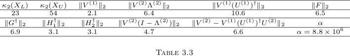
Table 3.3
Condition numbers of eigenvector matrices and norms of quantities in Corollary 4 for the problem on the8×24grid and the algebraic multigrid preconditioner.
κ2(XL) κ2(XU) kV(2)Λ(2)k2 kV(2)(U(2))†k2 kV(2)(I−Λ(2))(U(2))†k2
265 59 13.5 11.7 14.1
kSk2 α
1.6 α= 1.7×10⁷
is reflected in the condition numbers ofXL andXU (see Table 3.2). To further
in-vestigate the disparity in these condition numbers, we also list in Table 3.2 quantities related to Corollary 4. SincekXLk2 = 2.9 andkXUk2= 5.7, the perturbationsV(1)
and V(2)Λ(2) are relatively large in norm. Moreover, k(U(1))†k
2 = 9.1, so that U1
is not so well conditioned, and as a consequencekV(1)(U(1))†k
2 is large. Relative to
kV(1)(U(1))†k
2, the remaining terms in αare reasonably small and we conclude that
the most significant contributions to the difference betweenκ2(XL) and κ2(XU) are
U(1) and the perturbationsV(1) andV(2)Λ(2). We note that although the bounds in
Corollary 4 are not quantitatively descriptive for this problem they give insight into why the condition numbers ofXL andXU differ.
The eigenvalues of the AMG-preconditioned matrix lie in [−2.5,−0.01]∪[0.009,58] and no eigenvalue is within 10−14 of 1. The iteration counts appear to be
mesh-independent and are much lower than for the incomplete Cholesky preconditioner in spite of the wider distribution of eigenvalues (see Table 3.1). Additionally, PU−1A and PL−1A give similar iteration counts, with the latter performing slightly better for larger problems. Thus, the eigenvector condition numbers are not necessarily good predictors of convergence for this problem since, at least for the 8×24 grid, κ2(XL) > κ2(XU). Nevertheless, we can investigate why the condition numbers
differ by applying Corollary 4. Compared to kXLk2 = 4.5 and kXUk2 = 2.9,
kV(2)Λ(2)k
2 and k(U(2))†k2 = 20.6 are large. Consequently, kV(2)(U(2))†k2 and
kV(2)(I −Λ(2))(U(2))†k
2 are large relative to the other terms in α. From this we
deduce that the norm of (U(2))† and the size of the perturbation V(2)Λ(2) are the
main causes of the difference betweenκ2(XL) andκ2(XU).
For this problem the condition number bound (2.8) overestimatesκ2(XU)/κ2(XL).
We note that there are other examples for which (2.8) is tight—these are typically problems for whichκ2(XU) and κ2(XL) are close. When the difference between the
condition numbers increases, the bound (2.8) is usually not as tight, with (2.10) over-estimatingκ2(XU)/κ2(XL) and the subsequent bounds onkKXU−1k2 andkKXL−1k2
then causing (2.10) to be overestimated.
4. Conclusion. In summary, when the eigenvalues are important, or when the eigenvector matrices XL and XU are fairly well conditioned, there is no benefit in
choosing PL over PU or vice versa. (Note that since the eigenvector matrix is not
uniquely defined, the conditioning could be related to the particular choice of matrix.) We have shown that the eigenvectors of P−1
L A and P
−1
and this can affect the condition numbers of the eigenvector matrices (when P−1 U A
and P−1
L A are diagonalizable). However, the convergence rate of GMRES remains
weakly sensitive to these factors for the problems examined, and for others in the the literature. WhenC= 0 and P−1
L A andP
−1
U Aare diagonalizable, we can bound the
ratio of the condition numbers of the eigenvector matricesXLandXU, which depend
not only on difference betweenXLandXU, contained inV(1) andV(2)Λ(2), but also
onU(1) andU(2).
Acknowledgments. The author would like to thank the editor and referees, who offered many helpful comments and suggestions, and Yvan Notay, whose manuscript on symmetric saddle point matrices inspired this work.
REFERENCES
[1] Z.-Z. Bai,Structured preconditioners for nonsingular matrices of block two-by-two structures, Math. Comp., 75 (2006), pp. 791–815.
[2] Z.-Z. Bai, M. Benzi, and F. Chen,On preconditioned MHSS iteration methods for complex symmetric linear systems, Numer. Algorithms, 56 (2011), pp. 297–317.
[3] Z.-Z. Bai and M. K. Ng,On inexact preconditioners for nonsymmetric matrices, SIAM J.
Sci. Comput., 26 (2005), pp. 1710–1724.
[4] Z.-Z. Bai and Z.-R. Ren, Block-triangular preconditioning methods for linear third-order ordinary differential equations based on reduced-order sinc discretizations, Japan J. In-dust. Appl. Math., 30 (2013), pp. 511–527.
[5] M. Benzi, G. H. Golub, and J. Liesen,Numerical solution of saddle point problems, Acta
Numer., 14 (2005), pp. 1–137.
[6] M. Benzi, M. A. Olshanskii, and Z. Wang,Modified augmented Lagrangian preconditioners for the incompressible Navier-Stokes equations, Int. J. Numer. Meth. Fluids, 66 (2011), pp. 486–508.
[7] M. Benzi and B. Uc¸ar,Block triangular preconditioners for M-matrices and Markov chains, ETNA, 26 (2007), pp. 209–227.
[8] J. H. Bramble and J. E. Pasciak,A preconditioning technique for indefinite systems resulting from mixed approximations of elliptic problems, Math. Comp., 50 (1988), pp. 1–17. [9] H. C. Elman, A. Ramage, and D. J. Silvester,Algorithm 866: IFISS, a Matlab toolbox for
modelling incompressible flow, ACM Trans. Math. Software, 33 (2007). Article 14. [10] H. C. Elman, D. J. Silvester, and A. J. Wathen,Finite Elements and Fast Iterative Solvers:
with applications in incompressible fluid dynamics, Oxford University Press, Oxford, 2005. [11] C. Greif and D. Sch¨otzau,Preconditioners for saddle point linear systems with highly
sin-gular(1,1)blocks, Electron. Trans. Numer. Anal., 22 (2006), pp. 114–121.
[12] I. C. F. Ipsen,Relative perturbation results for matrix eigenvalues and singular values, Acta Numer., 7 (1998), pp. 151–201.
[13] ,A note on preconditioning nonsymmetric matrices, SIAM J. Sci. Comput., 23 (2001), pp. 1050–1051.
[14] A. Klawonn,Block-triangular preconditioners for saddle point problems with a penalty term, SIAM J. Sci. Comput., 19 (1998), pp. 172–184.
[15] M. F. Murphy, G. H. Golub, and A. J. Wathen,A note on preconditioning for indefinite
linear systems, SIAM J. Sci. Comput., 21 (2000), pp. 1969–1972.
[16] Y. Notay,A new analysis of block preconditioners for saddle point problems, SIAM J. Matrix Anal. Appl., To appear (2013).
[17] J. Pestana and A. J. Wathen, Combination preconditioning of saddle point systems for positive definiteness, Numer. Linear Algebra Appl., 20 (2013), pp. 785–808.
[18] Y. Saad and M. H. Schultz,GMRES: a generalized minimal residual algorithm for solving nonsymmetric linear systems, SIAM J. Sci. Stat. Comput., 7 (1986), pp. 856–869. [19] D. J. Silvester, H. C. Elman, and A. Ramage,Incompressible Flow and Iterative Solver
Software (IFISS) version 3.1, January 2011. http://www.manchester.ac.uk/ifiss/. [20] V. Simoncini,Block triangular preconditioners for symmetric saddle-point systems, Appl.
Nu-mer. Math, 49 (2004), pp. 63–80.