A 'dipper' function for texture discrimination based on orientation variance

A

‘

dipper

’

function for texture discrimination based

on orientation variance

Department of Optometry, City University London, UK

Michael

Morgan

Department of Cognitive Sciences, University of California, Irvine, USA

Charles

Chubb

Department of Optometry, City University London, UK

Joshua A.

Solomon

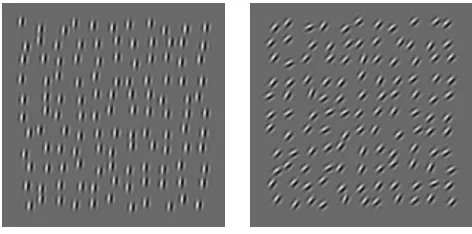
We measured the just-noticeable difference (JND) in orientation variance between two textures (Figure 1) as we varied the baseline (pedestal) variance present in both textures. JND’s first fell as pedestal variance increased and then rose, producing a‘dipper’function similar to those previously reported for contrast, blur, and orientation-contrast discriminations. A dipper function (both facilitation and masking) is predicted on purely statistical grounds by a noisy variance-discrimination mechanism. However, for two out of three observers, the dipper function was significantly betterfit when the mechanism was made incapable of discriminating between small sample variances. We speculate that a threshold nonlinearity like this prevents the visual system from including its intrinsic noise in texture representations and suggest that similar thresholds prevent the visibility of other artifacts that sensory coding would otherwise introduce, such as blur.

Keywords: visual acuity, computational modeling, learning, middle vision, texture

Citation:Morgan, M., Chubb, C., & Solomon, J. A. (2008). A‘dipper’function for texture discrimination based on orientation variance.Journal of Vision, 8(11):9, 1–8, http://journalofvision.org/8/11/9/, doi:10.1167/8.11.9.

Introduction

The nervous system is noisy and all sensory signals are subject to perturbation (Barlow, 1981). Studies of ori-entation classification (Dakin,1999; Dakin & Watt,1997; Morgan,1990) suggest that the visual system perturbs the orientations of individual elements with a variance of approximately 1 deg. There is a problem, then, in understanding why we do not see orientation variance in a texture composed of parallel elements, like that on the left-hand side of Figure 1. If the internally represented orientation of each element were independently sampled from a Gaussian distribution, then all the elements should look different, even if they are physically parallel. In an array of 121 elements (Figure 1) it would not be at all unlikely that a particular element would have an apparent orientation 2Afrom its true value. A possible resolution of this paradox is that when we see a texture as uniform, we are not seeing the orientation of every element in the texture, but rather the output of a specialized mechanism that computes orientation variance. If stimulation of this mechanism were subject to a threshold nonlinearity, then the perceived uniformity of a uniform texture could be explained.

A threshold would be useful for eliminating early noise from mid-level visual representations. The idea that sensory systems discount their own imperfections is suggested by the absence of sensory hallucinations in everyday life, and from the apparent sharpness of the

retinal image. In reality, the retinal image is considerably blurred by imperfections in the optics, and by inescapable diffraction through a small pupil, but we become conscious of this blur only when it exceeds normal levels, for example, when we need spectacles. The idea that blur is detected only when it exceeds a threshold is supported by studies of blur discrimination, both in stationary (Georgeson,1994; Watt & Morgan,1983) and in moving images (Burr,1980,1981; Burr & Morgan,1997; Morgan & Benton, 1989; Paakkonen & Morgan, 1993). Blur discrimination thresholds between two patterns have a characteristic ‘dipper’ shape similar to that for contrast discrimination (Nachmias & Sansbury, 1974). As small amounts of blur are added to both images, the just-noticeable difference (JND) in blur first falls, and then rises again. The initial fall would be expected from a threshold, since a small amount of blur would raise the response of the mechanism to just below the threshold, making an additional increment easier to see. The rise in JND at even higher pedestal levels, referred to as ‘masking’, is usually explained by a compressive non-linearity (Foley,1994; Legge & Foley,1980; Ross, Speed, & Morgan, 1993), or alternatively by multiplicative sensory noise (Solomon,2007).

mainly interested in the masking region, where JND’s increased with the pedestal contrast, Motoyoshi and Nishida also noted facilitation at small, nonzero pedestal contrasts. That is, they found that JND’s formed a dipper function of pedestal contrast.

Facilitation at small, nonzero luminance contrasts is normally taken as evidence for a threshold nonlinearity (e.g., Foley & Legge, 1981; Legge & Foley, 1980). However, in the case of variance discrimination, facili-tation is expected simply on the basis of intrinsic noise (Laming, 1986; Paakkonen & Morgan, 1993).1 The full derivation is given in the Appendix A, but the informal argument runs thus. Suppose, in a 2AFC experiment, the observer compares two sample variances, each of which reflects the visual system’s internal noise as well as the stimulus variance. The function mapping stimulus var-iance to sample varvar-iance will thus have two distinct parts; a flat part, in which the stimulus variance is negligible compared to the internal noise, and a steadily increasing part, in which the internal noise is negligible. Because of the flat part, any criterion increase in sample variance will require a larger increase in stimulus variance when sample variance is low.

The Appendix A shows that dipper functions are predicted even for an ideal observer who compares sample variances, whether or not there is an additional threshold nonlinearity. We wished to determine whether the addition of a sensory threshold would significantly improve the ideal observer’s fit to variance discriminations.

Methods

In addition to the extensive observations undertaken by three experienced observers, a shorter series was com-pleted by four psychophysically practiced observers who did not know the purpose of the experiment. Apart from

noting that all of these observers showed facilitation (i.e. a ‘dip’), we do not report the latter group’s data further.

Stimuli were presented on the LCD screen of a Sony Vaio (PGC-TR5MP) laptop computer using MATLAB and the PsychToolbox (Brainard, 1997) for Windows. Screen size was 1280768 pixels (230140 mm). Only the Green LCD’s were used, and the mean luminance was 56 cd/m2. The viewing distance was approximately 57 cm so that the pixel size was approximately 0.018 deg of visual angle. The texture elements were Gabor wavelets of maximum contrast. Specifically, the Weber contrast g

varied as a function of position x, y with respect to the center of the wavelet as follows:

g xð ;y;EÞ ¼exp jx

2 Eþy2E

2A2

sin 2:xE

1

; ð1Þ

where 1 (the wavelength of the windowed grating) is 0.1198 deg, A (the space constant of the window) is1/2, andEgives the angle normal to grating orientation; that is,

xE ¼xcosðEÞ þysinðEÞ; ð2Þ

and

y_E ¼jxsinðEÞ þycosðEÞ; ð3Þ

The elements were laid out in an 11 11 lattice with spacing 31,slightly perturbed by displacing each elements randomly in xandy by an amount drawn from a uniform pdf with width 1.51. Thus, the whole array subtended approximately 3.6 deg of visual angle. The jitter was resampled between each of the two stimulus presentations on every trial.

On each trial two textures like those in Figure 1 were shown, each for 200 msec and with a 200-msec blank interval in between. Element orientations E were drawn from Gaussian probability density functions. For one of the two textures, the density had random mean and “pedestal” varianceAp2. The density for the other texture had a different random mean and greater variance (Ap + $A)2. The mean orientation was randomized between presentations, to prevent the use of any one orientation-tuned channel by the observer, and spatial position of the elements was jittered between presentations.

The QUEST procedure (Watson & Pelli, 1983) adap-tively determined the JND$A at which the observer was 82% correct. There was no feedback to indicate whether the response was correct or not. The pedestal variance was randomly selected on each trial from a set of preset values. A block of trials terminated when each of these preset values had been presented 50 times. Thus, when

ApZ{0-, 1-, 2-, 4-, 8-, 16-}, as was the case for observers MM (6 blocks) and JAS (9 blocks) and IM (4 blocks), each block contained 300 trials. The four naive observers

experienced only one block, with interleaved pedestal levels {0-, 1-, 2-, 4-} only.

Confidence limits (95%) for the JND were determined by exactly simulating the experiment 80 times with a bootstrapping procedure (Efron,1982).

Results

Results (Figure 2) showed clear evidence for a ‘dipper.’ JND’s were comparatively high when one of the patterns had no variance (the leftmost point on the graphs) and fell as variance was added. The curves inFigure 2 show the best fits to the data. (Note that these are not fits to the data points in the graph but are rather maximum likelihood fits (found with the FMINSEARCH function of MATLAB) of the model to data vectors consisting of the pedestal level,

added signal level, and observer’s response on every trial of the experiment.) These best-fitting parameter values and their associated log likelihoods are shown inTable 1.

Aint n+ 1 c ln L

MM no thresh 2.87 9 – j647.10

MM + thresh 2.23 8 3.16 j642.11**

IM no thresh 2.49 5 – j504.83

IM + thresh 0.98 4 2.86 j495.91**

JAS no thresh 4.80 10 – j1010.6

JAS + thresh 4.82 9 1.04 j1010.6 (NS)

Table 1.Bestfitting values for intrinsic noiseAint, number samples n + 1, sensory thresholds c, and log-likelihoods (ln L) for three observers (MM, IM, and JAS). The models are described in the Appendix A. The asterisks show when the threshold model is a significantly betterfit (pG.01) than the nonthreshold model.

A likelihood ratio test was used to compare the fits of the two models, one with and one without a threshold. Let

LCandLUbe the likelihoods of the best-fitting constrained and unconstrained models. As is well-known (e.g., Hoel, Port, & Stone, 1971), under the null hypothesis that the constrained model captures the true state of the world,

X¼j2ln LC

LU ; ð4Þ

is asymptotically distributed as chi-square with 1 degree of freedom (for the single additional free parameter inLU). The chi-square values were significant (p G .010) for observers MM and IM, but not for observer JAS. To give a more intuitive impression of the success of the two models,Figure 3 plots the relative likelihoods in compar-ison to two extreme baselines. The ‘coin flipping’ model has the simulated observer choose between the two intervals with equal probability, independently of the stimulus level or pedestal. This is as poor as a fit could be. The ‘Weibull fits’ model shows the best fit of a set of 2-parameter Weibull psychometric functions to the each of the pedestal conditions separately. This model has 2n

free parameters, where n is the number of pedestals, in comparison to the 2 and 3 parameters of the models described in Table 1, and it is as good as a fit could be given the noise in the observer’s data. It is satisfying to see that the models are much closer to the Weibull fits than to ‘coin flipping’. The two versions of the intrinsic noise model, with and without an additional threshold, are seen to be very close.

Finally, to see if the threshold nonlinearity giving rise to the dipper was modifiable by experience, one observer (MM) undertook an extensive series of observations with

a zero pedestal to see if performance would improve. Results (shown inFigure 4) failed to find any evidence for learning.

Discussion

We consider possible explanations for the dipper function found in our experiments.

Intrinsic noise

Intrinsic noise produces a dipper function for variance discrimination (see Appendix A). Both the initial fall and subsequent increase in JND (Weber’s Law) arise because variance discrimination is necessarily a second-order computation. In a first-order computations, such as mean discriminations, intrinsic noise typically produces a flat region of the graph of JND vs. noise (e.g., Mansouri, Allen, Hess, Dakin, & Ehrt,2004). On the other, hand, we expect, and find, a dipper function for contrast discrim-ination of orientation- and contrast-modulated gratings (Kingdom, Prins, & Hayes, 2003) and of dynamic visual noise (Morgan, McEwan, & Solomon, 2007). Blur discrimination is another clear case where there is a dipper (see Introduction) and where a case can be argued for its being a special case of variance discrimination in the luminance domain. The variance of point-luminance values across a sharp edge is different from that across less sharp edge; and indeed, Watt and Morgan (1983)

Figure 3.The bars in thefigure show relative likelihoods (different absolute scales of log likelihood for each observer) for the signal-detection model of variance discrimination (pink bars) and for the same model supplemented by a threshold (blue bars). The labeled horizontal lines show the likelihoods of a coin-flipping model and of separate Weibullfits to the data at each pedestal value. For further explanation, see the text.

produced their blurred edges by convolution of a step with a specified blurring function, defined by its variance.

Internal noise with a sensory threshold

Our results show qualitative agreement with the intrinsic noise model, but for all three observers the extent of facilitation is greater than predicted by the model. For two of the observers, the data were better fit by a model in which there is both internal noise and a threshold. The existence of a threshold could explain why we do not see the internal noise in a completely regular texture like that on the left ofFigure 1. There are good reasons why the visual system should not represent its own noise when computing the variance of a pattern in the outside world, and there is collateral evidence that such thresholding happens in the case of blur, both of stationary and moving objects. The effect of the threshold will be to make textures appear slightly more regular than is in fact the case and this bias could be interpreted as a Bayesian prior in favor of seeing regularity in the world (Schwartz, Sejnowski, & Dayan,2006). We admit, however, that this interpretation is entirely speculative, and that we do not have data that exclude other models.

Consistent with our current finding is previous work demonstrating an inability to extract local estimates of orientation from briefly glimpsed ‘crowded’ arrays when the regional orientation variance is small (Parkes, Lund, Angelluci, Solomon, & Morgan,2001). Solomon, Felisberti, and Morgan (2004) noted this latter result implied that individual elements should appear more aligned than they really were and formulated a model wherein this ‘small-angle assimilation’ was the result of lateral amplification between neurons with the same orientation preference. (That model also contained a stronger, more broadly tuned, lateral inhibition, which produced repulsion when orienta-tion variance was larger.) Lateral amplificaorienta-tion may under-lie the sensory threshold manifest in our present results, but once again this is pure speculation. To make a stronger connection between small angle assimilation and the dipper function would require measurement of the dipper function in crowded displays.

Channel uncertainty

A different interpretation of the ‘dipper’ for contrast discrimination is that it reflects intrinsic uncertainty, which the observer has about the best channel to use when making the discrimination (Pelli, 1985). When the pedestal is zero, there are many channels the observer could monitor, each with a level of intrinsic noise. It is therefore likely that noise in one of the channels will masquerade as a signal. With a nonzero pedestal, how-ever, the response in the channel most responsive to the signal will be elevated to a point where noise in other

channels will be unlikely to exceed it. This model accounts well for many facts about contrast discrimina-tion, but we find it difficult to see how it applies in the case of orientation variance discrimination. As far as orientation-tuned channels are concerned, the essence of our procedure was to ensure that the observer could not do the task by monitoring selected channels. Recall that the mean orientation of the stimuli was randomized both over trials and between the two stimuli in the 2AFC task. Thus, there was no information about variance to be derived from a single channel. The only way we can see to make an uncertainty model work is if there are different channels corresponding to different levels of variance. This is the possibility we consider next.

Multiple channel models of variance discrimination

Wavelength discrimination shows notches in certain regions of the spectrum, where there is a local minimum in the JND. The explanation is thought to be, in part, that these are regions where the difference in quantum catch of the L, M, and S cones is greatest as wavelength changes (Wyszecki & Stiles, 1967). It would be possible to envisage a similar model for variance discrimination, with one mechanism selectively but widely tuned to low variance, and another to a higher variance (Thompson,

1984). If there are such channels they should be revealed by selective adaptation.

Conclusion

The most parsimonious explanation of the dipper function for orientation variance is that it is produced by intrinsic noise in a specialized mechanism for variance computation. Our findings argue caution before automati-cally ascribing dippers, such as those for blur discrim-ination, to a threshold nonlinearity. However, we cannot rule out the possibility that there is an additional thresh-old, at least in two of our observers. Further investigations of the population are required to see whether there are genuine individual differences in this respect.

Appendix A

Signal-detection theory for variance discrimination

smaller varianceAp 2

. The model observer collects a sample of sizen + 1 from the first interval, a sample of the same size from the second interval, and responds correctly when the variance of the former sample exceeds that of the latter. These two sample variances can be denoted by the independent random variables S and N, respectively. The expected response accuracy is given by the formula

P Cð Þ ¼P Sð 9NÞ ¼

Z _V

jVFNð Þx fSð Þx dx

¼ Z _V

0

FNð Þx fSð Þx dx; ðA1Þ

whereFN(x) is the cumulative distribution function (CDF) ofN, and fS(x) is the probability density function (PDF) ofS. The lower limit of integration is zero because neither

SnorN can ever be negative.

Allowing internal noise

Consider what happens when each element of each sample is perturbed by internal Gaussian noise with zero mean and varianceAint2 . In that case,Swill be [(Ap+$A)2+

Aint2 ]/(n + 1) times a chi-square random variable (call it

U), having n degrees of freedom; and N will be (Ap2 +

Aint2 )/(n + 1) times an independent chi-square random variable (call itV), also havingn degrees of freedom; and probability correct is given by the formula

P Cð Þ ¼P U

Apþ$A

2

þA2 int

h i

nþ1 9V

Ap2þA2int

nþ1

0 @

1 A

¼P U

V 9

Ap2þA2int Apþ$A

2

þA2 int

!

¼1jF Ap

2_þA2 int Apþ$A

2

þA2 int

" #

; ðA2Þ

where F is the F-distribution, with degrees of freedom

nandn.

Also allowing a sensory threshold

This simple formula (Equation A2) cannot be used when we allow a sensory threshold, but note that iffX(x;n)

andFX(x;n) are the PDF and CDF for a chi-square random

variableX,withndegrees of freedom; thenfX(x/a;n)/aand

FX(x/a;n) will be the PDF and CDF for aX, as long as a 90. Therefore, the CDF for Ncan be written as

FNð Þ ¼x FX xðnþ1Þ= Ap2þA2int

;n

; ðA3Þ

and the PDF and CDF forS are

fSð Þ ¼x

fX x½nþ1

.

Apþ$A

2

þA2 int

h i

;n

ðnþ1Þ

Apþ$A

2

þA2

int ðA4Þ

and

FSð Þ ¼x FX x½nþ1

.

Apþ$A

2

þA2 int

h i

;n

: ðA5Þ

Now consider what happens when there is a sensory threshold c, below which all sample variances are indistinguishable from zero. Either the sample variance from the first interval (the one with the larger variance) could be bigger than that from the second interval, or neither sample variance could exceed the threshold and the observer makes a lucky guess. Therefore, the expected response accuracy for 2AFC would be

P Cð Þ ¼P Sð Qc; S9NÞ þ1

2P Sð Gc; NGcÞ

¼ Z _V

c

FNð Þx fSð Þx dxþ

1

2FNð Þc FSð Þ:c ðA6Þ

Weber’s Law

In this final section, we argue that 2AFC responses based on sample variance automatically produce Weber’s Law, a consequence first noted by Green and Swets (1966). The only constraint is that the stimuli only vary in variance. That is, if the CDF of stimulus values FX(x), is

such that

FXð Þ ¼x F x=

ffiffiffiffiffiffiffiffiffiffiffi

varX

p

h i

OX; ðA7Þ

then it can be shown that

F_S2

Xð Þ ¼x FS

2½x=varX; ðA8Þ

where FS2

X(x) is the CDF of SX

2_{, the sample variance ofX,} and FS2 (x) is the CDF of S2, a same-sized sample of

To obtain the expected response accuracy, we can set

y= x/varS, and substitute into Equation A1:

P Cð Þ ¼

Z _V

0 FS2

varS

varNy

fS2ð Þy dy: ðA9Þ

Let us assume that the pedestal is sufficiently large so that we can forget about the internal noise and any sensory threshold (i.e.Ap2d Aint2,c). In that case,

P Cð Þ ¼

Z _V

0

FS2 y 1þ$A Ap

2

" #

fS2ð Þy dy: ðA10Þ

That is, the expected response accuracy is purely a function of$A/Ap. This is Weber’s Law.

Acknowledgments

We would like to thank David Burr for encouragement, Marc Ernst for suggesting that intrinsic noise could masquerade as a sensory threshold, Beau Watson for remembering Paakkonen & Morgan, and Ahna Girshick for suggesting Figure 3 in her 2008 VSS talk. Supported by a Grant from the EPSRC.

Commercial relationships: none.

Corresponding author: Michael Morgan. Email: m.morgan@city.ac.uk.

Address: Department of Optometry, City University London, Northampton Square, London, EC1V 0HB, UK.

Footnote

1_{Paakkonen and Morgan (1993) assumed that two}

blurred edges were discriminated as a function of the difference in their internally represented blur, which combined extrinsic and intrinsic blur by convolution (Equation 6 of their paper). However, they assumed Weber’s Law rather than deriving it from sampling as we do in this paper.

References

Barlow, H. B. (1981). The Ferrier Lecture, 1980. Critical limiting factors in the design of the eye and visual cortex. Proceedings of the Royal Society of London B: Biological Sciences, 212, 1–34. [PubMed]

Brainard, D. H. (1997). The Psychophysics Toolbox.

Spatial Vision, 10, 433–436. [PubMed]

Burr, D. C. (1980). Motion smear. Nature, 284,164–165. [PubMed]

Burr, D. C. (1981). Temporal summation of moving images by the human visual system. Proceedings of the Royal Society of London B: Biological Sciences, 211,321–339. [PubMed]

Burr, D. C., & Morgan, M. J. (1997). Motion deblurring in human vision. Proceedings of the Royal Society B: Biological Sciences, 264,431–436. [PubMed] [Article] Dakin, S. C. (1999). Orientation variance as a quantifier of structure in texture. Spatial Vision, 12, 1–30. [PubMed]

Dakin, S. C., & Watt, R. J. (1997). The computation of orientation statistics from visual texture. Vision Research, 37,3181–3192. [PubMed]

Efron, B. (1982). The jackknife, the bootstrap and other resampling plans. Philadelphia: Society for Industrial and Applied Mathematics.

Foley, J. M. (1994). Human luminance pattern-vision mechanisms: Masking experiments require a new model. Journal of the Optical Society of America A, Optics, Image Science, and Vision, 11, 1710–1719. [PubMed]

Foley, J. M., & Legge, G. E. (1981). Contrast detection and near-threshold discrimination in human vision.

Vision Research, 21,1041–1053. [PubMed]

Georgeson, M. A. (1994). From filters to features: Location, orientation, contrast and blur. In G. R. Bock & J. Goode (Eds.), Higher-order processing in the visual system. Chichester: Wiley.

Green, D. M., & Swets, J. A. (1966). Signal detection theory and psychophysics(1st ed.). New York: Wiley. Hoel, P. G., Port, S. C., & Stone, C. J. (1971).

Introduction to statistical theory. Boston: Houghton Mifflin.

Kingdom, F. A., Prins, N., & Hayes, A. (2003). Mecha-nism independence for texture-modulation detection is consistent with a filter-rectify-filter mechanism.

Visual Neuroscience, 20,65–76. [PubMed] Laming, D. (1986). Sensory analysis: Academic Press. Legge, G. E., & Foley, J. M. (1980). Contrast making in

human vision. Journal of the Optical Society of America, 70,1458–1471.

Mansouri, B., Allen, H. A., Hess, R. F., Dakin, S. C., & Ehrt, O. (2004). Integration of orientation information in amblyopia. Vision Research, 44, 2955–2969. [PubMed]

Morgan, M. J. (1990). Hyperacuity. In D. Regan (Ed.),

Spatial vision (pp. 87–113). London: Macmillan. Morgan, M. J., & Benton, S. (1989). Motion-deblurring in

Morgan, M. J., McEwan, W., & Solomon, J. (2007). The lingering effects of an artificial blind spot.PloS ONE, 2, e256. [PubMed] [Article]

Motoyoshi, I., & Nishida, S. (2001). Visual response saturation to orientation contrast in the perception of texture boundary. Journal of the Optical Society of America A, Optics, Image Science, and Vision, 18,

2209–2219. [PubMed]

Nachmias, J., & Sansbury, R. V. (1974). Letter: Grating contrast: Discrimination may be better than detection.

Vision Research, 14,1039–1042. [PubMed]

Paakkonen, A., & Morgan, M. J. (1993). The effects of motion blur on blur discrimination. Journal of the Optical Society of America A, Optics, Image Science, and Vision, 11, 992–1002.

Parkes, L., Lund, J., Angelucci, A., Solomon, J. A., & Morgan, M. (2001). Compulsory averaging of crowded orientation signals in human vision. Nature Neuroscience, 4, 739–744. [PubMed]

Pelli, D. G. (1985). Uncertainty explains many aspects of visual contrast detection and discrimination. Journal of the Optical Society of America A, Optics and Image Science, 2,1508–1532. [PubMed]

Ross, J., Speed, H., & Morgan, M. (1993). The efffects of adaption and masking on incremental thresholds for contrast. Vision Research, 33,2050–2056.

Schwartz, O., Sejnowski, T. J., & Dayan, P. (2006). A Bayesian framework for tilt perception and confidence. Advances in Neural Information Pro-cessing Systems, 18.

Solomon, J. A., Felisberti, F. M., & Morgan, M. J. (2004). Crowding and the tilt illusion: Toward a unified account. Journal of Vision, 4(6):9, 500–508, http:// journalofvision.org/4/6/9/, doi:10.1167/4.6.9. [PubMed] [Article]

Solomon, J. A. (2007). Intrinsic uncertainty explains second responses. Spatial Vision, 20, 45–60. [PubMed]

Thompson, P. (1984). The coding of velocity of move-ment in the human visual system. Vision Research, 24,41–45. [PubMed]

Watson, A. B., & Pelli, D. G. (1983). QUEST: A Bayesian adaptive psychometric method. Perception & Psy-chophysics, 33,113–120. [PubMed]

Watt, R. J., & Morgan, M. J. (1983). The recognition and representation of edge blur: Evidence for spatial primitives in human vision. Vision Research, 23,

1465–1477. [PubMed]