Smoke and Mirrors: Evidence of
Microfinance Impact from an Evaluation
of SEWA Bank in India
Duvendack, Maren
University of East Anglia, Norwich, UK
August 2010
Smoke and Mirrors: Evidence of
Microfinance Impact from an
Evaluation of SEWA Bank in India
Maren Duvendack
The School of International Development, University of East Anglia
Norwich, NR4 7TJ, United Kingdom
2010
Working Paper 24
2
Smoke and Mirrors: Evidence of Microfinance Impact from an
Evaluation of SEWA Bank in India
Maren Duvendack
First published by the School of International Development in August 2010.
This publication may be reproduced by any method without fee for teaching or nonprofit purposes, but not for resale. This paper and others in the DEV Working Paper series should be cited with due acknowledgment.
This publication may be cited as:
Duvendack, M., 2010, Smoke and Mirrors: Evidence of Microfinance Impact from an Evaluation of SEWA Bank in India, Working Paper 24, DEV Working Paper Series, The School of International Development, University of East Anglia, UK.
About the Author
Maren Duvendack is a Research Postgraduate in the School of International Development at the University of East Anglia, Norwich, UK.
Contact:
School of International Development University of East Anglia
Norwich, NR4 7TJ United Kingdom Tel: +44(0)1603 592329 Fax: +44(0)1603 451999
3
International Development and International Development UEA (see below). Launched in 2007, it provides an opportunity for staff, associated researchers and fellows to disseminate original research and policy advice on a wide range of subjects. All papers are peer reviewed within the School.
About the School of International Development
The School of International Development (DEV) applies economic, social and natural science disciplines to the study of international development, with special emphasis on social and environmental change and poverty alleviation. DEV has a strong commitment to an interdisciplinary research and teaching approach to Development Studies and the study of poverty.
International Development UEA (formerly Overseas Development Group)
Founded in 1967, International Development UEA is a charitable company wholly owned by the University of East Anglia, which handles the consultancy, research, and training undertaken by the faculty members in DEV and approximately 200 external consultants. Since its foundation it has provided training for professionals from more than 70 countries and completed over 1,000 consultancy and research assignments. International Development UEA provides DEV staff with opportunities to participate in on-going development work, practical and policy related engagement which add a unique and valuable element to the School's teaching programmes.
For further information on DEV and the International Development UEA, please contact:
School of International Development
University of East Anglia, Norwich NR4 7TJ, United Kingdom Tel: +44 (0)1603 592329
Fax: +44 (0)1603 451999 Email: [email protected]
4
Abstract
Microfinance has been on the development agenda for more than 30 years, heralded as the wondrous tool that reduces poverty and empowers women (Hulme and Mosley, 1996; Rutherford, 2001; Morduch and Haley, 2002; Khandker, 1998). Doubts, however, have recently been raised about the success of microfinance (Dichter and Harper, 2007; Banerjee et al, 2009; Roodman and Morduch, 2009; Karlan and Zinman, 2009; Bateman and Chang, 2009).
Given this context, this paper re-examines the microfinance impact evaluation of SEWA Bank conducted by the United States Agency for International Development (USAID) in India in 1998 and 2000. The USAID panel and a new cross-section data set are analysed using propensity score matching (PSM) and panel data techniques to address selection bias. Sensitivity analysis of the matching results is used to explore their reliability. Various sub-group comparisons between borrowers, savers and controls are also conducted to shed some light on the impact of savings versus credit.
The paper concludes that doubts remain about the quality of the impact estimates obtained through advanced econometric techniques. Direct observation and the outcome of sensitivity analysis of the PSM analysis suggest that the application of PSM and differences-in-differences (DID) to these observational data were probably unable to account for selection on unobservables1.
Key words: Impact evaluation, evaluation methods, selection bias, microfinance, India
Forthcoming in T. Nair (ed.) Development Promise of Indian Microfinance
(provisional title), New Delhi: Routledge.
1 I would like to thank Richard Palmer-Jones for his time, patience and invaluable feedback throughout the analysis and write-up of this study. I would also like to thank Arjan Verschoor and Ben D’Exelle for critical reviews, and the University of East Anglia for financial support.
5
Table of Contents
List of Tables ... 6
List of Figures... 6
List of Boxes ... 6
1 Introduction... 7
2 Challenges of microfinance impact evaluations ... 9
3 The SEWA Bank context ... 11
4 Impact of savings ... 15
5 Research design and description of data ... 17
6 Estimation strategy... 24
7 Results ... 27
7.1 Income ... 31
7.2 School enrolment ... 32
7.3 Sensitivity analysis ... 33
7.4 Panel analysis ... 36
7.5 Summary ... 38
7.6 Sub-group comparisons ... 39
8 Conclusion ... 42
6
List of Tables
Table 1: Hypotheses and impact variables of USAID study ... 18
Table 2: Descriptive statistics of female research respondents ... 21
Table 3: Units or levels of evaluation and their advantages and disadvantages ... 23
Table 4: Logit regression of probability of microfinance participation, without
sampling weights ... 26
Table 5: PSM impact estimates of selected household level results – microfinance
participants versus controls; without sampling weights ... 30
Table 6: Sensitivity analysis for household income per annum per capita in Rupees
for microfinance participants for round 1: Magnitude of selection on unobservables,
range of significance levels, Hodges-Lehmann point estimates and confidence
intervals ... 35
Table 7: PSM and DID results - impact of microfinance participation; without
sampling weights ... 37
Table 8: Selected household level PSM results – sub-group comparisons; without
sampling weights ... 40
List of Figures
Figure 1: Distribution of propensity scores for participants and non-participants ... 29
List of Boxes
7
1
Introduction
Microfinance interventions have become an important strategy in the fight against poverty for many developing countries. By the end of 2006, more than 10,000 microfinance institutions (MFIs) existed worldwide serving an estimated 100 million microfinance borrowers (Dieckmann, 2007). Despite the popularity of microfinance, however, there is little convincing evidence that microfinance programmes have positive impacts. A number of studies suggest positive social and economic impacts of microfinance (e.g. Hulme and Mosley, 1996; Rutherford, 2001; Morduch and Haley, 2002; Khandker, 1998) although recent studies (e.g. Dichter and Harper, 2007; Banerjee et al, 2009; Roodman and Morduch, 2009; Karlan and Zinman, 2009; Bateman and Chang, 2009) have raised doubts about the success of the microfinance phenomenon.
Rigorous microfinance impact studies are rare and most fail to control for selection bias, undermining estimates of impact. It is argued that microfinance clients commonly self-select into a programme or are selected by their peers or the microfinance loan officers, biasing access to loans against the poorer. It is further hypothesized that this selection or screening process is driven by unobservable characteristics such as entrepreneurial abilities, access to social networks, risk taking preferences and business skills (Coleman, 1999). Those characteristics are notoriously difficult to measure and are poorly dealt with or neglected by advanced econometric techniques. Many positive evaluations of microfinance may be misleading because of their failure to account for selection-bias, and selection bias may account for the exclusion of poorer and other marginal groups. Selection bias occurs when the characteristics of those who are treated, i.e. those who save with or borrow from SEWA Bank, are different to the population at large, or more specifically the control group with which they are compared in order to estimate impact (Manski, 1995). If selection bias cannot be controlled for then the impact assessment is biased. It is frequently hypothesized that participants in microfinance have characteristics which are difficult to observe in quantitative studies which account in part for their being or becoming better off through association with the MFI (Coleman, 1999).
8 are subjected to propensity score matching (PSM) and panel data techniques which purport to eliminate selection bias in impact evaluations.2
The matching results are subjected to sensitivity analysis to assess their robustness; this is rather novel; sensitivity analysis of PSM was examined extensively by Rosenbaum (2002) and taken further by Ichino, Mealli and Nannicini (2006), and others, as discussed later in this paper. The few studies that have applied PSM to microfinance, e.g. Chemin (2008), Setboonsarng and Parpiev (2008), Arun, Imai and Sinha (2006) have not given sensitivity analysis much attention.
The analysis of the survey data is supported by direct observation; both the sensitivity analysis and the direct observation suggest that selection processes driven by unobservables strongly influence who becomes a participant in microfinance (and progression from saver to borrower) and cannot be fully controlled by econometric techniques. Further doubt is thrown on the impact claims by the sampling strategy of the control group for the original USAID study, which is not sufficiently described in the literature. Also, the panel design is problematic because it does not have a ‘true’ baseline which would allow a before and after comparison, with the control and treatments groups shown to be equivalent before joining SEWA Bank, since the treatment groups had already joined SEWA Bank well before the baseline period.
SEWA Bank members start as savers and the majority never progress to borrowing. The literature on the impact of savings on the well-being of the poor is scarce (see studies by Aportela, 1999; Ashraf, Karlan and Yin, 2006; and Devaney, 2006) since few MFIs offer savings products only. SEWA Bank is one of those MFIs that focuses on a savings approach and having more savers than borrowers (Chen and Snodgrass, 2001); thus a further selection process segregates SEWA Bank members into borrowers and lenders, in which there may well also be a role of unobservables. Thus this paper also contributes to the literature by conducting various sub-group comparisons between borrowers, savers and controls and with a potential to shed some light on the impact of savings versus credit. Finally, I draw conclusions as to what these findings imply for the reliability of the original impact estimates provided
9 by USAID. I find that while the results presented by USAID cannot be contradicted, there are doubts about the quality of the PSM impact estimates, and sensitivity analysis suggests significant over-estimation of impact due to the presence of unobservables. The USAID control group sampling procedure and the panel design leave questions of comparability with the treatment group unanswered. As a result, it is also not possible to reject the hypothesis that unobservable differences in characteristics account for some at least and possibly most of the observed impact. I draw conclusions as to appropriate impact evaluation procedures, and the need for qualification to even apparently robust estimates of impact.
This paper begins with by outlining the challenges of impact evaluations in the specific context of microfinance; this is followed by a brief description of SEWA Bank, its products, services and workings, drawing on my qualitative fieldwork during compilation of a repeat cross-section data set. Next, the research design and sampling procedures used by USAID and their data are described together with the estimation strategies; the analyses of USAID are replicated and PSM is applied to the data and sensitivity analysis conducted. Finally, the results are discussed in the light of my and other qualitative research on MFIs, before drawing conclusions.
2
Challenges of microfinance impact evaluations
Ultimately, microfinance impact studies are trying to find out how the lives of the poor would have turned out if microfinance had not been introduced. This is the problem of measuring the counterfactual which cannot be observed. Thus, every programme evaluation can only make an attempt at creating an estimate of such a counterfactual. Those estimates are then used to pinpoint the effect of the programme (Bryson, Dorsett and Purdon, 2002). The process of estimating counterfactuals commonly introduces biases which adversely affect impact evaluation results. Most impact assessors agree that future impact assessments should control for biases because ignoring them can greatly distort impact assessment results (Sebstad and Chen, 1996; Armendáriz de Aghion and Morduch, 2005; Pitt and Khandker, 1998; Coleman, 1999). Those are the challenges every impact evaluation has to grapple with and they are not unique to the context of microfinance impact evaluations.
quasi-10 experiment to tackle selection bias. As in the experimental design, quasi-experiments identify a treatment and a control group. However, the treatment group already participates in a microfinance intervention, and the control group should be as identical as possible to the treatment group in terms of economic and social characteristics apart from the microfinance intervention (Hulme, 2000).There are a number of problems with using a quasi-experimental design, namely the identification of equivalent control groups and the challenge of overcoming selection bias.
In the case of microfinance, selection bias typically comes in the form of self-selection and non-random programme placement biases. According to Coleman (1999), self-selection bias refers to microfinance programme members that have self-selected into a programme. The decision to participate may have been influenced by certain unobservable characteristics such as entrepreneurial skills, organisational abilities and motivation which tend to increase the likelihood of individuals to self-select into a programme. Coleman (1999) further argues that prospective borrowers will not only have to make a decision on programme participation but they will also have to gain acceptance from incumbent borrowers, i.e. their peers, who have also self-selected into the programme. As a result, programme members will significantly differ from non-members in terms of motivation or wealth. In other words, programme participants usually self-select, meaning they choose to enter a microfinance programme in a non-random way or are selected by their peers. In addition, microfinance loan officers play a role in selecting borrowers. In other words, selection processes are driven by self-selection, selection by peers and by loan officers. Hence, impact studies need to address this problem because estimates obtained in the presence of selection bias will most likely be invalid. Moreover, programme placement can also be biased; MFIs assign new programme locations in non-random ways based, for example, on considerations for infrastructure or wealth (Hulme, 2000; Coleman, 1999). Some programmes, for example, are placed in areas which are easily accessible or the opposite could also be possible; programmes are placed in particular flood-prone areas (Pitt and Khandker, 1998).
11 effects. For example, Hawthorne effects3 refer to behavioural changes in the
treatment group while John Henry effects4 relate to behavioural changes in the
control group. For example, individuals in the treatment group might positively change their behaviour for the duration of the study as they feel thankful for receiving treatment and as a response to being observed. The same behavioural changes might apply to members in the control group who might positively or in fact negatively alter their behaviour (Duflo, Glennerster and Kremer, 2007). Those weaknesses apply to microfinance RCTs as well and will adversely affect the reliability of the impact estimates obtained. Hence, critics of RCTs argue that there is a continuing role for observational methods (Deaton, 2009; Heckman and Urzua, 2009; Imbens, 2009 and Pritchett, 2009; see also Roodman and Morduch, 2009).
The analysis in this paper seeks to understand whether analysis of the original USAID observational data, supplemented by my own re-survey, can throw light in particular on the existence and effects of selection on unobservables. Before outlining the specifics of the research design, data, sampling procedure and estimation strategy, the next section introduces SEWA Bank and its microfinance programme.
3
The SEWA Bank context
SEWA Bank, a cooperative bank headquartered in the Indian city of Ahmedabad, is a sister organisation of the Self Employed Women’s Association (SEWA). SEWA was established in 1972 as a trade union with the objective to organise self-employed women working in the informal sector. SEWA is not a mere trade union but a women’s movement with its origins in Ghandian philosophy based mainly on principles of truth, non-violence and self-sufficiency (http://www.sewabank.com/aboutus-origin.htm). Various sister organisation grew out of the SEWA movement such as SEWA Bank which provides microfinance products, Vimo SEWA which provides insurance services, SEWA Academy, which is responsible for training and research, and a number of other organisations which
3 In 1924 a series of experiments were conducted in the Hawthorne plant belonging to the Western Electric Company of Chicago. The aim of those experiments was to find out whether the productivity of workers could be improved with better lightening in the plant. Researchers found that workers increased their productivity irrespective of the lightening conditions which led to the conclusion that workers made an extra effort during their work precisely because of the knowledge of being observed (Duflo, Glennerster and Kremer, 2007; Levitt and List, 2009).
12 offer a range of services to its female members ( http://www.sewabank.com/aboutus-origin.htm).
Based on an initiative by Ela Bhatt, SEWA Bank was established in 1974 with the help of 4,000 SEWA members. The aim of SEWA Bank is to provide financial services such as savings and loan products to self-employed women. The bank has its base in urban Ahmedabad where it mainly operates individual savings and lending programmes but in the early 1990s it has also expanded into Gujarat’s rural areas where it provides its services through self-help groups (SHGs) (http://www.sewabank.com/rural-activities.htm).
SEWA Bank emphasizes the provision of savings over credit (Chen and Snodgrass, 2001). That is illustrated by the following figures: as of fiscal year (FY) 2007, SEWA Bank had 163,187 clients out of which 143,806 were savers and the remainder of 20,011 were borrowers. SEWA Bank only targets women, not all of them are micro-entrepreneurs, i.e. women that sell goods and services on their own account, but many work as casual labourers or sub-contractors. Furthermore, SEWA Bank targets minorities, e.g. roughly 25% of its clients are Muslims and the remainder are from scheduled castes and tribes and other backward castes (this information is taken from SEWA Bank’s internal management information system (MIS) which I had access to). To relate those figures to the overall population of Ahmedabad: according to the Census of India (2001), Ahmedabad has an overall population of close to 4.7 million out of which 82.1% are Hindus (out of which 13% are scheduled castes and 1% are scheduled tribes), 13% are Muslims and the remainder are Christians, Buddhists, Sikhs and Jains.
SEWA Bank offers a range of savings products such as current deposit, fixed term deposit and ordinary savings accounts as well as loan products. Loans can be secured which requires physical collateral such as jewellery or a savings account or unsecured which requires a guarantor as ‘social’ collateral. In addition, housing loans are offered as well as emergency loans which many clients use to pay for weddings, funerals or other consumption-related expenditure. As of FY 2007, approximately 49% of the loans disbursed were secured, 24% were unsecured and 27% were given as housing loans (this information is taken from SEWA Bank’s internal MIS). Loan sizes vary from 5,000 Rupees to 50,000 Rupees. All loans are provided under an individual lending scheme, SEWA Bank does not operate any group lending schemes in its urban operations.
14
Box 1: Social capital at SEWA Bank
The aim of the qualitative part of this study was to understand the selection processes from an ethnographic point of view. I wanted to understand how potential microfinance clients are recruited into SEWA Bank. To do this, I interviewed SEWA Bank staff and shadowed them in the field for several days in addition to interaction with them over design and fielding of a survey questionnaire.
15 SEWA Bank is unique in many ways. It is not only one of India’s oldest and most established microfinance providers with a strong ideological base rooted in Ghandian traditions using struggle and development as a strategy to strengthen their members position in society but SEWA Bank also prefers to work in a cooperative structure and extend its financial services to individuals without the need for group formation. This cooperative structure allows SEWA Bank to focus on a savings approach. Typically, microfinance in India is offered by microfinance-NGOs (MF-NGOs) which are registered as profit organisations. The registration as a non-profit organisation limits their scope for providing financial services. The Reserve Bank of India (RBI), for example, prohibits all non-profit organisations from taking savings (Fisher and Sriram, 2002). Strictly speaking the MF-NGOs that do take savings are operating illegally. Thus, many organisations do refrain from mobilising savings because their organisational set-up simply does not allow it. Recently for-profit MFIs have emerged, so-called Non-Banking Financial Companies (NBFCs); examples include organisations like BASIX and SHARE. However, NBFCs, although regulated by the RBI, are also not allowed to take savings (Fisher and Sriram, 2002). Ghate (2007) as well as many practitioners (Karlan and Morduch, 2009) argue that this is a major drawback because the poor need savings more than credit as the next section will elaborate in more detail.
4
Impact of savings
As mentioned in section 3, SEWA Bank emphasizes savings over credit and had on average seven times more savers than borrowers as of FY 2007. SEWA Bank views credit merely as a complementary tool to savings, and hence I assess the impact of credit as well as savings to account for SEWA Bank’s distinctive approach. The objective of this section is to briefly introduce the savings literature and to review some of the key studies that assessed the impact of savings.
16 substitution (to enjoy interest), improvement (to enjoy increasing expenditure), independence, enterprise, bequest, avarice, and downpayment” (p. 39). It is beyond the scope of this thesis to discuss the motivations of individuals to save in detail and hence I will refer the interested reader to a comprehensive review of the savings behaviour of individuals in developing countries which is provided by Rosenzweig (2001).
Studies evaluating the impact of savings are scarce, some notable exceptions include the studies by Aportela (1999), Ashraf, Karlan and Yin (2006) and Devaney (2006) for a review. Dupas and Robinson (2009) conducted the first and so far only randomised control trial (RCT) assessing the impact of savings products. Most MFIs focus on providing credit as well as savings and a range of other services which makes it rather challenging to disentangle the impact of savings from all the other products and services that clients use at the same time, e.g. Burgess and Pande (2005) showed that financial access can reduce poverty but they could not separate the impact of savings from the impact of credit.
Devaney (2006) reviewed eight impact studies - including the SEWA Bank study discussed in this paper - that focused on the impact of savings on the poor. The aim of most of those studies was to provide evidence that the poor have the capacity to save in the first place and to justify the need for savings products in addition to loan products. Moreover, the majority of those studies reviewed by Devaney (2006) investigated the impact of a particular savings product on the savings rate of the poor and found that savings had indeed a positive impact on the households’ savings rate. The most recent study on savings impact by Dupas and Robinson (2009) based on a field experiment in Kenya testing for the existence of savings constraints concluded that access to savings has positive impacts on income and productive investments. Furthermore, Devaney (2006) claims that borrowers are more likely to save than non-borrowers. However, most of those studies mentioned here did not compare the impact of saving versus the impact of borrowing versus not saving or borrowing at all. Only the study by Rogg (2000) and the SEWA Bank study under discussion in this paper are exceptions in this regard. It can be concluded that the literature in particular on the impact of saving versus borrowing is still rather underdeveloped, but is generally positive.
17 as an urban cooperative bank which means that savings can legally be mobilised (Fisher and Sriram, 2002). This organisational set-up is suitable for SEWA Bank’s activities since it allows its clients to save rather than access only credit. This paper returns to the issue of savings in section 7.6 when comparing the impact estimates of the various sub-groups, i.e. borrowers, savers and controls. The question is whether the data support the view that a savings approach - as advocated by Ghate (2007) and as implemented by SEWA Bank - is justified and desirable. After this brief introduction to SEWA Bank, the next section presents the research design and describes the data.
5
Research design and description of data
The study discussed here is one of three longitudinal USAID microfinance impact evaluations that were carried out between 1997 and 2000 on Mibanco in Peru, Zambuko Trust in Zimbabwe and SEWA Bank in India. All three studies share a similar research design and aim to examine the socio-economic impact of microfinance participation (Snodgrass and Sebstad, 2002). For the purpose of this study, the impact evaluation conducted on SEWA Bank is discussed in more detail in this section.
18
Table 1: Hypotheses and impact variables of USAID study
Household level
Hypotheses Impact variable
H1: increase of household income • Total annual household income
• Household income per capita
H2: more diversified income sources • Inverse Simpson’s index
H3a: housing improvements • Expenditure on housing improvements and
repairs in terms of material and labour
H3b: increase of household assets • Expenditure on household assets, e.g.
appliances, vehicles, jewellery H4: better education of the household’s
children
• Net enrolment ratios
H5: increased food expenditure • Per capita expenditure per day for food and
beverages
H6: better coping with shocks • Mechanisms used for dealing with shocks
Enterprise level
E1: increase of informal sector income • Microenterprise income of previous month
from household head and respondent
E2: increase of revenues • Gross sales revenue of previous month
E3: increase of fixed assets • Value of all fixed assets used in
microenterprise
E4: more employment generation • Hours worked in previous week
• Days worked in previous month
E5: better transactional relationships • Types of suppliers and customers
Individual level
I1: client gains more control of the households resources and income
• Who took decision to take last loan?
• Who took decision how to spend loan amount?
• Who took decision how to spend income?
I2: increase in esteem and self-confidence
• Respondent’s feelings with regard to her
contribution to household
• Is this contribution respected by other
household members?
I3: increase in personal savings • Existence of personal savings
I4: better ability to deal with the future • Respondent’s feelings with regard to
preparedness to deal with future
• How does respondent prepare herself to deal
with future?
19 In order to test the hypotheses outlined in Table 1, researchers collected baseline data on 900 women from low-income households across ten wards in Ahmedabad. The sampling criterion required the selection of women who were above 18 years and economically active. An economically active person is defined as somebody who engages in informal economic activities in the home, on the street or on business premises and who is either self-employed, a dependent producer or a wage worker (on an irregular basis without written contracts and/or fixed wages) (Chen and Snodgrass, 2001). Out of the 900 sample women, 600 were SEWA Bank clients – consisting of borrowers and savers - and 300 non-clients. The sampling procedure was based on a three-step process (Chen and Snodgrass, 2001). First, a geographical area was selected; Ahmedabad is split into 43 wards and USAID limited its survey to 10 of those 43 wards due to budget constraints. The sample was drawn from the following ten wards in Ahmedabad: Behrampura, Jamalpur, Bapunagar, Rakhial, Asarwa, Khadia, Amraiwadi, Saraspur, Raikhad and Dudheshwar. The wards were selected based on the number of SEWA Bank clients residing in them. Almost half of all current clients live in those 10 wards (Chen and Snodgrass, 2001). Next, a random sample of borrowers and of savers was selected from a list provided by SEWA Bank which contained all its current borrowers and savers as of FY 1997, listed by ward. Savers should have made at least one deposit in a SEWA Bank savings account during FY 1997. Moreover, savers should not have taken out any loans in FY 1997. Replacements were made when the respondent could not be located, was not economically active, e.g. not self-employed anymore, or did not want to participate. Also, replacements were needed when respondents from the sample of current savers were not actively saving anymore or had taken out loans in FY 1998.
The rationale for sampling borrowers as well as savers is explained by SEWA Bank’s emphasis of savings over credit - at the time of the USAID study there were ten savers for every borrower - hence USAID decided to gather a separate sample of savers. Chen and Snodgrass (1999) explain
“that those clients who are savers only will benefit from having a secure place to deposit their savings. Since all borrowers have to save, it is hypothesized that there will be greater impact on those who borrow as well as save” (p. 16).
Finally a non-client sample was chosen. USAID carried out a pre-survey “in the neighbourhood [Author’s note: it is not clear whether neighbourhood and ward are used interchangeably or whether neighbourhood refers to something else] of each of the 300 sample borrowers to identify 50 households in which there were economically active women over age 18 who were not SEWA members” (Chen and Snodgrass, 2001, p. 53). From those 15,000 households a random sample of 300 non-clients was drawn.
20 sampling procedure of the control group is explored. Chen and Snodgrass (2001) argue that the neighbourhoods where most of SEWA Bank’s clients reside are reasonably homogenous in terms of caste, occupation and class (p. 53) and hence the control group is relatively similar to the treatment group. However, if the households in the control group are so similar, then why are they not clients of SEWA Bank? This points towards a selection process that is driven by unobservable characteristics which account for why otherwise apparently eligible households did not belong to SEWA Bank, and hence the control group sampling of USAID does not convince. Chen and Snodgrass (2001) admit that SEWA Bank members
“are not chosen at random but are in fact purposefully selected from a larger population, both by themselves and by SEWA Bank. A woman must first self-select by deciding to open a savings account and later to apply for a loan. Once she does so, SEWA Bank decides whether to provide her with the financial service in question” (p. 60).
21
Table 2: Descriptive statistics of female research respondents
Borrowers Savers Controls
Data collection round R1 R2 R1 R2 R1 R2
Sample size 264 264 260 260 262 262
Mean age (years) 37.81 40.28 34.55 36.88 35.36 37.51
Martial status in %
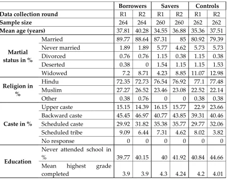
Married 89.77 88.64 87.31 85 80.92 79.39 Never married 1.89 1.89 5.77 4.62 5.73 5.73 Divorced 0.76 0.76 1.15 0.38 1.15 0.38 Deserted 0.38 0 1.54 1.15 1.15 1.53 Widowed 7.2 8.71 4.23 8.85 11.07 12.98
Religion in %
Hindu 72.35 72.73 76.54 76.92 77.1 77.48 Muslim 27.27 26.52 23.46 23.08 22.52 22.14 Other 0.38 0.76 0 0 0.38 0.38
Caste in %
Upper caste 15.15 14.39 16.15 15.77 22.9 23.66 Backward caste 45.45 46.97 40.77 43.85 39.31 40.46 Scheduled caste 29.92 31.82 35.38 35.77 29.77 32.06 Scheduled tribe 9.09 6.44 7.31 4.62 8.02 3.82
No response 0 0 0 0 0 0
Education
Never attended school in
% 39.77 40.15 40 41.92 40.84 44.66 Mean highest grade
completed 3.9 3.9 4.3 4.24 4.2 4.01
Source: Author’s own calculations.
22 capital. SEWA Bank provides loans for a range of purpose, e.g. business, housing improvements/repairs, repayment of other debts and consumption but without a particular focus on micro-enterprise development.
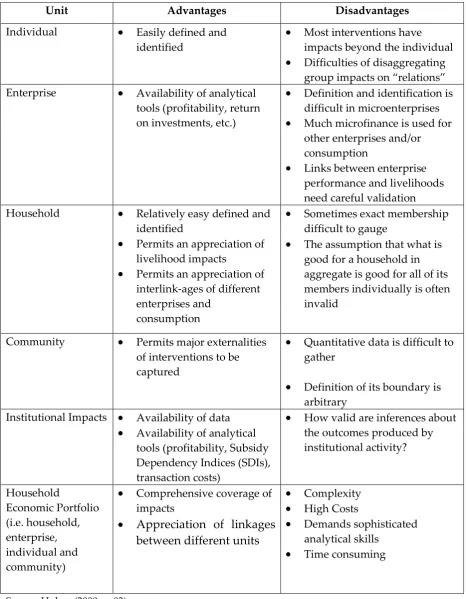
Fungibility of money is a central problem in the context of microfinance impact evaluations and notoriously difficult to control for (Hulme, 2000). Money is considered to be fungible within the household, i.e. once a loan has been taken out by the borrower, it is difficult to track in which way the loan has actually been used (Ledgerwood, 1999). Based on the findings of the USAID study, it appears that measuring impact separately at the enterprise and individual level does not lead to particularly satisfactory results, and this is likely at least partly to be because of fungibility.
23
Table 3: Units or levels of evaluation and their advantages and disadvantages
Unit Advantages Disadvantages
Individual • Easily defined and
identified
• Most interventions have
impacts beyond the individual
• Difficulties of disaggregating
group impacts on “relations”
Enterprise • Availability of analytical
tools (profitability, return on investments, etc.)
• Definition and identification is
difficult in microenterprises
• Much microfinance is used for
other enterprises and/or consumption
• Links between enterprise
performance and livelihoods need careful validation
Household • Relatively easy defined and
identified
• Permits an appreciation of
livelihood impacts
• Permits an appreciation of
interlink-ages of different enterprises and
consumption
• Sometimes exact membership
difficult to gauge
• The assumption that what is
good for a household in aggregate is good for all of its members individually is often invalid
Community • Permits major externalities
of interventions to be captured
• Quantitative data is difficult to
gather
• Definition of its boundary is
arbitrary
Institutional Impacts • Availability of data
• Availability of analytical
tools (profitability, Subsidy Dependency Indices (SDIs), transaction costs)
• How valid are inferences about
the outcomes produced by institutional activity? Household Economic Portfolio (i.e. household, enterprise, individual and community)
• Comprehensive coverage of
impacts
• Complexity
• High Costs
• Demands sophisticated
analytical skills
• Time consuming
• Appreciation of linkages between different units
24 As mentioned earlier, the aim of this study is to re-visit the evidence of microfinance impact evaluations; hence the USAID panel data set has been subjected to more advanced econometric techniques, i.e. PSM to account for selection bias (see claims by Dehejia and Wahba, 1999 and 2002). In addition, a new cross-section data set (henceforth Round 3) was produced, with the aim of exploring the potential of indicators of social capital to illuminate the role of the unobservables and to compare the USAID panel with Round 3 to get a clearer picture on short-term versus long-term impacts of microfinance. However, the Round 3 data have shortcomings. A further round of the panel could not be collected as neither the original panel sample SEWA Bank members not the controls could be identified. The sample size of 220 households is rather small because of budget and time constraints. Hence, the Round 3 data comparability to the USAID data is limited. Another point is that PSM requires rich and high quality data sets (Smith and Todd, 2005), but there are many missing data in Round 3, in particular in the social capital and the housing improvements section, which limits its explanatory power; hence Round 3 quantitative data are not further discussed in this paper.5 To conclude, it appears that
low-cost and small surveys such as the Round 3 survey do not necessarily add value and do not provide accurate impact estimates.
6
Estimation strategy
This study replicates the USAID analysis and subjects these data to PSM to control for selection bias in the hope of providing more reliable impact estimates. PSM matches participants to non-participants on the basis of observable characteristics and compares outcomes between the treatment sample and the sample of matches (Caliendo and Kopeinig, 2005 and 2008; Rosenbaum and Silber, 2001). The underlying assumption is that there is no selection bias due to unobservable characteristics, though, whether this assumption holds is questionable; this is examined using sensitivity analysis of the PSM results which can suggest the presence and likely size of the effect of selection on unobservables (Rosenbaum, 2002). We have seen earlier that in the case of microfinance unobservables are very likely to be present.
To begin with, the empirical model is outlined. As mentioned earlier, the USAID study collected data on three sub-samples: borrowers, savers and controls. The
25 objective is to assess the socio-economic impact of microfinance participation. Consider the following empirical specification; i stands for household in ward j:
(1)
𝑦𝑖𝑗 = C𝑖𝑗δ+ X𝑖𝑗α+ 𝑉𝑗β+ ε𝑖𝑗
Where:
𝑦𝑖𝑗 = outcome on which impact is measured
C𝑖𝑗 = level of participation in microfinance, i.e. a membership dummy variable
δ = effect of the microfinance programme, main parameter of interest X𝑖𝑗 = vector of household level characteristics
𝑉𝑗 = vector of ward level characteristics 𝛼,β = unknown parameters
ε𝑖𝑗 = error term representing unmeasured household and ward characteristics that
can influence outcomes
26
Table 4: Logit regression of probability of microfinance participation, without sampling weights6
Independent variables Round 1 Round 2
Age household head -0.040*** -0.002
0.000 0.823
Age respondent 0.019* 0.010
0.057 0.341
Highest grade completed male 0.083*** 0.001
0.003 0.956
Respondent married (yes=1) 0.789*** 0.760***
0.004 0.008
Muslim (yes=1) 0.510** 0.434**
0.013 0.030
Upper Caste (yes=1) -0.666*** -0.682***
0.003 0.001
Household size 0.011 -0.074
0.920 0.422
Nuclear household (yes=1) -0.453** -0.293
0.042 0.174
Non-SEWA savings -0.000 -0.000
0.190 0.695
Constant -0.360 -0.413
0.713 0.679
Number of observations 768 785
Pseudo R-squared 0.059 0.032
Source: Author’s own calculations.
Notes: p-values in italics. *statistically significant at 10%, **statistically significant at 5%, ***statistically significant at 1%. Please also note that the following control variables were included in the logit model: age, age squared, highest grade completed household head, highest grade completed respondent, sex household head (male=1), number of adult male in household, number of household members aged 0-14, subnuclear household (yes=1); all insignificant.
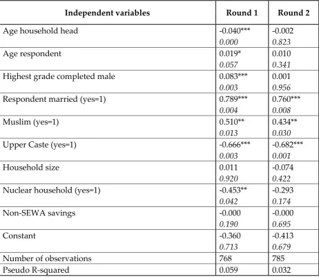
Table 4 presents the logit regression estimating the probability of microfinance participation. The logit model is required to predict the propensity scores so that the matching procedure can be implemented – section 7 outlines this in more depth. The
[image:27.595.67.530.113.513.2]
27 results presented in Table 4 show that the main variables associated with membership that are statistically significant in rounds 1 and 2 are being married, Muslim and upper caste. In addition, age of household head, age of respondent, highest grade completed male and nuclear household are significant in round 1. Few covariates are statistically significant and the values for the pseudo R-squared across both rounds are rather low which indicates that the model has limited explanatory power.7
7
Results
The findings with respect to selected hypotheses are presented in this section. The individual and enterprise level hypotheses of the USAID study led to mixed and rather insignificant results. As argued earlier, measuring impact at these levels is unsatisfactory, and the household level is the most promising way to obtain meaningful impact estimates. Hence, this section focuses on selected household level results only, i.e. on income, housing expenditure and children’s education.8
Firstly, the selected household level results of the USAID study are replicated. Replication is an important step in validating results (Hamermesh, 2007). Hence, the USAID data9 were subjected to ANOVA and ANCOVA. My replication closely
reproduced the USAID study results and is thus not discussed further.
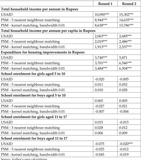
Next, PSM is employed on the USAID data to gauge whether more advanced econometric techniques than ANOVA and ANCOVA, which claim to account for selection bias (Chen and Snodgrass, 2001), would produce different results. The original household level results of the USAID study are compared with the results obtained when PSM was applied using 5-nearest neighbour matching and kernel matching with a bandwidth of 0.01 (Table 5). Participants, i.e. borrowers and savers together, versus controls are presented first. Further sub-group comparisons are presented later in this paper.
7 I experimented with the logit model and tried various other control variables with the objective to enhance the explanatory power of the model but to no avail. The low explanatory power of the model has implications for the reliability of my PSM results; this is further investigated in section 7.3 where sensitivity analysis is introduced.
8 The detailed and re-analysed results of all household level as well as individual and enterprise level hypotheses of the USAID study can be obtained from the author upon request.
28 Before discussing the results presented in Table 5 and Table 8 in more detail, a few remarks with regard to the implementation of PSM are required. The basic idea of matching is to compare a participant with one or more non-participants who are similar in terms of a set of observed covariates X (Caliendo and Kopeinig, 2005 and 2008). This requires predicting propensity scores for each individual, i.e. participants as well as non-participants using a logit or a probit model. I used the logit model presented in Table 4 to predict those propensity scores. Then, before implementing the actual matching process, I examined whether the propensity scores I had obtained for participants and non-participants fulfil the common support assumption. Caliendo and Hujer (2005) express the common support assumption as follows:
(2) 0 < Pr (𝐷= 1 | 𝑋) < 1
This assumption indicates whether treatment and control groups provide equal support of X (Caliendo, 2006). This can be investigated graphically. Figure 1 presents the distribution of the propensity score for participants as well as non-participants; it shows that each participant with a certain propensity score has a corresponding participant. In other words, if the propensity scores for participants and non-participants overlap reasonably well, then the common support assumption is satisfied and it is recommended comparing those two groups. Next, the differences in the outcome variables for participants and their matched non-participants are calculated (Morgan and Harding, 2006) as presented in Table 5 and Table 8. Furthermore, I used t-tests10
Table 5
before and after matching for all results presented in and Table 8 to examine the differences of the mean values for each covariate X across treatment and control groups. In addition, those t-tests calculated a ‘bias’ defined as the mean value of the treatment group and the (matched/unmatched) control group divided by the square root of the average sample variance in the treatment group and the (matched/unmatched) control group. The t-tests I employed indicate that the differences between treatment and control groups as well as the ‘bias’ were reduced considerably in most cases, hence the matching process was successful in generating a control group that was reasonably similar to the treatment group. Therefore, the use of PSM is justified in this case. As a consequence, I conclude that the balancing properties of the propensity scores were satisfied in all cases.
10
29
Figure 1: Distribution of propensity scores for participants and non-participants
Source: Author’s own calculations.
.2 .4 .6 .8 1
Propensity Score
30
Table 5: PSM impact estimates of selected household level results – microfinance participants versus controls; without sampling weights11
Round 1 Round 2
Total household income per annum in Rupees
USAID 10,090*** 15,302***
PSM - 5 nearest neighbour matching 8,944*** 14,635*** PSM - kernel matching, bandwidth 0.01 8,638*** 13,786***
Total household income per annum per capita in Rupees
USAID 2,063*** 2,685***
PSM - 5 nearest neighbour matching 2,019*** 2,486*** PSM - kernel matching, bandwidth 0.01 1,913*** 2,537***
Expenditure for housing improvements in Rupees
USAID 3,748*** 5,871
PSM - 5 nearest neighbour matching 3,701*** 6,546*** PSM - kernel matching, bandwidth 0.01 3,484*** 6,504***
School enrolment for girls aged 5 to 10
USAID -0.020 -0.005
PSM - 5 nearest neighbour matching 0.011 0.052 PSM - kernel matching, bandwidth 0.01 0.010 0.028
School enrolment for boys aged 5 to 10
USAID 0.065 0.005
PSM - 5 nearest neighbour matching -0.027 0.021 PSM - kernel matching, bandwidth 0.01 -0.007 -0.004
School enrolment for girls aged 11 to 17
USAID 0.015 -0.015
PSM - 5 nearest neighbour matching 0.028 0.012 PSM - kernel matching, bandwidth 0.01 0.006 0.009
School enrolment for boys aged 11 to 17
USAID -0.075 -0.020***
PSM - 5 nearest neighbour matching -0.025 -0.012 PSM - kernel matching, bandwidth 0.01 -0.045 -0.019
Source: Author’s own calculations.
Notes: *statistically significant at 10%, **statistically significant at 5%, ***statistically significant at 1%. The results in this table refer to the differences in the mean values between matched samples; they were obtained using the STATA command psmatch2. I also ran the STATA command pscore with the
[image:31.595.68.530.111.634.2]
31
objective to cross-check the psmatch2 results across the various matching algorithms. The results I obtained from the different STATA routines displayed minor differences in terms of the size of coefficient and the level of significance. Morgan and Winship (2007) argue that matching results can vary depending on the matching algorithm and PSM routine applied. Results are bootstrapped.
7.1
Income
12The results for income per annum13, income per annum per capita14
12 All income figures throughout this study have been deflated to January 1998 prices by using a deflator of 1.156 – as mentioned in the USAID study. This was the value of the Consumer Price Index (CPI-IW) for Ahmedabad in January 2000, expressed on a base of January 1998.
and expenditure for housing improvements are positive and statistically significant across rounds 1 and 2. Those results reflect the differences between participants and non-participants. For example, according to the USAID round 1 result; income per annum was higher by 10,090 Rupees for microfinance participants than for non-participants whereas the PSM results applying 5-nearest neighbour matching show that income per annum increased by 8,944 Rupees for participants. Similarly, the PSM results applying kernel matching with a bandwidth of 0.01 display an increase in income per annum by 8,638 Rupees for microfinance participants. It can be seen that the degree of impact depends on the econometric technique applied but even when the same technique is applied, i.e. PSM, the impact estimates still vary - though not substantively so - because of the different matching algorithms applied. For example, kernel matching estimates with a bandwidth of 0.01 for income per annum and for income per annum per capita are lower than the respective 5-nearest neighbour matching estimates for rounds 1 and 2. Also, when the bandwidth increases in the case of kernel matching, the impact estimate tends to increase as well. However,
13 Income per annum is confounded with household size and hence an unreliable measure of outcome. However, since USAID assesses the impact on income per annum and since I am comparing their results with mine, I will continue to report income per annum results throughout the paper. Nonetheless, the reader should treat those results with caution.
32 these observations are not common to all outcome variables or rounds as Table 5 clearly demonstrates.
Overall, in the case of income per annum, income per capita and expenditure for housing improvements across round 1 and 2, the general trend and the statistical significance are similar across USAID and PSM results. In other words, the results obtained by applying PSM appear to support the original findings of USAID with the exception that the USAID results for expenditure for housing improvements in round 2 were not statistically significant while the PSM results are statistically significant.
7.2
School enrolment
The PSM results for school enrolment for girls aged 5 to 10 across rounds 1 and 2 display a positive trend, i.e. participants do better than non-participants, but none of the results are statistically significant. The respective USAID results are negative but also insignificant. The results for school enrolment for girls aged 11 to 17 across round 1 and 2 are equally meaningless, USAID argues that there is an increase in school enrolment in round 1 but the impact estimate is suddenly negative in round 2. The PSM results are all positive but insignificant.
The picture does not change dramatically when looking at school enrolment figures for boys aged 5 to 10 and 11 to 17. According to the PSM results across all three rounds, microfinance has negative impacts on the school enrolment of boys aged 5 to 10 with the exception of one value in round 2 obtained by applying 5-nearest neighbour matching which implies a negligible positive impact. The USAID results, on the other hand, indicate a positive impact but none of the results are statistically significant. Chen and Snodgrass (2001) argue that most boys in the age group 5 to 10 are in fact already enrolled in school irrespective of microfinance participation. All enrolment figures for boys aged 11 to 17 are negative across USAID and PSM results for round 1 and 2 with one figure being statistically significant. Hence, it can be concluded that microfinance participation does not seem to have any significant impact on children’s education.
33
7.3
Sensitivity analysis
The impact evaluation of SEWA Bank needs to answer the question whether the apparent effect of membership compared to the control group is due to the saving and borrowing enabled by membership of SEWA Bank or some unobserved characteristic of members compared to the control group, such as entrepreneurial abilities, access to social networks, etc. PSM allows control for observable characteristics included in the propensity score on which members and controls are matched, but it cannot control for unobservables (Caliendo and Kopeinig, 2005 and 2008; Rosenbaum and Silber, 2001). Rosenbaum (2002) developed the “conceptual advance” (ibid, p. 106) of Cornfield et al (1959) that the robustness of the estimate of the difference in outcome between treatment and control groups (the impact estimate) could be assessed by asking what magnitude of selection on unobservables (hidden bias) one would need in order to explain away the observed impact, thus: “[I]f the association [Author’s note: between treatment and outcome] is strong, the hidden bias needed to explain it is large” (Rosenbaum, 2002, p. 106). In the context of death from lung cancer for smokers and non-smokers Cornfield et al (1959) suggested that if the ratio of the likelihood of death from lung cancer for smokers to the likelihood of death from lung cancer for non-smokers was high then a similar high ratio for the unobserved characteristic(s) would be required to make this unobserved characteristic the true cause of the higher prevalence of death from lung cancer by smokers.
Rosenbaum (2010) explains that “a sensitivity analysis in an observational study asks how the conclusions of the study might change if people who looked comparable were actually somewhat different…” (p. 367). In other words, the objective of sensitivity analysis is to explore whether the matching estimates are robust to selection on unobservables (Rosenbaum, 2002). Ichino, Mealli and Nannicini (2006) argue that “sensitivity analysis should always accompany the presentation of matching estimates” (p. 19).
Rosenbaum (2002) invites us to imagine a number Γ (gamma) (≥ 1) which captures the required degree of association, of an unobserved characteristic with the treatment, for it (the unobserved characteristic) to explain the observed impact. Γ is the ratio of the odds15 that the treated have this unobserved characteristic to the odds
that the controls have this characteristic.16
15Odds, which are widely used in assessing probabilistic outcomes, are derived from probabilities (0 ≤
𝜋𝑖≤ 1) by the following formula: 𝜋𝑖⁄(1− 𝜋𝑖).
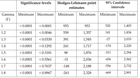
34 This approach can be implemented using the rbounds procedure in STATA (Becker and Caliendo, 2007); this procedure uses the data to calculate the confidence intervals (for a given level of confidence – e.g. 95%) of the outcome variable for different values of Γ. A value of Γ that produces a confidence interval that encompasses zero is one that would make the estimated impact not statistically significant at the relevant level of confidence. If Γ is rela tively sma ll (sa y < 2 ) then one ma y a ssert tha t the likelihood of such an unobserved characteristic is relatively high, and therefore that the estimated impact is rather sensitive to the existence of unobservables (DiPrete and Gangl, 2004). If there is other evidence that there may be unobservables, such as my qualitative observations of the SEWA Bank selection processes, we cannot be confident that the estimated impact is not due to unobservables.
We can illustrate this approach by calculating Γ at which the estimated impact of SEWA Bank membership on household income per capita for round 1 is no longer statistically significant. Table 5 shows that the 5-nearest neighbour matching estimate for total household income per annum per capita in round 1 is 2,019 Rupees which is significant at 1%. This suggests that households participating in microfinance earn significantly more income per annum per capita than control households; however, this may not be due to membership per se but unobserved characteristics that account for membership (and or its impact). Sensitivity analysis explores the robustness of this impact estimate and demonstrates how it changes in the presence of selection on unobservables. The STATA procedure rbounds reports the estimates17
Table 6
and their 95% (or other) confidence intervals for matched pairs of SEWA Bank members and controls (see ).
When Γ = 1 there is no selection on unobservables. If Γ increases to 1.2, then matched individuals differ in their odds of exposure to microfinance by a factor of 1.2 due to selection on unobservables. Table 6 shows that when Γ = 1.2 the statistical significance level ranges from < 0.0001 to < 0.0046. This implies that in this case selection on unobservables is not likely to explain the observed association between exposure to microfinance and higher income levels. However, when Γ = 1.3 or more, a relatively small difference in the odds of exposure implying that it is quite likely that such an unobserved confounding variable exists, the 95% confidence interval of
odds of being selected). Γ =2 means that individual j is twice as likely to be selected into SEWA Bank as individual k. This might be considered not unlikely based on my observations of the selection process operated by SEWA Saathi, and by my understanding of the requirements of households to be able to save, and for other to qualify for borrowing.
35 the point estimates encompasses zero. Consequently, we can argue that the observed impact of SEWA Bank membership on household income per capita is not significantly different from zero, and the association between microfinance exposure and higher income levels may well be due to unobservables.
Table 6: Sensitivity analysis for household income per annum per capita in Rupees for microfinance participants for round 1: magnitude of selection on unobservables, range of significance levels, Hodges-Lehmann point estimates and confidence intervals
Significance levels Hodges-Lehmann point estimates
95% Confidence intervals
Gamma
(Γ) Minimum Maximum Minimum Maximum Minimum Maximum
1 < 0.0001 < 0.0001 953 953 520 1,403
1.2 < 0.0001 < 0.0046 559 1,357 141 1,834
1.3 < 0.0001 < 0.0330 391 1,545 -27 2,033
1.4 < 0.0001 < 0.1292 241 1,717 -174 2,220
1.5 < 0.0001 < 0.3181 98 1,876 -311 2,394
1.6 < 0.0001 < 0.5561 -31 2,036 -436 2,562
1.7 < 0.0001 < 0.7637 -148 2,188 -556 2,732
1.8 < 0.0001 < 0.8967 -261 2,328 -669 2,891
Source: Author’s own calculations. Notes: see footnote 17.
Sensitivity analysis was conducted on all the outcome variables presented in Table 5; testing the sensitivity of all impact estimates on the household, enterprise and individual level across rounds 1 and 2. The evidence provided by those tests are in agreement with the description above, namely that the impact estimates presented in Table 5 are sensitive to selection on unobservables and should be treated with caution.18
18 The detailed results from those sensitivity tests are not presented here but the relevant STATA do-files can be made available upon request.
[image:36.595.67.538.238.502.2]36 the specific effect on the odds ratio of treatment and that it has a strong effect on the outcome variable (DiPrete and Gangl, 2004, p. 291). Nevertheless, PSM and related tests allow the quantification of selection on unobservables which is helpful. These results lead me to concur with Ichino, Mealli and Nannicini (2006), namely that sensitivity testing should always complement the presentation of matching estimates. In this case caution in concluding that SEWA Bank membership has a causal effect on per capita income is warranted.
7.4
Panel analysis
The panel data analysis with or without PSM reveals nothing new and broadly confirms the results obtained from the cross-section analysis. As illustrated in Table 7, PSM using nearest neighbour matching on round 1 data caused some households which did not match on observable characteristics to be dropped, and only matched households were merged with round 2 data. Using the treatment and matched households a regression-adjusted differences-in-differences (DID) model was run on all outcome variables as set out by the following equation which is a fixed effects linear regression model; i stands for household in ward j at period t:
(3) 𝑦𝑖𝑗𝑡 =𝛼𝑖 +𝛿𝑡+𝛽C𝑖𝑡+ θX𝑖𝑡+ 𝑉𝑗+ ε𝑖𝑗𝑡
Where:
𝑦𝑖𝑗𝑡 = outcome on which impact is measured at period t
C𝑖𝑡 = level of participation in microfinance, i.e. a membership dummy variable, in period t
X𝑖𝑡 = vector of household level characteristics in period t
𝑉𝑗 = vector of ward level characteristics
𝛼𝑖 = fixed effects unique to household i
𝛿𝑡 = period effect common to all households in period t β,θ = unknown parameters
ε𝑖𝑗𝑡 = error term representing unmeasured household and ward characteristics at
period t
37
Table 7: PSM and DID results - impact of microfinance participation; without sampling weights19
Household level hypotheses
Total household income per annum in Rupees 11,287*** Total household income per annum per capita in Rupees 2,181***
Inverse Simpson index 0.121
Expenditure for housing improvements in Rupees 5,628*** Expenditure on household assets in Rupees 734** School enrolment for girls aged 5 to 10 -0.019 School enrolment for boys aged 5 to 10 0.019 School enrolment for girls aged 11 to 17 0.025 School enrolment for boys aged 11 to 17 -0.011 Food expenditure per day per capita in Rupees 0.93
Enterprise level hypotheses
Informal sector income of whole household - per month in Rupees 3,091** Informal sector income of respondent only - per month in Rupees 1,876** Microenterprise revenues of all enterprises in household - per month in
Rupees 3,050**
Microenterprise revenues of microenterprises for which respondent is
primarily responsible - per month in Rupees 1,559** Current value of fixed assets of all microenterprises in household in
Rupees 211
Current value of fixed assets of microenterprises for which respondent
is primarily responsible in Rupees 482 Hours worked in previous week in all microenterprises in household 13.78*** Days worked in previous month in all microenterprises in household 10.17*** Main types of suppliers - inferior20 suppliers? Yes=1, No=0 0.060*
Main types of customers - inferior21 customers? Yes=1, No=0 0.083** Individual level hypotheses
Respect by other household members? Yes=1, No=0 0.015 Prepared to deal with future? Yes=1, No=0 0.019
Source: Author’s own calculations.
Notes: *statistically significant at 10%, **statistically significant at 5%, ***statistically significant at 1%. The STATA procedure xtreg was applied to implement DID.
19 As discussed in footnote 6 and 11.
20 Individuals/households and retailers are inferior sources of supply as defined by Chen and Snodgrass (2001).
38 These findings are broadly in agreement with the results that USAID presented. However, caution is required when interpreting the panel data findings. One would have expected some differences between the cross-section and panel data results since panel analysis should account for the unobservables but, this appears not to have been the case in this study. However, one could argue that the USAID dataset is not a real panel with a ‘true’ baseline because round 1 respondents were already microfinance clients when the baseline dataset was collected. The same clients and control households were then re-surveyed two years later. Strictly speaking, the baseline should have collected data on households that were not participating in microfinance at the time of the baseline data collection but became microfinance clients between survey rounds. This would have allowed a before and after comparison which would have been better suited to the analysis because it would have been possible to compare the treatment and control households in terms of all observables including outcomes; this would have allowed one to assess whether these two samples were broadly similar in these terms, although it would still not be possible to control for unobservables which affect response to the treatment.
7.5
Summary
Most of the PSM results confirm the findings of the USAID study if one ignores unobservables. What does this outcome mean for the issue of selection bias and the utility of PSM? Chen and Snodgrass (2001) argue that ANCOVA using a suitable control group accounts for selection bias to a certain degree. Based on the PSM results presented in Table 5, the first impression is that this assessment is indeed accurate. However, doubts remain as there are strong qualitative and theoretical reasons to think that unobservables have not been fully controlled for. This notion is confirmed by the sensitivity analysis which shows that the matching estimates are quite sensitive to selection on unobservables.
39
7.6
Sub-group comparisons
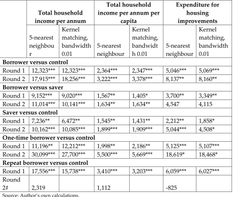
Having reached these preliminary conclusions with regard to membership of SEWA Bank, whether as saver or (saver and) borrower, sub-group comparisons were conducted to understand the impact of savings compared to saving and borrowing. As argued in section 3 and 4, Ghate (2007), as well as many microfinance practitioners, believe that the poor need savings more than credit. The following comparisons were investigated: borrowers versus controls, savers versus controls, borrowers versus savers, one-time borrowers versus savers, repeat borrowers versus savers, one-time borrowers versus controls and repeat borrowers versus controls. Again, only the key findings are presented. The results of the comparisons of the various borrower groups with savers are similar to the various borrower group comparisons with controls in terms of absolute numbers and level of significance, hence only the latter comparisons are discussed.22
40
Table 8: Selected household level PSM results – sub-group comparisons; without sampling weights23
Total household income per annum
Total household income per annum per
capita Expenditure for housing improvements 5-nearest neighbou r Kernel matching, bandwidth 0.01 5-nearest neighbour Kernel matching, bandwidt h 0.01 5-nearest neighbour Kernel matching, bandwidth 0.01
Borrower versus control
Round 1 12,323*** 12,323*** 2,364*** 2,347*** 5,046*** 5,069*** Round 2 17,915*** 18,256*** 3,222*** 3,378*** 8,137** 8,160**
Borrower versus saver
Round 1 9,152*** 9,020*** 1,567** 1,405* 3,700** 3,349** Round 2 11,014*** 10,141*** 1,634** 1,634** 4,547 4,115
Saver versus control
Round 1 7,236** 6,472** 1,545** 1,431** 2,212** 1,858* Round 2 10,162*** 10,085*** 1,899*** 1,909*** 5,044*** 4,508*
One-time borrower versus control
Round 1 11,196** 12,212*** 1,998** 2,186** 5,125*** 5,107*** Round 2 30,099*** 27,700*** 5,500*** 5,669*** 18,619* 18,468*
Repeat borrower versus control
Round 1 17,556*** 15,738*** 3,410*** 3,203*** 6,059*** 6,027*** Round
2# 2,319 1,112 -825
Source: Author’s own calculations.
Notes: *statistically significant at 10%, **statistically significant at 5%, ***statistically significant at 1%. All figures in Indian Rupees. The results in this table refer to the differences in the mean values between matched samples; they were obtained using the STATA command psmatch2. I also ran the STATA command pscore with the objective to cross-check the psmatch2 results across the various matching algorithms. The results I obtained from the different STATA routines displayed minor differences in terms of the size of coefficient and the level of significance. Morgan and Winship (2007) argue that matching results can vary depending on the matching algorithm and PSM routine applied. # No values for kernel matching in round 2, the sample was too small with propensity scores outside the common support region, no adequate matches were found. Results are bootstrapped.
The discussion of sub-group comparisons focuses on selected household level hypotheses, namely income per annum, income per annum per capita24
23 As discussed in footnotes
and
[image:41.595.66.534.113.505.2]