Droplet formation in microfluidic cross-junctions

Droplet formation in microfluidic cross-junctions

Haihu Liua)and Yonghao Zhangb)

Department of Mechanical Engineering, University of Strathclyde, Glasgow G1 1XJ, United Kingdom

(Received 11 January 2011; accepted 29 June 2011; published online 4 August 2011)

Using a lattice Boltzmann multiphase model, three-dimensional numerical simulations have been performed to understand droplet formation in microfluidic cross-junctions at low capillary numbers. Flow regimes, consequence of interaction between two immiscible fluids, are found to be dependent on the capillary number and flow rates of the continuous and dispersed phases. A regime map is created to describe the transition from droplets formation at a cross-junction (DCJ), downstream of cross-junction to stable parallel flows. The influence of flow rate ratio, capillary number, and channel geometry is then systematically studied in the squeezing-pressure-dominated DCJ regime. The plug length is found to exhibit a linear dependence on the flow rate ratio and obey power-law behavior on the capillary number. The channel geometry plays an important role in droplet breakup process. A scaling model is proposed to predict the plug length in the DCJ regime with the fitting constants depending on the geometrical parameters. VC _{2011 American}

Institute of Physics. [doi:10.1063/1.3615643]

I. INTRODUCTION

Rapid development of microfabrication technologies has facilitated a broad range of microfluidic applications espe-cially in life sciences. Microdroplet technology has recently emerged as a promising flexible platform for microfluidic functions.1–4 The miniaturization of entire process enables the rapid analysis of very small quantities of samples in a portable, automated, and inexpensive format.3 Recently, microdroplet technology has been used as microreactors for chemical analysis and protein crystallization,5,6as molds for curing polymeric microspheres.7,8 Furthermore, program-mable fluidic assays for sampling glucose concentration of human physiological fluids9and DNA analysis10 have been individually demonstrated using microdroplet system. As samples=reagents are confined in droplets so that sample dilu-tion caused by Taylor dispersion11can be avoided, and mix-ing performance can be improved.12In addition, it can avoid sample=surface interaction and thus eliminate surface adsorp-tion and cross sample contaminaadsorp-tion.

Many microfluidic devices have been designed to generate uniform droplets, including geometry-dominated devices,13,14 flow-focusing devices,15–19 T-junctions,20–26 and co-flowing devices.27,28 However, the underlying mechanisms of droplet formation in microchannels have not been well understood, which hinders device optimization and operation. The two-phase flow characteristics in microchannels are determined by flow conditions, channel geometry, and fluids properties. Guil-lot and Colin22experimentally observed that, for a given flow rate of the continuous phase, the flow pattern changes from droplets at T-junction to droplets in channel if the flow rate of the dispersed phase increases. This indicates that for a given capillary number Ca¼gcuc=r (gc, uc are the viscosity and

velocity of the continuous phase; r is the interfacial tension

coefficient), when the flow rate ratio Q¼Qd=Qc(Qdand Qc

are volume flow rate of the dispersed and continuous phases, respectively) increases, a flow regime change occurs. With a further increase inQ, the flow regime changes to parallel flow. Tanet al.18also found that the two-phase flow patterns depend on the flow rates of the continuous phase and the dispersed phase for the plug formation in a microfluidic cross-junction, which is similar to the observation of Guillot and Colin.22

The channel geometry has been found to play an impor-tant role in the droplet formation process. For example, Garstecki et al.23 identified a squeezing mechanism due to confined microchannel geometry in droplet formation pro-cess, which does not exist in an unbounded flow condition. By studying the underlying mechanisms that control the drop-let breakup, some scaling laws have been established to pre-dict the size of droplets produced in microfluidic devices.29,30 However, the currently available experimental data are still sporadic. Various materials are used to fabricate the micro-channels with diverse dimensions, and the experiments have been performed at different flow conditions with different flu-ids. Consequently, the information is fragmented, which leads to inconclusive and even incompatible findings. Based on sta-tistical analysis of the broad range of available literature data, Steegmanset al.30have shown that none of the scaling mod-els, which are developed to predict droplet formation in a microfluidic T-junction, is general enough to describe the original data and data from other literature sources. Also, they found that the available literature data could be better represented by a two-step model consisting of a growth phase and a detachment phase.

Meanwhile, experiments at such small scales are still difficult. For example, it is challenging to accurately measure local flow fields, droplet deformation, breakup, and coales-cence. Numerical study can be complementary to experimen-tal investigation. For example, Menech et al.25numerically identified three distinct mechanisms, i.e., squeezing, drip-ping, and jetting in droplet formation in a T-junction. How-ever, much effort is still required to numerically simulate a)

Present address: Department of Civil and Environmental Engineering, Uni-versity of Illinois at Urbana-Champaign, Illinois 61801, USA. Electronic mail: [email protected].

b)

Electronic mail: [email protected].

droplet generation, transportation, and interaction with sur-face. While the front tracking methods are not suitable for droplet breakup and coalescence, the interface capturing methods such as volume-of-fluid and level set methods will experience numerical instability when interfacial tension becomes a dominant factor in microdroplet behavior.31 Recently developed lattice Boltzmann (LB) method has shown great potential for modeling interfacial interactions while incorporating fluid flow as a system feature.32 It is a pseudo-molecular method tracking evolution of the distribu-tion funcdistribu-tion of an assembly of molecules and built upon mi-croscopic models and mesoscopic kinetic equations.33 Its mesoscopic nature can provide many advantages of molecu-lar dynamics, making the LB method especially useful for simulation of droplet dynamics.23,34–37

In this work, a multiphase lattice Boltzmann model is employed to investigate droplet formation in microfluidic cross-junctions. We will first present our simulation results that reveal the influence of capillary number and flow rate ra-tio on the flow regime transira-tion from droplet generara-tion at cross-junction (DCJ), downstream of the cross-junction (DC), to parallel flows (PF). In the DCJ regime, the influences of capillary number, flow rate ratio, and channel geometry will be studied in details. We will compare our simulation with the existing models and experimental data. To our best knowledge, this is for the first time that numerical simulations are performed to identify the flow regimes and investigate the effect of channel geometry on the droplet formation in

micro-fluidic cross-junctions. This study can provide useful infor-mation for understanding microdroplet dynamics and optimal design of multiphase microfluidic devices.

II. NUMERICAL METHOD

In the lattice Boltzmann method, a fluid is modeled as pseudo particles, whose distribution function fi is governed

by the lattice Boltzmann equation, e.g., using the Bhatnagar-Gross-Krook (BGK) collision operator32

fiðxþeidt;tþdtÞ ¼fiðx;tÞ 1

s½fiðx;tÞ f eq

i ðx;tÞ; (1)

wherefi(x,t) is the particle distribution function in theith

ve-locity direction at the positionxand the timet,eiis the lattice

velocity in theith direction,sis the dimensionless relaxation time, and fieq is the equilibrium distribution function as a function of local densityqand velocityu

fieq¼wiq 1þ eiu

c2

s

þðeiuÞ

2

2c4

s

uu

2c2

s

" #

; (2)

wherecsdenotes the speed of sound which is given byc=

ffiffiffi

3

p

withc¼dx=dtbeing the lattice speed anddxbeing the lattice

length.

For the three-dimensional 19-velocity (D3Q19) model, the lattice velocityeiand the weight coefficientswiare given as

ei¼

ð0;0;0Þ; i¼0;

ð61;0;0Þc;ð0;61;0Þc;ð0;0;61Þc; i¼1;2;…;6; ð61;6;0Þc;ð61;0;61Þc;ð0;61;61Þc; i¼7;8;…;18; 8

> < >

: (3)

wi¼

1=3; i¼0;

1=18; i¼1;2;…;6;

1=36; i¼7;8;…;18: 8

<

: (4)

The macroscopic properties including the local density and momentum are related to the particle distribution func-tionfiby

q¼X

i fi¼

X

i

f_ieq; qu¼X

i fiei¼

X

i

f_ieqei: (5)

Using the Chapman-Enskog expansion for the D3Q19 model, Eq.(1)can lead to the Navier-Stokes equations in the long-wavelength and low-frequency limit38

@tqþ r ðquÞ ¼0; (6)

@tðquÞ þ r ðquuÞ ¼ rpþ r ðqruÞ; (7)

where the pressure and the kinematic viscosity are given as p¼qc2

s and¼ðs1=2Þc

2

sdt.

Currently, the most applied LB multiphase methods are the color-fluid model,39the pseudo-potential model,40and the free-energy model.41,42In the color-fluid model, the procedure of redistribution of the colored density at each node to separate

different phases requires time-consuming calculation of local maxima, and the perturbation step with the redistribution of colored distribution functions causes an anisotropic interfacial tension that induces high spurious velocities near interface.38 The pseudo-potential model introduces the nearest-neighboring interaction between fluid particles to describe the intermolecu-lar potential, and the phase separation occurs with a properly chosen potential function. Although significant advances have recently been made,43–45 further improvements are necessary for the pseudo-potential model to minimize spurious velocities at interface and control numerical instability for the flows with low capillary number and viscosity ratio. The free-energy model suffers from the lack of Galilean invariance,32although the local conservation of mass and momentum is satisfied. Based on the original color-fluid model of Gunstensen et al., the recent improvements have been made by Lishchuket al.46 and Latva-Kokko and Rothman,47which facilitate simulational access to flow regimes of low Reynolds and capillary numbers. In this study, we will use the improved color-fluid model, because the Reynolds number and the capillary number are typically small in microfluidic droplet formation.

In the original color-fluid model of Gunstensenet al.,39 “Red” and “Blue” particle distribution functions fR

were introduced to represent two different fluids. The total particle distribution function is defined asfi¼fiRþf

B i . Each of the colored phases undergoes the collision and streaming operations

fikðxþei;tþ1Þ ¼fikðx;tÞ fk

iðx;tÞ f k;eq i ðx;tÞ

sk þX

k i; (8)

wherek¼Ror B denotes the color (“Red” or “Blue”). The viscosity of each fluid can be selected by choosing the desiredsk, i.e.,k¼cs2ðsk1=2Þ. Conservation of mass for each phase and total momentum conservation require

qk¼

X

i fik¼

X

i

fik;eq; (9)

qu¼X

i

X

k fikei¼

X

i

X

k

fik;eqei: (10)

The additional collision operatorXk

i (perturbation step) con-tributes to the mixed interfacial regions and generates an interfacial tension

Xk

i ¼AkjGjcos 2ðhihfÞ; (11)

whereAkis a free parameter controlling the interfacial

ten-sion,hiis the polar angle of the lattice vectorei, andhfis the

polar angle of the local color gradientG, which is defined as

Gðx;tÞ ¼X

i

wiei½qRðxþei;tÞ qBðxþei;tÞ: (12)

To promote phase segregation and maintain interface, the so-called recoloring step is applied, which enables to keep the interface sharp, and at the same time prevents the two fluids from mixing with each other. The colors are demixed by maximizing the work done against the color flux q(x, t), which is defined by

qðx;tÞ ¼X

i

wiei½fiRðx;tÞ f B

i ðx;tÞ: (13)

The perturbation step can introduce anisotropy and high spurious velocities at the interface. Additionally, when applied to study creeping flows, the recoloring step can pro-duce lattice pinning,47a phenomenon that the interface can be pinned or attached to the simulation lattice rendering an effective loss of Galilean invariance. It was also demon-strated that there is an increasing tendency for lattice pinning as both of the capillary and Reynolds numbers decrease.48

Lishchuk et al.46used the concept of a continuum sur-face force (CSF)49 to model the interfacial tension. In their algorithm, the perturbation step in the original Gunstensen model was replaced by a direct forcing term at the mixed region. In order to satisfy the stress boundary condition and the continuity of velocity, a local pressure gradient is forced throughout the interface as an additional body forceF(x,t), which is incorporated into the LB equation by the forcing term/i(x,t) at the collision step. It has been reported that

this algorithm can greatly reduce the spurious currents and improve the isotropy of the interface. The body force is defined to act normal to the interface with a magnitude pro-portional to the gradient ofqN, which is given by

Fðx;tÞ ¼ 1

2rjrq

N_{; (14)}

wherer is an interfacial tension parameter,qNis the phase field defined as

qNðx;tÞ ¼qRðx;tÞ qBðx;tÞ

qRðx;tÞ þqBðx;tÞ

; 1qN1; (15)

andjis the local interface curvature, which is calculated by

j¼ rsn; (16)

where rs¼ðInnÞ r is the interface gradient opera-tor, andIis the second-order identity tensor. The unit normal vectornis defined as a function of phase field

n¼ rq

N

jrqN_j: (17)

Based on the body force term given by Eq. (14), the forcing term /i can realize the interfacial tension effect,

which is given as46

/iðx;tÞ ¼ 1 c2

s

wieiFðx;tÞdt: (18)

The calculation of partial derivatives is required to evaluate the interface curvature and the normal vector. To minimize the discretization error, these derivatives are calculated using 19-point finite difference stencils

@wðxÞ @xa ¼

1 c2

s

X

i

wiwðxþeiÞeia: (19)

In addition, the original recoloring step is modified by an anti-diffusion scheme proposed by Latva-Kokko and Rothman,47 which can solve the lattice pinning problem and creates a sym-metric distribution of particles around the interface so that the spurious velocities can be further reduced. Following their method, the post-collision, postsegregation (recolored) particle distribution functions for the red and blue fluids are calculated by

fiR¼ qR qRþqB

fiþb qRqB qRþqB

wicosujeij; (20)

fiB¼ qB qRþqB

fib qRqB qRþqB

wicosujeij; (21)

where fi denotes the post-collision, presegregation value of

the total particle distribution function along the ith lattice direction;bis the segregation parameter and is fixed at 0.7 to maintain a narrow interface thickness and reduce spurious velocities;50and also, we will show that this choice is neces-sary to reproduce correct dynamical behavior of droplets;u is the angle between the color gradient rqN _{and the lattice} vectorei, which is defined by

cosu¼ ei rq

N

jeijjrqNj

: (22)

III. RESULTS AND DISCUSSION

droplet is placed between two parallel plates that are moving in the opposite directions to obtain a linear shear in the Stokes flow regime (i.e., small Reynolds number). Droplet deformation is studied as a function of the shear rate via the capillary number. The definitions of the Reynolds number and capillary number are given as

Re¼cR

2_q

g ; Ca¼ cRg

r ; (23)

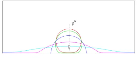
wherec¼2U=His the shear rate with Ubeing the velocity of the moving plate, andHbeing the channel height;Ris the initial radius of the droplet. For this case, we assume that both fluids have the same density and viscosity. The simula-tions are run atRe¼0.1 for a droplet with the radius of 10 lattice cells in a system of 1005050 lattice cells. At the steady state, the droplet is assumed to be ellipsoidal, which is usually characterized by the deformation parameter Df, defined as

Df ¼ab

aþb; (24)

whereaandbare the lengths of the major and minor axis of the deformed droplet, respectively. For a droplet in the Stokes regime with a lowCa,Dffollows the Taylor relation as51

Df ¼ ð35=32ÞCa: (25)

A series of numerical simulations are performed with b¼ f0.5, 0.7, 1g and Ca varying from 0.05 to 0.3. Fig. 1 shows the time evolution of Taylor deformation parameter for differentCaandb. We can observe that the droplet can-not evolve to a steady state forb¼1, while a steady droplet deformation can be reached for bothb¼0.5 and 0.7. How-ever, a smallb(i.e., a large interface thickness) usually pro-duces a large droplet deformation at a fixed Ca, which can

be clearly seen in Fig. 2. Meanwhile, the LB simulations withb¼0.7 are in good agreement with the theoretical Tay-lor relation. Therefore, we will use b¼0.7 in the following simulations in order to reproduce the correct droplet dynamics.

The geometry of cross-junction microchannel is illus-trated in Fig.3. The microchannel consists of a main channel with widthwdand two lateral channels with the same width

wc. The depthhis uniform throughout the channels. The

dis-persed phase water is introduced at the inlet of the main channel, and the continuous phase oil is injected into the lat-eral channels. Halfway bounce-back is used at the solid walls in order to obtain no-slip boundary condition.32We assume that the fluids are pure single-phase at the inlets and outlet, and the constant inlet flow rates and outlet pressure boundary conditions are imposed following Zou and He.52For simplic-ity, we set the densities of both fluids equal, as the

FIG. 1. (Color online) Evolution of the Taylor deformation parameter for

b¼ f0.5, 0.7, 1gatCa¼ f0.05, 0.15, 0.3gandRe¼0.1.

FIG. 2. (Color online) Taylor deformation parameterDfas a function of the capillary number atRe¼0.1. The solid line is the theoretical Taylor relation given by Eq.(25).

buoyancy-driven velocities in a typical oil-water microflui-dic system are negligible.25

The wettability of the microchannel walls can strongly influence droplet formation, it is therefore essential to account for the fluid-surface interactions. We follow the assumption made by Rowlinson and Widom53that the solid wall is a mix-ture of two fluids, thus having a certain value of the phase fieldqN

S. The derivatives of phase field near the wall boundary can therefore be calculated using Eq.(19). Consequently, the interfacial force term in Eq.(14)becomes dependent on the properties of the neighboring solid lattice sites, resulting in a special case of the wetting boundary condition. Fig.4 demon-strates that the assigned value of phase field at the solid wall can be used to modify the static contact angle of the interface at the solid surface. Approaches similar to the one described above were also adopted by Bekri and Adler54for the original model of Gunstensenet al.,39 by van der Graaf et al.24 and Liu and Zhang37in the free-energy models and by Shan and Chen40in the pseudo-potential model through the fluid-solid interaction potential. In addition, in the free-energy models, the interaction between fluids and solid surface can be mod-eled by a surface integral that appears in the boundary condi-tion of the free energy.55,56 Unless otherwise stated, we assumeqN

S ¼ 1 in the following simulations so that the con-tinuous phase completely wets the wall surfaces while the dis-persed phase is non-wetting.

The dynamical response of fluids in a microfluidic cross-junction can be described successfully by six independent dimensionless numbers, which are commonly defined by the geometrical and physical parameters including the inlet widths (wcandwd), the channel depth (h), the interfacial tension (r),

the inlet volumetric flow rates (QcandQd), the viscosities (gc

andgd) of the two fluids and their densities (q), where the

sub-scripts “c” and “d” denote the continuous and dispersed phases, respectively. The capillary number (Ca), which describes rela-tive importance of the viscous force and the interfacial tension, is the most important parameter for droplet formation. Here, it is defined by the average inlet velocityucand the viscositygc

of the continuous phase and the interfacial tensionr

Ca¼ucgc

r ¼

Qcgc 2rwch

: (26)

Although the laminar flow is expected due to the small length scales involved, the Reynolds number (Re) is still the most frequently used dimensionless number to effectively describe microfluidics. It is a measure of the ratio of the iner-tial force and the viscous force

Re¼qucwc

gc

¼ qQc

2gch

: (27)

During the process of droplet formation, the continuous phase and the dispersed phase are continuously injected with different volumetric flow rates. The ratio of flow rates (Q¼Qd=Qc) and the viscosity ratio (k¼gd=gc) are two

im-portant dimensionless numbers to characterize the droplet breakup, which has been confirmed by a wide range of ex-perimental and numerical investigations.18,19,23,25,26,37,57The geometrical parameters,wc,wd, andh, lead to two additional

dimensionless parameters characterizing the geometry. One is the ratio of the channel depth to the inlet width of the con-tinuous phase (C¼h=wc), and the other is the ratio of the

inlet widths of the two phases (K¼wd=wc).

Different types of droplets, namely plug droplets, isolate droplets and satellite droplets, can be generated in the cross-junction microfluidic devices, which strongly depend on the various dimensionless parameters.19In the present study, we focus on the formation of plug droplets for a fixed fluid pair, i.e., the viscosities of both fluids and the interfacial tension are fixed, and examine the roles ofCa,Q,C, andKin droplet formation.

A. The influence of Q and Ca

Before we study the influence of geometrical parame-ters, we focus on a reference cross-junction with wc¼10dx,

wd¼20dx, andh¼10dx, so thatC¼1 andK¼2. We choose

a fixed fluid pair with the interfacial tensionr¼0.06 and the viscosity ratio k¼1=6. The simulations are performed in a 2296111 lattice system and each lattice spacingdx

cor-responds to 10lm. We examine the grid independence with several different flow conditions and find that the mesh refinement will lead to results variations not more than 5%. Four different capillary numbers, i.e., Ca¼0.002, 0.004, 0.006, and 0.008 are used in the simulations, and the corre-sponding Reynolds numbers are 0.1, 0.2, 0.3, and 0.4. For each capillary number, the flow rate ratio is varied over a broad range so that the different flow patterns are observed.

As shown in Fig.5, three typical flow patterns are identi-fied for different flow rate ratio at a fixed capillary number. At the low flow rate ratio Q, the droplets are formed at the cross-junction (DCJ) due to the squeezing mechanism. When we increaseQ, droplets are found to pinch-off at DC, form-ing a thread that becomes unstable after a distance of laminar flow. This distance will increase withQ. As the flow rate ra-tioQincreases to a critical value, the stable PF are observed, where the three incoming streams co-flow in parallel to the downstream without pinching. In addition, the transitions from DCJ to DC and from DC to PF are influenced by the capillary number. As Ca increases, the threshold value of flow rate ratio at which the transition occurs decreases, and the width of the DC regime also decreases. The different flow patterns were first observed experimentally by Guillot and Colin in a microfluidic T-junction,22in which the transi-tion from droplets forming at a T-junctransi-tion to stable parallel flow depends on the flow rate of both phases. Recently, Tan et al.18 also reported the similar observations in a FIG. 4. (Color online) The different contact angles obtained through

adjust-ing the phase fieldqN

S at the solid wall. The values of qNS are taken as

qN

microfluidic cross-junction. In the following simulations, we will focus on the DCJ regime so that our simulations can be compared with the existing experimental work.

Based on the experimental observation of plug forma-tion at microfluidic T-juncforma-tions, Garstecki et al.23 argued that at lowCa, the final length of a plug is determined by two steps. First, the thread of the dispersed phase grows until it blocks the continuous phase liquid. At this critical moment, the “blocking length” of the plug is equal to the channel width, i.e., Lblock¼wc. Afterwards, the increased

pressure in the continuous phase liquid begins to “squeeze” the neck of dispersed thread. Assuming that the neck with a characteristic widthdsqueezes at a rate approximately equal to the average velocity (uc) of the continuous phase. During

this time, the plug continues to elongate at rateud ¼_wQ_cd_hwith an equivalent growth of plug volume at rate Qd. So the

“squeezing length” of the plug is Lsqueeze_ud_cud ¼dQ. Therefore, the final lengthLof the plug can be expressed as

L wc

¼LblockþLsqueeze

wc

¼wcþdQ

wc

¼1þxQ; (28)

wherex¼d=wc is a fitting constant related to the thinning

width. Their experimental data agree well with this scaling law when the constantxis unity. Recently, Xuet al.29 com-pared the other experimental data and found that the

“blocking length”Lblockis not always equal towcbut is also

dependent on the channel geometry, i.e., Lblock¼ewc.

Con-sidering this, the scaling law, Eq.(28), can be modified as

L wc

¼eþxQ; (29)

whereeis also a fitting constant that is mainly dependent on the channel geometry.

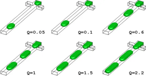
Fig.6shows the formation of plugs in the DCJ regime as a function of flow rate ratio for Ca¼0.002. The FIG. 5. (Color online) (a) Droplet flow regimes as a function of flow rate ratio Q and capillary number Ca (k¼1=6,

C¼1, andK¼2), where symbols indi-cate different regimes (~: DCJ,^: DC, andh: PF) and (b) representative drop-let formation atCa¼0.004 andQ¼0.6 (DCJ), 2.5 (DC), and 3 (PF). Note that the dash and dash-dot-dot lines in (a) are to clearly distinguish the different flow regimes.

monodisperse plugs are found to be regularly generated. The plug length increases withQ, and the formation of plugs will switch to the DC regime whenQis beyond 2.2. Also, the dis-tance between two neighboring plugs decreases when the flow rate ratio increases. Fig. 7 plots the non-dimensional length of plugs formed in the DCJ regime against the flow rate ratio forCa¼0.002, 0.004, 0.006, and 0.008. For each capillary number, our simulation results are found to obey the scaling law given by Eq.(29). Meanwhile, Eqs.(28)and (29)show that the plug lengths formed in the squeezing re-gime depend only on the flow rate ratio and are independent of the capillary number. However, it can be clearly seen from Fig.7that the fitting constants,eandx, are not solely determined by the channel geometry, and the plug lengths are indeed a function of capillary number.

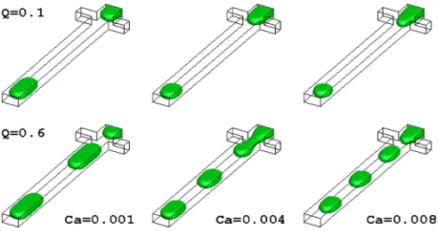
In order to explore the dependence of plug length on the capillary number, we measure the plug length as a function of capillary number at a fixed flow rate ratio. Three different flow rate ratiosQ¼0.1, 0.3, and 0.6 are examined, respec-tively. For each fixedQ, the capillary number is varied from 0.001 to 0.008. It should be noted that, here, a smaller capil-lary number (i.e., Ca¼0.001) is also simulated. However, the present computational domain is not large enough to sim-ulate the transition from DC to PF as the plug front may have moved out of the computational domain before the plug detaches from the long downstream jet in the DC regime.

Fig.8shows the formation of plugs as a function of cap-illary number forQ¼0.1 andQ¼0.6. For each fixedQ, the distance between two neighboring plugs and their size decrease with the increase of capillary number. Large flow ratio can lead to narrow distance between two neighboring plugs for the sameCa, which is consistent with the simula-tion results ofCa¼0.002 as shown in Fig. 6. Fig.9shows the simulation results of non-dimensional length of plugs versus capillary number for three different flow rate ratios.

Clearly, the non-dimensional length of plugs (L=wc) shows

no sign of approaching a constant value as the capillary num-ber decreases and exhibits a power-law dependence on the capillary number, i.e.,L=wc¼kCam, which is independent of

the flow rate ratio Q. The power-law behavior was also experimentally observed by Tan and his co-workers in microfluidic cross-junction18 and T-junction,58 where the formation of plugs occurred in the squeezing (DCJ) regime. Christopher et al.26 found that, in both squeezing and drip-ping regimes, the droplet volume exhibits a power-law de-pendence on the capillary number with a power-law exponent approximately equal to 0.3 at low viscosity ratio (k1=50).

Considering the influence of capillary number and flow rate ratio, the generated plug length can be predicted by

L wc

¼ ð~eþx~QÞCam~; (30)

where ~e, x, and~ m~ are the fitting parameters that mainly depend on the channel geometry. All of our numerical

FIG. 7. (Color online) Non-dimensional length of plugs versus the flow rate ratio forCa¼ f0.002, 0.004, 0.006, 0.008g,k¼1=6,C¼1, andK¼2 in the DCJ regime. Discrete symbols represent the simulation results. The lines are the fitting results of the scaling lawL=wc¼eþxQ.

FIG. 8. (Color online) Formation of plugs as a function of the capillary number forQ¼ f0.1, 0.6g,k¼1=6,C¼1, andK¼2 in the DCJ regime.

FIG. 9. (Color online) Non-dimensional length of plugs versus the capillary number for Q¼ f0.1, 0.3, 0.6g,k¼1=6,C¼1, andK¼2 in the DCJ re-gime. Discrete symbols represent the simulation results. Dashed-lines repre-sent the scaling law L

wc¼ ð~eþx~QÞCa ~

simulations confirm this scaling law and we can determine the coefficients as

L wc

¼ ð0:551þ0:277QÞCa0:292: (31)

To test our scaling law, the parity plot is used in which the predicted plug length is calculated by Eq.(30)and plotted as a function of our simulation results. The match between model predictions and simulation results is indicated by the scatter of data around the line of parity. The closer the data points are to the line of parity and the more even their distri-bution is, the better model predictions and simulations match. The predicted results of Eq. (30) show good agree-ment with our numerical simulations, as shown in Fig. 10. The fitting power-law exponentm~¼ 0:292 is very close to the experimental findings of Chiristopheret al.26in a T-junc-tion. Through the statistical analysis on the droplet formation in microfluidic T-junctions, Steegmans et al.30 found that none of the available scaling laws is general enough to describe the original data and the data from other literature sources. A two-step model was found to be statistically valid over the whole range of literature data. In their two-step model, the final droplet volume V is a result of two-stage growth, which is similar to the idea of Garsteckiet al.23 Ini-tially, the droplet grows to a critical volume Vc until the

forces exerted on the interface become balanced. Subse-quently, the droplet continues to grow for a timetnuntil final

pinches-off, due to the continuous injection of the dispersed phase fluid, so that the final droplet volume becomes

V¼VcþtnQd: (32)

Similar to Steegmans et al.,30 we also assume plugs enclosed between channel walls to be flat ellipses, so that Eq.(30)can be expressed as

V¼pwcwdh

4 ~eþ

~ x Qc

Qd

Cam~: (33)

It can be clearly seen that our scaling law given by Eq.(30) is consistent with the two-step model, i.e., Eq.(32)if

Vc¼ p

4wcwdh~eCa ~ m_;

tn ¼ p 4Qc

wcwdhx~Cam~: (34)

It is obvious that the necking time tnis associated with both

CaandQc. At a fixed capillary number, a large shear rate of

continuous phase is expected to shorten the necking time, leading to smaller droplets.

B. The influence ofKandC

To test whether the confinement of geometry plays an important role in the breakup of plugs,23,26,29 we examine the influence of the dimensionless geometrical parametersK andCon the length and shapes of the plugs. In the simula-tions, to single out the influence ofK,wcandhare kept

con-stant withC¼5=8. To study the influence ofC,wc andwd

are kept constant withK¼1. The fluid pair is fixed with the interfacial tension r¼0.06 and the viscosity ratio k¼0.3. To statistically obtain the scaling law given by Eq. (30)for each group of geometrical parameters, we carry out the nu-merical simulations withCa¼0.001, 0.0018, and 0.004, and the corresponding Reynolds number is 0.211, 0.38, and 0.844, respectively. For each fixedCa, we vary the flow rate ratio, i.e., Q¼ f0.05, 0.1, 0.25, 0.5, 1, 1.5gby varying the flow rate of the dispersed phase.

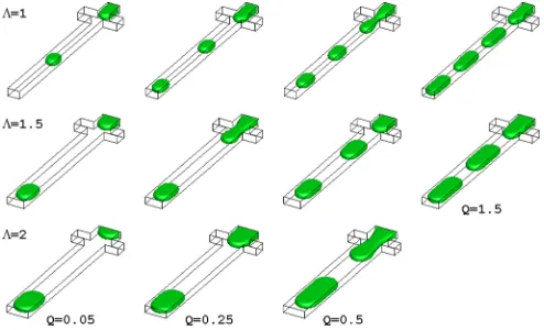
Fig.11shows the formation of plugs in the DCJ regime as a function of width ratio (K) atCa¼0.0018, Re¼0.38, and Q¼ f0.05, 0.25, 0.5, 1.5g. Three different width ratios are examined, i.e.,K¼1, 1.5, and 2, with the computational domain consisting of 2505711, 2506511, and 2507311 lattices, respectively. For each fixed flow rate ratio, the plug length increases with K (wd), which

corre-sponds to a more significant increase in the volume of plugs. Also, the increasingKcan enlarge the distance between two neighboring plugs. For each fixed width ratio, big flow rate ratio can lead to large plugs and narrow distance between consecutive plugs. We also notice that the plugs become

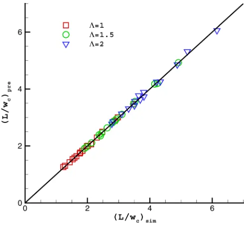
FIG. 10. (Color online) The parity plot of the non-dimensional length of plugs between the correlated resultsðL=wcÞprefrom Eq.(31)and the simula-tion resultsðL=wcÞsimforCa¼0.001, 0.002, 0.004, 0.006, and 0.008. The solid line represents the line of parity.

FIG. 11. (Color online) Formation of plugs as a function of the width ratio at various flow rate ratios in the DCJ regime withCa¼0.0018,Re¼0.38,

more and more difficult to “pinch-off” as the width ratio increases. For large values of K and Q, e.g., K¼2 and Q¼1.5, we find that the detachment point moves towards the downstream of the junction, so the DC regime starts. Therefore, it can be expected that transitions from DCJ to DC and from DC to PF occur at smaller flow rate ratios for a largeK.

The scaling law given in Eq. (30)is used to fit our nu-merical simulation results forK¼1, 1.5, and 2. Based on the least-square fitting, the resulting scaling equations can be expressed as _wL

c¼ ð0:32þ0:219QÞCa

0:243 _{for K¼1,}

L

wc¼ ð0:397þ0:21QÞCa

0:28 _{for K¼1.5, and} L

wc¼ ð0:788

þ0:521QÞCa0:222 forK¼2. Fig.12 gives the comparison of non-dimensional length of plugs between our simulation results and the predicted results forK¼1, 1.5, and 2. It can be clearly seen that the simulation results could be well described by our scaling law with the fitting parameters depending on the width ratio. Fig.13plots the non-dimen-sional length of plugs as a function of flow rate ratio at Ca¼0.0018, Re¼0.38, and C¼5=8 for three different width ratios. With the fixedCa of 0.0018, our scaling law, i.e., Eq.(30)reduces to Eq.(29). Specifically, they become

L

wc¼1:483þ1:015Q for K¼1, L

wc¼2:328þ1:232Q for K¼1.5, and _wL

c¼3:202þ2:115Q for K¼2, respectively. We can easily observe that the fitting constants eandx in Eq.(29)are both dependent on the width ratioK. Also, the values ofeandxincrease asKincreases.

Fig.14shows the non-dimensional length of plugs as a function of the width ratio forCa¼0.0018 and 0.0036. Con-sistent with the previous findings (see Figs. 7–9), the plug length decreases with the increase ofCafor the fixedKand Q. At small width ratio (K<1), the plug length is weakly de-pendent on the width ratio. When the width ratio is beyond 1, i.e.,K>1, the plug length is approximately linearly pro-portional to the width ratio. In addition, the simulation

results shown in Fig.14are in good agreement with the ex-perimental findings of Christopheret al.26for droplet genera-tion at T-juncgenera-tions. Fig. 15 gives the comparison of plug shapes for a broad range of width ratios with Q¼0.2 and Ca¼0.0036. It can be easily found that the width ratio can significantly influence the volume of plugs. The volume of plugs increases with the width ratio. Also, the increasing width ratio can enlarge the distance between two neighbor-ing plugs forK>1.

We also investigate the influence of Con the forma-tion of plugs at a fixed width ratio K¼1. We choose

FIG. 12. (Color online) The parity plot of non-dimensional length of plugs between the predicted resultsðL=wcÞpre from Eq.(30)and the simulation resultsðL=wcÞsimforK¼1, 1.5, and 2. The solid line represents the line of parity. The values of the fitting parameters in Eq.(30)are listed in the text.

FIG. 13. (Color online) The non-dimensional length of plugs versus the flow rate ratio forK¼ f1, 1.5, 2g,Ca¼0.0018,Re¼0.38, andC¼5=8 in the DCJ regime. The discrete symbols are the simulation results. The lines are the fitting results of the scaling lawL=wc¼eþxQ.

FIG. 14. (Color online) The non-dimensional length of plugs versus the width ratio at a fixed flow rate ratio Q¼0.2 and a fixed viscosity ratio

C¼ f5=8, 1, 5=4gwith the computational domain consist-ing of 2505711, 2505717, and 2505721 lat-tices, respectively. Fig.16shows the simulation results for C¼ f5=8, 1, 5=4g at Ca¼0.0018 and Re¼0.38 with a range of flow rate ratios. For each fixed flow rate ratio, the size of plugs increases asCincreases. In the same way, we use our scaling law (i.e., Eq. (30)) to fit the simulation data for each fixed C. The calculated scaling equations could be written as L

wc ¼ ð0:32þ0:219QÞCa

0:243 _for

C¼5=8, L

wc ¼ ð0:347 þ0:253QÞCa

0:245 _{for C¼1, and}

L

wc¼ ð0:36þ0:27QÞ Ca

0:255 _{for C¼5=4. The predicted}

results of these scaling equations all agree well with the simulation results, as can be shown in Fig.17. This indi-cates again that our scaling law is general enough to describe the size of plugs formed in the DCJ regime at microfluidic cross-junctions.

Fig. 18 shows the non-dimensional droplet length as a function of the flow rate ratio atCa¼0.0018,Re¼0.38, and K¼1 for three differentC. For each fixed channel depth, the non-dimensional length of plugs increases with the flow rate ratio, as observed in the previous cases. For the given capil-lary number, i.e.,Ca¼0.0018, the calculated scaling equa-tions can reduce to L

wc¼1:483þ1:015Q for C¼5=8, L

wc¼1:634þ1:191Q for C¼1, and L

wc ¼1:807þ1:353Q for C¼5=4. Obviously, both fitting parameters e and x depend onC, and they both increase asCincreases. A similar observation was reported by Gupta and Kumar59in

microflui-dic T-junctions. Our simulation results shown in Fig.18also indicate that the droplet behavior is expected to approach the scaling law of Eq.(28)as the channel depthhdecreases.

Although the scaling law of Eq.(30)developed from our simulation results is consistent with some experimental find-ings, we would like to more directly compare our simulations results with experimental data. Wu et al.36 experimentally reported droplet generation in a microfluidic cross-junction, where, unlike the other experimental work, they clearly gave FIG. 15. (Color online) Comparison of plug shapes for a broad range of

width ratio withQ¼0.2,Ca¼0.0036,Re¼0.76,k¼0.3, andC¼5=8 in the DCJ regime.

FIG. 16. (Color online) Formation of plugs as a function of height-to-width ratio forQ¼ f0.05, 0.25, 0.5, 1.5gwith Ca¼0.0018,Re¼0.38,k¼0.3, andK¼1 in the DCJ regime.

FIG. 17. (Color online) Parity plot of the non-dimensional length of plugs between the predicted resultsðL=wcÞpre from Eq.(30)and the simulation resultsðL=wcÞsimforC¼5=8, 1, and 5=4. The solid line represents the line of parity. The values of the fitting parameters in Eq.(30)are listed in the text.

the most of required physical and mechanical parameters for meaningful comparison. Our numerical simulations are per-formed withqN

S ¼ 1 and0.75 specified at the solid walls, corresponding to the static contact angleh180 and 160 , respectively. The other parameters are set to be the same as in Ref. 36. Table I shows that the simulation results with qN

S ¼ 0:75 are in good agreement with the experimental findings, while the simulations withqN

S ¼ 1 produce larger droplets. We also find that the droplet sizes obtained by our simulations can be described by Eq. (30) as L

wc ¼ ð0:58

þ0:358QÞCa0:255 _{for q}N

S ¼ 1 and wLc¼ ð0:645þ0:332QÞ Ca0:218 _forqN

S ¼ 0:75. For comparison, TableIalso gives the predicted results of non-dimensional droplet length using the scaling equation L

wc¼ ð0:645þ0:332QÞCa

0:218_.

Obvi-ously, the predicted results coincide with our simulation results qN

S ¼ 0:75

and the experimental data of Wuet al.36This indicates that our proposed scaling law can predict the correct droplet size generated in microfluidic cross-junctions.

Finally, we note that the droplet size exhibits a power-law dependence on the capillary number with the fitted power-law exponent ranging from0.3 to 0.2 for all the flow conditions and channel geometries in the present study. As we stated above, this power-law behavior has also been observed by some other authors. However, the values of the power-law exponent vary significantly in their observations. For example, Tan et al.18 and Xu et al.29 experimentally found that the plug length obeys L

wc /Ca

0:2 _{in a}

microflui-dic cross-junction and a microfluimicroflui-dic T-junction, while van der Graafet al.24numerically observed that, in both confined and unconfined droplet breakup at a T-junction, the final droplet volumeVcould be expressed asV/Ca0:75_.

Chris-topher et al.26 recently reported that the droplet volume V approximately follows V/Ca0:3 _{in the microfluidic}

T-junctions with C<1 and the viscosity ratio k 1=50. Herein, it should be noted that the droplet size is often expressed as volumeVwhich can be correlated to the plug length asV/ L

wcfor the plugs enclosed in a microchannel.

IV. CONCLUSIONS

The 3D lattice Boltzmann model has been applied to study the droplet formation in microfluidic cross-junctions

for low capillary numbers (Ca<0.01). Three different flow regimes as a consequence of interaction between two immis-cible fluids are identified to be dependent on the capillary number and the flow rates of the continuous and dispersed phases. A regime map is created to describe the transition from droplets formed at a cross-junction (DCJ), downstream of the cross-junction (DC), to stable PF. The influence of flow rate ratio, capillary number, and dimensionless geomet-rical parameters (KandC) is studied in detail with a broad range of flow conditions in the DCJ regime. The formation of plugs in the DCJ regime is shown to be dominated by the build-up of pressure that arises in the upstream when the emerging droplet interface obstructs the main channel. We observe that the length of the plugs is linearly proportional to the flow rate ratio for a fixed capillary number and exhibits a power-law dependence on the capillary number for a fixed flow rate ratio. Considering the effects of capillary number and flow rate ratio, an empirical scaling law is developed to predict the length of plugs. It is consistent with the two-step models proposed by van der Graaf et al.60 and Steegmans et al.30The channel geometry is found to play an important role in the process of plug breakup since the squeezing pres-sure becomes significant when the emerging dispersed-inter-face obstructs the main channel. At a fixed capillary number, our scaling law can reduce to the scaling equation proposed by Xuet al.,29i.e.,L=wc¼eþxQ. We find that the width

ra-tio (K) and the depth-to-width rara-tio (C) can affect the fitting constants eandx. Also, we find that the threshold value of flow rate ratio decreases with the width ratio, which distin-guishes the different flow regimes.

ACKNOWLEDGMENTS

The authors would like to thank Dr. Long Wu for the valuable discussions and Dr. Ian Halliday for providing us a version of his two-dimensional LB code.

1

D. Beebe, M. Wheeler, H. Zeringue, E. Walters, and S. Raty, “Microfluidic technology for assisted reproduction,”Theriogenology57, 125 (2002).

2

A. J. deMello, “Microfluidics: DNA amplification moves on,”Nature422, 28 (2003).

3_{G. F. Christopher and S. L. Anna, “Microfluidic methods for generating}

continuous droplet streams,”J. Phys. D: Appl. Phys.40, R319 (2007).

4

A. Huebner, S. Sharma, M. Srisa-Art, F. Hollfelder, J. B. Edel, and A. J. deMello, “Microdroplets: A sea of applications?,”Lab Chip8, 1244 (2008).

5_{B. Zheng, L. S. Roach, and R. F. Ismagilov, “Screening of protein}

crystal-lization conditions on a microfluidic chip using nanoliter-size droplets,”J. Am. Chem. Soc.125, 11170 (2003).

6

H. Song, D. L. Chen, and R. F. Ismagilov, “Reactions in droplets in micro-fluidic channels,”Angew. Chem. Int. Ed.45, 7336 (2006).

7_{S. Sugiura, M. Nakajima, H. Itou, and M. Seki, “Synthesis of polymeric}

microspheres with narrow size distributions employing microchannel emulsification,”Macromol. Rapid Commun.22, 773 (2001).

8_{D. Dendukuri, K. Tsoi, T. A. Hatton, and P. S. Doyle, “Controlled}

synthe-sis of nonspherical microparticles using microfluidics,” Langmuir 21, 2113 (2005).

9

V. Srinivasan, V. K. Pamula, and R. B. Fair, “Droplet-based microfluidic lab-on-a-chip for glucose detection,”Anal. Chim. Acta507, 145 (2004).

10_{J. Khandurina, T. E. McKnight, S. C. Jacobson, L. C. Waters, R. S. Foote,}

and J. M. Ramsey, “Integrated system for rapid PCR-based DNA analysis in microfluidic devices,”Anal. Chem.72, 2995 (2000).

11_{N. Bontoux, A. Pe´pin, Y. Chen, A. Ajdari, and H. A. Stone, “Experimental}

characterization of hydrodynamic dispersion in shallow microchannels,” Lab Chip6, 930 (2006).

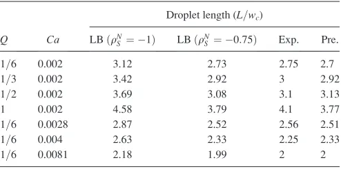
TABLE I. Non-dimensional droplet length obtained from the experiment (Ref.36) and our simulations withqN

S ¼ 1 and0.75 at various flow rate ratios and capillary numbers. For comparison, we also give the predicted values of non-dimensional droplet length using the scaling equation

L

wc¼ ð0:645þ0:332QÞCa

0:218_{. Note: our definition ofCais different from}

Ref.36.

Droplet length (L=wc)

Q Ca LBðqN

S ¼ 1Þ LBðqNS ¼ 0:75Þ Exp. Pre.

1=6 0.002 3.12 2.73 2.75 2.7

1=3 0.002 3.42 2.92 3 2.92

1=2 0.002 3.69 3.08 3.1 3.13

1 0.002 4.58 3.79 4.1 3.77

1=6 0.0028 2.87 2.52 2.56 2.51

1=6 0.004 2.63 2.33 2.25 2.33

12

J. D. Tice, H. Song, A. D. Lyon, and R. F. Ismagilov, “Formation of drop-lets and mixing in multiphase microfluidics at low values of the Reynolds and the Capillary numbers,”Langmuir19, 9127 (2003).

13_{M. Yasuno, S. Sugiura, S. Iwamoto, M. Nakajima, A. Shono, and K.}

Satoh, “Monodispersed microbubble formation using microchannel technique,”AIChE J.50, 3227 (2004).

14

S. Sugiura, M. Nakajima, and M. Seki, “Prediction of droplet diameter for microchannel emulsification: Prediction model for complicated micro-channel geometries,”Ind. Eng. Chem. Res.43, 8233 (2004).

15

S. L. Anna, N. Bontoux, and H. A. Stone, “Formation of dispersions using ‘flow focusing’ in microchannels,”Appl. Phys. Lett.82, 364 (2003).

16_{T. Cubaud, M. Tatineni, X. Zhong, and C.-M. Ho, “Bubble dispenser in}

microfluidic devices,”Phys. Rev. E72, 037302 (2005).

17

P. Garstecki, H. A. Stone, and G. M. Whitesides, “Mechanism for flow-rate controlled breakup in confined geometries: A route to monodisperse emulsions,”Phys. Rev. Lett.94, 164501 (2005).

18_{J. Tan, J. Xu, S. Li, and G. Luo, “Drop dispenser in a cross-junction}

micro-fluidic device: Scaling and mechanism of break-up,”Chem. Eng. J.136, 306 (2008).

19_{T. Fu, Y. Ma, D. Funfschilling, and H. Z. Li, “Bubble formation and}

breakup mechanism in a microfluidic flow-focusing device,”Chem. Eng. Sci.64(10), 2392 (2009).

20

T. Thorsen, R. W. Roberts, F. H. Arnold, and S. R. Quake, “Dynamic pat-tern formation in a vesicle-generating microfluidic device,”Phys. Rev. Lett.86, 4163 (2001).

21

T. Nisisako, T. Torii, and T. Higuchi, “Droplet formation in a microchan-nel network,”Lab Chip2, 24 (2002).

22_{P. Guillot and A. Colin, “Stability of parallel flows in a microchannel after}

a T junction,”Phys. Rev. E72, 066301 (2005).

23

P. Garstecki, M. J. Fuerstman, H. A. Stone, and G. M. Whitesides, “Formation of droplets and bubbles in a microfluidic T-junction–scaling and mechanism of break-up,”Lab Chip6, 437 (2006).

24_{S. van der Graaf, T. Nisisako, C. G. P. H. Schroe¨n, R. G. M. van der}

Sman, and R. M. Boom, “Lattice Boltzmann simulations of droplet forma-tion in a T-shaped microchannel,”Langmuir22, 4144 (2006).

25_{M. D. Menech, P. Garstecki, F. Jousse, and H. A. Stone, “Transition from}

squeezing to dripping in a microfluidic T-shaped junction,”J. Fluid Mech. 595, 141 (2008).

26

G. F. Christopher, N. N. Noharuddin, J. A. Taylor, and S. L. Anna, “Experimental observations of the squeezing-to-dripping transition in T-shaped microfluidic junctions,”Phys. Rev. E78, 036317 (2008).

27

P. B. Umbanhowar, V. Prasad, and D. A. Weitz, “Monodisperse emulsion gen-eration via drop break off in a coflowing stream,”Langmuir16, 347 (2000).

28_{J. Hua, B. Zhang, and J. Lou, “Numerical simulation of microdroplet}

for-mation in coflowing immiscible liquids,”AIChE J.53, 2534 (2007).

29

J. Xu, S. Li, J. Tan, and G. Luo, “Correlations of droplet formation in T-junction microfluidic devices: From squeezing to dripping,”Microfluid. Nanofluid.5, 711 (2008).

30_{M. Steegmans, C. Schron, and R. Boom, “Generalised insights in droplet}

formation at T-junctions through statistical analysis,” Chem. Eng. Sci. 64(13), 3042 (2009).

31_{W. Shyy, R. W. Smith, H. S. Udaykumar, and M. M. Rao,Computational}

Fluid Dynamics with Moving Boundaries(Taylor & Francis, Washington, DC, 1996).

32

S. Succi,The Lattice Boltzmann Equation for Fluid Dynamics and Beyond (Oxford University Press, Oxford, 2001).

33

X. He and L.-S. Luo, “A priori derivation of the lattice Boltzmann equa-tion,”Phys. Rev. E55, R6333 (1997).

34

M. M. Dupin, I. Halliday, and C. M. Care, “Simulation of a microfluidic flow-focusing device,”Phys. Rev. E73, 055701 (2006).

35_{Z. Yu, O. Hemminger, and L.-S. Fan, “Experiment and lattice Boltzmann}

simulation of two-phase gas-liquid flows in microchannels,”Chem. Eng. Sci.62, 7172 (2007).

36

L. Wu, M. Tsutahara, L. S. Kim, and M. Ha, “Three-dimensional lattice Boltzmann simulations of droplet formation in a cross-junction micro-channel,”Int. J. Multiphase Flow34, 852 (2008).

37_{H. Liu and Y. Zhang, “Droplet formation in a T-shaped microfluidic}

junction,”J. Appl. Phys.106, 034906 (2009).

38

S. Chen and G. D. Doolen, “Lattice Boltzmann method for fluid flows,” Annu. Rev. Fluid Mech.30(1), 329 (1998).

39_{A. K. Gunstensen, D. H. Rothman, S. Zaleski, and G. Zanetti, “Lattice}

Boltzmann model of immiscible fluids,”Phys. Rev. A43(8), 4320 (1991).

40

X. Shan and H. Chen, “Lattice Boltzmann model for simulating flows with multiple phases and components,”Phys. Rev. E47(3), 1815 (1993).

41_{M. R. Swift, W. R. Osborn, and J. M. Yeomans, “Lattice Boltzmann}

simu-lation of nonideal fluids,”Phys. Rev. Lett.75(5), 830 (1995).

42

M. R. Swift, E. Orlandini, W. R. Osborn, and J. M. Yeomans, “Lattice Boltzmann simulations of liquid-gas and binary fluid systems,”Phys. Rev. E54(5), 5041 (1996).

43_{P. Yuan and L. Schaefer, “Equations of state in a lattice Boltzmann}

mod-el,”Phys. Fluids18, 042101 (2006).

44

M. Sbragaglia, R. Benzi, L. Biferale, S. Succi, K. Sugiyama, and F. Toschi, “Generalized lattice Boltzmann method with multirange pseudopotential,”Phys. Rev. E75(2), 026702 (2007).

45

A. L. Kupershtokh, D. A. Medvedev, and D. I. Karpov, “On equations of state in a lattice Boltzmann method,” Comput. Math. Appl. 58, 965 (2009).

46_{S. V. Lishchuk, C. M. Care, and I. Halliday, “Lattice Boltzmann algorithm}

for surface tension with greatly reduced microcurrents,”Phys. Rev. E67, 036701 (2003).

47_{M. Latva-Kokko and D. H. Rothman, “Diffusion properties of}

gradient-based lattice Boltzmann models of immiscible fluids,”Phys. Rev. E71, 056702 (2005).

48

I. Halliday, R. Law, C. M. Care, and A. Hollis, “Improved simulation of drop dynamics in a shear flow at low Reynolds and capillary number,” Phys. Rev. E73(5), 056708 (2006).

49

J. U. Brackbill, D. B. Kothe, and C. Zemach, “A continuum method for modeling surface tension,”J. Comput. Phys.100(2), 335 (1992).

50_{I. Halliday, A. P. Hollis, and C. M. Care, “Lattice Boltzmann algorithm}

for continuum multicomponent flow,”Phys. Rev. E76, 026708 (2007).

51

G. I. Taylor, “The viscosity of a fluid containing small drops of another fluid,”Proc. R. Soc. London, Ser. A138, 41 (1932).

52_{Q. Zou and X. He, “On pressure and velocity boundary conditions for the}

lattice Boltzmann BGK model,”Phys. Fluids9, 1591 (1997).

53

J. S. Rowlinson and B. Widom,Molecular Theory of Capillarity (Claren-don, Lon(Claren-don, 1989).

54_{S. Bekri and P. M. Adler, “Dispersion in multiphase flow through porous}

media,”Int. J. Multiphase Flow28(4), 665 (2002).

55

A. Briant, P. Papatzacos, and J. Yeomans, “Lattice Boltzmann simulations of contact line motion in a liquid-gas system,”Philos. Trans. R. Soc. Lon-don Ser. A360, 485 (2002).

56_{T. Lee and L. Liu, “Lattice Boltzmann simulations of micron-scale drop}

impact on dry surfaces,”J. Comput. Phys.229(20), 8045 (2010).

57

J. D. Tice, A. D. Lyon, and R. F. Ismagilov, “Effects of viscosity on drop-let formation and mixing in microfluidic channels,”Anal. Chim. Acta507, 73 (2004).

58

J. Tan, S. Li, K. Wang, and G. Luo, “Gas-liquid flow in T-junction micro-fluidic devices with a new perpendicular rupturing flow route,” Chem. Eng. J.146(3), 428 (2009).

59

A. Gupta and R. Kumar, “Effect of geometry on droplet formation in the squeezing regime in a microfluidic T-junction,” Microfluid. Nanofluid. 8(6), 799 (2010).

60_{S. van der Graaf, M. L. J. Steegmans, R. G. M. van der Sman, C. G. P. H.}