Impact of source model matrix conditioning on PEVD algorithms
J Corr
∗, K Thompson
∗, S Weiss
∗, I K Proudler
†, J G McWhirter
‡∗Department of Electronic and Electrical Engineering, University of Strathclyde, Glasgow, Scotland †School of Electronic, Electrical and Systems Engineering, Loughborough University, Loughborough, UK
‡School of Engineering, Cardiff University, Cardiff, Wales, UK
{jamie.corr,keith.thompson,stephan.weiss}@strath.ac.uk
Keywords: broadband array processing; space-time covari-ance matrix; polynomial matrix; matrix factorisation; polyno-mial eigenvalue decomposition.
Abstract
Polynomial parahermitian matrices can accurately and ele-gantly capture the space-time covariance in broadband array problems. To factorise such matrices, a number of polyno-mial EVD (PEVD) algorithms have been suggested. At every step, these algorithms move various amounts of off-diagonal energy onto the diagonal, to eventually reach an approximate diagonalisation. In practical experiments, we have found that the relative performance of these algorithms depends quite significantly on the type of parahermitian matrix that is to be factorised. This paper aims to explore this performance space, and to provide some insight into the characteristics of PEVD algorithms.
1. Introduction
Parahermitian polynomial matrices can compactly characterise quantities such as space-time covariance matrices in broad-band array problems. Based on a data vectorx[n]∈ CM, the
space-time covarianceR[τ] = Ex[n]xH[n] , withE{·}the expectation operator, leads to a polynomial matrix represen-tation for its z-transform,R(z) = PτR[τ]z−τ. This
cross-spectral density matrix R(z) is parahermitian, i.e. R˜(z) =
RH(z−1) =R(z), where the parahermitian operator{·}˜ per-forms a complex conjugate transpose and time reversal of all matrix entries.
To extend the utility of the eigenvalue (EVD) and singu-lar value decompositions (SVD) [1] to general broadband problems, a polynomial EVD (PEVD [2–4]) has been defined. Given a parahermitianR(z), the PEVD
R(z)≈Q˜(z)Λ(z)Q(z) , (1)
results in paraunitary factorsQ(z)and a diagonal, spectrally majorised and parahermitian Λ(z). The latter contains the polynomial eigenvalues,
Λ(z) =diag{Λ1(z) Λ2(z) . . . ΛM(z)} . (2)
with spectral majorisation enforcing an ordering such that
Λm+1(ejΩ)≥Λm(ejΩ), ∀Ω, m= 1. . . M−1 . (3)
Paraunitarity ofQ(z)implies thatQ(z) ˜Q(z) = ˜Q(z)Q(z) =
I. While equality in (1) is not guaranteed, the approximation has been suggested to hold close for sufficiently high orders of Q(z)[5].
A number of PEVD algorithms have been introduced [4,6– 10], and offer various performance characteristics. The algorithms in [4,6,10] have been demonstrated on para-hermitian matrices R(z) ∈ CM×M derived from random
A(z) ∈ CM×K asR(z) = A(z) ˜A(z). ForK < M,R(z)
is guaranteed to be rank deficient, but when K ≥ M it is possible forR(z) to have full rank. In [7,8], subband cod-ing was considered as an application, and the parahermitian matrices that need to be factorised by the algorithms were based on auto-regressive functions generating auto-correlation functions with infinite support but potentially permitting finite order paraunitary factors (for a justification, see the factorisa-tion in Sec. IV.B.3 in [8]). In [9], a source model convolutively mixes spectrally majorised sources by means of an arbitrary paraunitary matrix, such that the ground truth PEVD with finite order factors and equality in (1) is guaranteed. Since these publications [4,6–10] use differently conditioned prob-lems, a direct comparison between algorithms proposed in individual papers is not always straightforward.
In this paper, we generalise the source model idea in [9] to carefully control the conditioning of the parahermitian matrix. This includes a definition of the dynamic range of the under-lying source, which can be linked to the condition number or eigenvalue spread of a parahermitian matrix by generalisation from the field of scalar matrices. Besides the dynamic range, we also define different relations between of the sources’ PSDs. These may be
• not spectrally majorised (i.e. with overlapping PSDs); • spectrally majorised, with ’≥’ in (3), or
• strictly spectrally majorised, with ’>’ in (3).
An ensemble of randomised parahermitian matrices with dif-ferent dynamic ranges and types of majorisation are factorised by a number of PEVD algorithms belonging to the second order sequential best rotation (SBR2 family, [4,8] and the sequential matrix diagonalisation (SMD family, [9,10]).
belonging to the SBR2 and SMD families. Sec. 3 shows the impact of the type of source majorisation on the order to the factors of the ground-truth PEVD, and introduces the condition number as a metric for the dynamic range of a parahermitian matrix. Experimental results for applying the various PEVD algorithms to differently conditioned parahermitian matrices are discussed in Sec. 4, followed by conclusions in Sec. 5.
2. PEVD Algorithms
2.1 General Anatomy
The current most popular PEVD algorithms [4,8–10] have the goal of diagonalising a parahermitian matrix R(z) starting from an initial approximation S(0)(z). The ith iteration of all algorithms consists of three common steps operating on S(i−1)(z), which vary with implementation.
In the first step of the i-th iteration, the remaining off-diagonal elements of the parahermitian matrixS(i−1)(z)are searched. Part of the off-diagonal energy is then transferred onto the zero lag in the second step using a paraunitary shift matrix,
S(i)′(z) =Λ(i)(z)S(i−1)(z) ˜Λ(i)(z), i= 1. . . I . (4)
The search step and therefore the construction of the shift matrix,Λ(i)(z), depend on the particular PEVD implementa-tion as detailed below. The final step in theith iteration is to bring the off-diagonal energy, found in step one and shifted in step two, onto the diagonal of the zero lag matrix. This is accomplished by means of a unitary matrix, Q(i), which is applied to all lags in the parahermitian matrix,S(i)′(z), such that
S(i)(z) =Q(i)S(i)′(z)Q(i)H . (5)
Like the shift matrix,Λ(i)(z), the construction of the unitary energy transfer matrix, Q(i), depends on the specific PEVD algorithm.
The PEVD algorithm is complete when either a set num-ber of iterations,I, have been carried out or the search step returns an amount of energy lower than a predefined thresh-old. Upon completion, the PEVD algorithm returns the approx-imate polynomial eigenvalues in the diagonalised parahermi-tianS(I)(z)and the approximate polynomial eigenvectors in Q(I)(z). The polynomial eigenvectors are simply the product of the unitary energy transfer matrices,Q(i), and paraunitary shift matrices,Λ(i)(z), from each of theIiterations,
Q(I)(z) =G(I)(z). . .G(2)(z)G(1)(z) , (6)
where the paraunitary matrix G(i) is constructed from the energy transfer and shift matrices i.e.
G(i)(z) =Q(i)Λ(i)(z) . (7)
To reduce the computational cost of applying the paraunitary matrix,Q(I)(z), a paraunitary trim function is used to signif-icantly reduce the polynomial order ofQ(I)(z). In this paper we use the recently developed row-shift corrected truncation method [11], this approach takes advantage of an ambiguity in the paraunitary matrix to further reduce its polynomial order.
2.2 Second Order Sequential Best Rotation
With the initialisation S(0)(z) = R(z), the first step of the SBR2 algorithm [4] at theith iteration utilises a search for the off-diagonal element with the largest modulus,
{k(i), τ(i)}= arg max
k,τ kˆs
(i−1)
k [τ]k∞, i= 1. . . I , (8)
where the modified column vector,ˆs(ki−1)[τ], contains all ele-ments apart from the on-diagonal entries. Based on the column and lag indices,k(i)andτ(i)respectively, the paraunitary shift matrix,Λ(i)(z), is then generated as
Λ(i)(z) = diag{1 . . . 1 | {z }
k(i)−1
z−τ(
i)
1 . . . 1 | {z }
M−k(i)
} . (9)
The maximum element found in (8) and shifted onto the zero lag using (9) is transferred onto the diagonal using a Jacobi rotation forQ(i)in (5). The sparse nature of the Jacobi rota-tion means that rather than applying a full matrix multiplica-tion to each lag in the parahermitian matrix, only two rows and columns ofS(i)′(z)are affected across all its lags.
2.3 Sequential Matrix Diagonalisation
The SMD algorithm [9] includes an initialisation step which diagonalises the zero lag of the parahermitian matrix,
S(0)[0] =Q(0)R[0]Q(0)H . (10)
In (10) the unitary matrix,Q(0), is the modal matrix from the EVD ofR[0]which brings all the energy in the zero lag onto the diagonal, zeroing the off-diagonal elements. As withQ(i) in (5),Q(0)is applied to all lags of the parahermitian matrix, such thatS(0)(z) =Q(0)R(z)Q(0)H.
The i-th iteration of the SMD algorithm starts with the search for the maximum column norm,
{k(i), τ(i)}= arg max
k,τ kˆs
(i−1)
k [τ]k2, i= 1. . . I . (11)
Using thel2norm differs from (8), which extracts the maxi-mum element (i.e. thel∞norm). Like SBR2, the shift step in
the SMD approach uses (9) to construct the paraunitary shift matrixΛ(i)(z).
Rather than transferring the energy from a single element onto the diagonal like SBR2, the SMD algorithm uses the modal matrix of the EVD of the new zero lag, similar to (10), to constructQ(i)and transfer all the zero lag energy onto the diagonal. Typically the SMD algorithm will transfer a greater amount of energy onto the diagonal than SBR2 at each iter-ation. The main drawback of the SMD algorithm is the cost associated with applying the non-sparse Q(i) to the entire parahermitian matrix at each iteration.
2.4 Multiple Shift Maximum Element SMD
The MSME-SMD algorithm [10] employs the same initialisa-tion step as the SMD algorithm above to bring the zero lag energy onto the diagonal. At each iteration, the SMD’sl2 col-umn norm search is replaced by a maximum element search as in (8). Whereas the SMD algorithm immediately diagonalises the energy brought onto the zero lag matrix, the MSME-SMD algorithm uses a set of reduced search spaces, detailed in [10], to bring a total ofM−1maximum elements onto the zero lag at each iteration, whereMis the spatial dimension of the para-hermitian matrix. The reduced search spaces have a dual pur-pose: firstly they ensure that previous maxima transferred onto the zero lag are not undone by subsequent shifts; secondly they are designed to guarantee that a total ofM −1elements are brought onto the zero lag at each iteration.
To bring theM −1maximum elements onto the zero lag, the paraunitary delay matrix,Λ(i)(z), must be modified to be
Λ(i)(z) =diagnz−τ(
i) 1 z−τ
(i)
2 . . . z−τ (i)
M
o
. (12)
The paraunitary delay matrix in (12) allows each of theMrows and columns of the parahermitian matrix to be advanced or delayed.
The MSME-SMD algorithm uses the same technique as SMD to transfer onto the diagonal, energy from all the ele-ments shifted onto the zero lag. Using the multiple shifts the MSME-SMD algorithm will bring more energy onto the zero lag at each iteration than the SMD equivalent. The compu-tational cost of one MSME-SMD iteration is slightly higher than SMD but the cost is dominated by by applying the modal matrix to all lags so the additional cost is not significant. Thus overall the higher energy transfer of MSME-SMD is more beneficial for real time convergence. A drawback of MSME-SMD compared to both SBR2 and MSME-SMD is that the order of the paraunitary and parahermitian matrices associated with the PEVD will grow faster.
3. Source Model Conditioning
For the analysis and simulations in this paper, we assume that the parahermitian matrices have a known ground truth decom-position. This enables us to control the condition of the prob-lem that is addressed by the various PEVD algorithms, and also assess and compare the solution that is reached.
3.1 Source Model
The general model is depicted in Fig. 1. A total of L inde-pendent source signals with individual power spectral densi-ties (PSDs)Fl(z) ˜Fl(z),l = 1. . . L, are generated by exciting innovation filtersFl(z)with unit variance zero-mean uncorre-lated complex Gaussian sourcesul[n][12]. The order of the innovation filters Fl(z) is P, and careful control of the fil-ter gain and the maximum radius of zeros can defil-termine the dynamic range of the source and whether they e.g. are spec-trally majorised as in [9]. Convolutive mixing of the source signals is performed by a random paraunitary matrixA(z)∈
A(z)
u1[n]
u2[n]
uL[n]
F1(z)
F2(z)
FL(z)
x1[n]
x2[n]
xM[n]
..
[image:3.595.343.517.92.171.2]. ... ...
Figure 1. Source model withLunit variance zero mean uncorrelated
com-plex Gaussian excitations ul[n], innovation filters with transfer functions
Fl(z),l = 1. . . L, followed by a paraunitary convolutive mixing system A(z).
CM×Lof orderK, withM ≥L. This matrix is determined by
extractingLcolumns from
A′(z) = K Y
k=1
(I−vkvHk +vkvHkz−1), (13)
which is a product ofK elementary paraunitary matrices [3], withvk∈CM,k= 1. . . K, being random unit norm vectors.
The space-time covariance matrix constructed from the out-putxT[n] = [x1[n] . . . xM[n]]is therefore given as
R(z) =X τ
Ex[n]xH[n−τ] z−τ (14)
=A(z)F(z) ˜F(z) ˜A(z). (15)
The diagonal matrixF(z) =diag{F1(z). . . FL(z)}contains theLinnovation filters.
3.2 Polynomial Eigenvalue Decomposition
Given that the parahermitian matrix in (15) is factorised into paraunitary and diagonal parahermitian matrices, it bears close relation with the PEVD (1) of R(z). If F(z) is spectrally majorised, then indeed the PEVDR(z) = Q(z)Λ(z) ˜Q(z)
exists with equality and is given by Q(z) = A(z) and Λ(z) =F(z) ˜F(z).
If F(z) is not spectrally majorised, then a PEVD satisfy-ing both diagonalisation and spectral majorisation could be derived by re-assigning spectral components of F(z) via a paraunitary matrix U(z) such that U(z)F(z) is spectrally majorised. For this, the filters inU(z) would ideally imple-ment a binary mask. Then Λ(z) = U(z)F(z) ˜F(z) ˜U(z), andU(z)can be absorbed intoA(z)to yield the polynomial modal matrixQ(z) = A(z) ˜U(z). Since an ideal U(z) pro-viding a binary spectral mask will require infinite support, the order of the factorsQ(z)andΛ(z)is likely to be much higher than in the spectrally majorised case.
Example. Let L = M = 2 with a diagonal F(z) =
diag1 +z−1; 1−z−1 generating the unmajorised PSDs in Fig. 2. IfUij(z),i, j ∈ {1,2}, are the elements of a matrix U(z)to enforce spectral majorisation, thenU11(z)andU22(z) must be halfband lowpass andU12(z)and U21(z)halfband highpass filters. If selected as quadrature mirror filters with U21(z) =−U12˜ (z)andU22(z) = ˜U11(z), the condition of paraunitarity reduces to demand power complementarity,
0 0.05 0.1 0.15 0.2 0.25 0.3 0.35 0.4 0.45 0.5 0
1 2 3 4
normalised angular frequency Ω/[2π]
PSDs
[image:4.595.53.300.97.183.2]original Haar 32C channel 1 channel 2
Figure 2. PSDs of unmajorised sources, and after frequency-reassignment using paraunitary matrices based on Haar [13] and 32C filters [14].
−2 0 2
0 1 2 3
−2 0 2
0 1 2 3
−2 0 2
0 1 2 3
−2 0 2
0 1 2 3
U1
(
z
)
F
(
z
)
˜F(
z
)
˜U1
(
z
)
coefficients (a)
−20 0 20
0 1 2 3
−20 0 20
0 1 2 3
−20 0 20
0 1 2 3
−20 0 20
0 1 2 3
U2
(
z
)
F
(
z
)
˜F(
z
)
˜U2
(
z
)
coefficients (b)
Figure 3. Approximately diagonalised matrices for paraunitary systems based on (a) Haar [13] and (b) 32C filters [14].
ForU(z)F(z) ˜F(z) ˜U(z)to retain a diagonal structure, it can be shown that
U11(z)U12(z)F1(z) ˜F1(z) =U11(z)U12(z)F2(z) ˜F2(z) (17)
is also required. This can be achieved only ifU11(z)U12(z) =
0, i.e. they are ideal, complementary, infinite length halfband lowpass and highpass filters.
Using a Haar filter [13] of order 1 to constructU1(z), the PSDs along the diagonal are now spectrally majorised as evi-dent from Fig. 2. However, inspectingU1(z)F(z) ˜F(z) ˜U1(z) in Fig. 3(a), (17) is violated resulting in off-diagonal terms. Using the filter 32C from [14] to construct an approximately paraunitary U2(z), the higher order of 31 now results in an approximately diagonalised U2(z)F(z) ˜F(z) ˜U2(z) as demonstrated in Fig. 3(b), which is also spectrally majorised according to Fig. 2.
Therefore if sources contributing toR(z)are not spectrally majorised, a PEVD ofR(z)in the sense of the definition in (1)–(3) requires higher order polynomial matrix factors than for a case where sources are spectrally majorised.
3.3 Eigenvalue Spread
Since PEVD algorithms have a stopping criterion that is tied to a threshold for off-diagonal values, the resolution of sources depends on the dynamic range of the source signals. There-fore, this dynamic range can be defined as the ratio between the maximum and minimum value across all source PSDs and frequencies,
γ=maxΩ,l|Fl(e
jΩ)|2
minΩ,l|Fl(ejΩ)|2
. (18)
ForM =L, even in the case where sources are not spectrally majorised, (18) represents a polynomial matrix condition
num-ber,
γ= maxΩΛ1(e
jΩ)
minΩΛM(ejΩ)
, (19)
as after re-assigning frequency bands between channels, the minimum and maximum PSD values remain unaltered as demonstrated in Sec. 3.2.
4. Results
The following subsections present the details of the simulation scenario followed by the performance metrics used to compare the different source models and PEVD algorithms. The final three subsections present and analyse the results of the simula-tions.
4.1 Performance Metrics
To assess the impact of source model conditioning on PEVD performance we use the following metrics. First the conver-gence of the PEVD algorithms is monitored via the normalised off-diagonal energy at thei-th iteration,
Enorm(i) = P
τ
PM
k=1kˆs
(i)
k [τ]k
2 2
P
τkR[τ]k2F
, (20)
whereˆs(ki)[τ]is the same modified column vector used in (8) and the denominator consists of the sum of Frobenius norms, k · kF, of the initial parahermitian matrix,R[τ], for each of the
τlags.
As well as noting Enorm(i) for every iteration, the order of the truncated paraunitary matrices is recorded to show how the source model affects the growth of the paraunitary matrix, which directly represents the implementation cost of this loss-less filter bank.
To compare the diagonal matrices produced by the PEVD to the ground truth of the source model we use the PSDs. Ideally the PSDs extracted by PEVD algorithms should match those of the source model, bar any frequency-reassignments in the case of spectrally unmajorised sources.
4.2 Simulation Scenarios
The first two sets of simulations present the results from
500iterations of the PEVD algorithms outlined in Sec. 2 for the spectrally majorised and ummajorised examples over an ensemble of102 random instantiations. WithL = 4sources acquired byM = 4sensors, for each instantiation the source model produces a distinct parahermitian matrix,R(z)∈C4×4.
WithP =K= 30, the order ofR(z)is 120. For each ensem-ble, restrictions on the radii of zeros in the innovation filters create an average dynamic range of either10or20dB.
[image:4.595.52.301.234.332.2]0 50 100 150 200 250 300 350 400 450 500 −30
−25 −20 −15 −10 −5
iteration indexi
5
lo
g10
E
{
E
(
i
)
n
o
rm
}
/
[d
B
] SBR2
[image:5.595.44.291.98.189.2]SMD MSME−SMD Unmajorised Strict Majorised
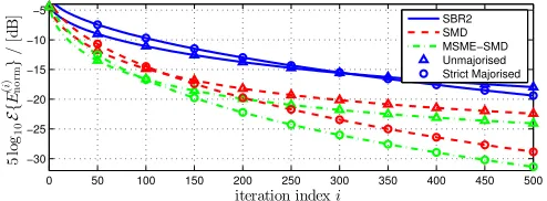
Figure 4. Reduction in off diagonal energy for both majorisation types with a dynamic range of 10 dB for a selection of PEVD algorithms.
0 50 100 150 200 250 300 350 400 450 500
−30 −25 −20 −15 −10 −5
iteration indexi
5
lo
g10
E
{
E
(
i
)
n
o
rm
}
/
[d
B
] SBR2
[image:5.595.307.551.98.190.2]SMD MSME−SMD Unmajorised Strict Majorised
Figure 5. Reduction in off diagonal energy for both majorisation types with a dynamic range of 20 dB for a selection of PEVD algorithms.
4.3 Algorithm Convergence
Figs. 4 and 5 show how the different algorithms converge for the two source models identified in Sec. 3 for dynamic ranges of 10 dB and 20 dB respectively. In both Figs. 4 and 5 all algorithms initially converge faster for the unmajorised source but as the number of iterations increases, these curves slow down and are overtaken by the strictly majorised sources. After 500 iterations there is a noticeable difference between the two source models, with the strictly majorised being better; this is apparent for both dynamic ranges and all three PEVD algo-rithms. With the higher dynamic range in Fig. 5 we can see that the curves all appear worse than their counterparts in Fig. 4 and end up closer together.
4.4 Paraunitary Order
The growth in paraunitary order for the PEVD methods using the unmajorised and strictly majorised sources at 10 dB is shown in Fig. 6 with the larger dynamic range of 20 dB depicted in Fig. 7. In both Figs. 6 and 7 the SMD and SBR2 algorithms perform similarly but the multiple shifts of the MSME-SMD algorithm cause the paraunitary order to grow faster. The paraunitary order for the MSME-SMD algo-rithm is also affected more when the dynamic range of the source increases. For all the algorithms over both dynamic ranges we see that the paraunitary orders for the unmajorised sources tends be higher than the strictly majorised source. The main exception to this is the MSME-SMD with the strictly majorised (20dB) source where it mostly performs worse than its unmajorised equivalent.
4.5 Power Spectral Densities
This section investigates four example source models which have had the SMD algorithm applied for 100 iterations each.
0 20 40 60 80 100 120 140 160 180 200 220
−30 −25 −20 −15 −10 −5
paraunitary order
5
lo
g10
E
{
E
(
i
)
n
o
rm
}
/
[d
B
] SBR2
SMD MSME−SMD Unmajorised Strict Majorised
Figure 6. Paraunitary matrix order for both majorisation types with a dynamic range of 10 dB for a selection of PEVD algorithms.
0 20 40 60 80 100 120 140 160 180 200 220
−30 −25 −20 −15 −10 −5
paraunitary order
5
lo
g10
E
{
E
(
i
)
n
o
rm
}
/
[d
B
] SBR2
[image:5.595.45.291.226.318.2]SMD MSME−SMD Unmajorised Strict Majorised
Figure 7. Paraunitary matrix order for both majorisation types with a dynamic range of 20 dB for a selection of PEVD algorithms.
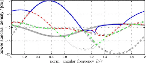
PSDs of the source models are shown in Figs. 8,9,10 and 11, first showing a10dB dynamic range for the strictly majorised source then the unmajorised equivalent followed by the same sources with a20dB dynamic range. Like the simple exam-ple in Fig. 3 the unmajorised sources in Figs. 9 and 11 are approximately majorised by channel permutations. Comparing the two types of majorisation we can see that the unmajorised sources appear to be modelled better by the SMD algorithm than the strictly majorised sources. When the dynamic range of the source is increased from10dB to20dB the SMD algo-rithm does not achieve the same level of accuracy.
[image:5.595.306.553.227.320.2]The performance metrics studied in the previous subsections are shown in Tab. 1 for the source decompositions in Figs. 8 – 11. It is interesting to notice that for the20dB majorised source the SMD PEVD has a better diagonalisation measure yet the source representation appears worse. The parameters in Tab. 1 fall very near the cross-over points in Figs. 4 – 7 so the fact that for10dB the unmajorised case has better diagonalisation and paraunitary order and for20dB has worse diagonalisation and paraunitary order is not surprising. Running the simulations over 500 iterations yields the results in brackets in Tab. 1 which match the final trends shown in Figs. 4 – 7.
Table 1. Performance metrics for source model PSDs after 100 (and 500) SMD iterations .
[image:5.595.315.542.681.747.2]0 0.2 0.4 0.6 0.8 1 1.2 1.4 1.6 1.8 2 −10
−8 −6 −4 −2 0
norm. angular frequencyΩ/π
power spectral density / [dB]
Λ1(ejΩ)
Λ2(ejΩ)
Λ3(ejΩ)
Λ4(ejΩ)
[image:6.595.53.296.98.205.2]Source Model
Figure 8. PSD shown for a strictly majorised source model with 10 dB dynamic range overlaid with SMD decomposition after 100 iterations.
0 0.2 0.4 0.6 0.8 1 1.2 1.4 1.6 1.8 2
−10 −8 −6 −4 −2 0
norm. angular frequencyΩ/π
[image:6.595.53.297.237.346.2]power spectral density / [dB]
Figure 9. PSD shown for a unmajorised source model with dynamic range of 10 dB overlaid with SMD decomposition after 100 iterations.
0 0.2 0.4 0.6 0.8 1 1.2 1.4 1.6 1.8 2
−20 −15 −10 −5 0
norm. angular frequencyΩ/π
power spectral density / [dB]
Figure 10. PSD shown for a strictly majorised source model with 20 dB dynamic range overlaid with SMD decomposition after 100 iterations.
0 0.2 0.4 0.6 0.8 1 1.2 1.4 1.6 1.8 2
−20 −15 −10 −5 0
norm. angular frequencyΩ/π
power spectral density / [dB]
Figure 11. PSD shown for a unmajorised source model with 20 dB dynamic range overlaid with SMD decomposition after 100 iterations.
5. Conclusion
This paper has investigated how the conditioning of the para-hermitian matrix can affect the performance of a PEVD algorithm. Using the proposed source model, properties of the parahermitian matrix can be carefully controlled. A number of PEVD algorithms have been compared for different conditions of this source model.
The results show that the speed of convergence is related to the source model used, in particular the dynamic range and
the ordering of the eigenvalues. From the results presented in this paper a higher dynamic range will typically cause the PEVD algorithms to converge more slowly in terms of reduc-ing off-diagonal energy; although it has minimal affect on the paraunitary orders for SBR2 and SMD algorithms the orders in case of MSME-SMD tend to grow faster. When the order-ing of the polynomial eigenvalues is changed, i.e. majorised vs. unmajorised, the ordered or majorised version will con-verge faster and to a better level of diagonalisation with a lower order paraunitary matrix independent of the PEVD algorithm.
Acknowledgement
This work was supported by the Engineering and Phys-ical Sciences Research Council (EPSRC) Grant number EP/K014307/1 and the MOD University Defence Research Collaboration in Signal Processing.
References
[1] G. H. Golub and C. F. Van Loan. Matrix Computations. John Hopkins University Press, Baltimore, Maryland, 3rd edition, 1996.
[2] I. Gohberg, P. Lancaster, and L. Rodman. Matrix Polynomials. Academic Press, New York, 1982.
[3] P. P. Vaidyanathan.Multirate Systems and Filter Banks. Prentice Hall, Englewood Cliffs, 1993.
[4] J. G. McWhirter, P. D. Baxter, T. Cooper, S. Redif, and J. Fos-ter. An EVD Algorithm for Para-Hermitian Polynomial Matri-ces.IEEE Transactions on Signal Processing, 55(5):2158–2169, May 2007.
[5] S. Icart and P. Comon. Some properties of Laurent polynomial matrices. In9th IMA Conference on Mathematics in Signal Pro-cessing, Birmingham, UK, December 2012.
[6] J. G. McWhirter and P. D. Baxter. A Novel Technqiue for Broad-band SVD. In12th Annual Workshop on Adaptive Sensor Array Processing, MIT Lincoln Labs, Cambridge, MA, 2004. [7] A. Tkacenko and P. Vaidyanathan. Iterative greedy algorithm for
solving the fir paraunitary approximation problem. IEEE Trans-actions on Signal Processing, 54(1):146–160, Jan. 2006. [8] S. Redif, J. McWhirter, and S. Weiss. Design of FIR
parauni-tary filter banks for subband coding using a polynomial eigen-value decomposition. IEEE Transactions on Signal Processing, 59(11):5253–5264, November 2011.
[9] S. Redif, S. Weiss, and J. McWhirter. Sequential matrix diagonal-ization algorithms for polynomial EVD of parahermitian matri-ces. IEEE Transactions on Signal Processing, 63(1):81–89, Jan-uary 2015.
[10] J. Corr, K. Thompson, S. Weiss, J. McWhirter, S. Redif, and I. Proudler. Multiple shift maximum element sequential matrix diagonalisation for parahermitian matrices. InIEEE Workshop on Statistical Signal Processing, pages 312–315, Gold Coast, Aus-tralia, June 2014.
[11] J. Corr, K. Thompson, S. Weiss, I. Proudler, and J. McWhirter. Row-shift corrected truncation of paraunitary matrices for PEVD algorithms. In23rd European Signal Processing Conference, Nice, France, August/September 2015.
[12] A. Papoulis. Probability, Random Variables, and Stochastic Processes. McGraw-Hill, New York, 3rd edition, 1991. [13] N. J. Fliege.Multirate Digital Signal Processing: Multirate
Sys-tems, Filter Banks, Wavelets. John Wiley & Sons, Chichester, 1994.
[image:6.595.52.298.378.483.2] [image:6.595.53.298.519.624.2]![Figure 1.Source model withplex Gaussian excitations L unit variance zero mean uncorrelated com- ul[n], innovation filters with transfer functionsFl(z), l = 1](https://thumb-us.123doks.com/thumbv2/123dok_us/1582535.110899/3.595.343.517.92.171/withplex-gaussian-excitations-uncorrelated-innovation-lters-transfer-functionsfl.webp)
![Figure 2.PSDs of unmajorised sources, and after frequency-reassignmentusing paraunitary matrices based on Haar [13] and 32C filters [14].](https://thumb-us.123doks.com/thumbv2/123dok_us/1582535.110899/4.595.52.301.234.332/figure-unmajorised-sources-frequency-reassignmentusing-paraunitary-matrices-lters.webp)