Accelerated face detector training using the PSL framework

Available online at http://iims.massey.ac.nz/research/letters/

Accelerated Face Detector Training using the

PSL Framework

T. Susnjak, A. L. C. Barczak, K. A. Hawick

Computer Science

Institute of Information & Mathematical Sciences Massey University at Albany, Auckland, New Zealand

Email: {T.Susnjak | A.L.Barczak | k.a.hawick}@massey.ac.nz

We train a face detection system using the PSL framework [1] which combines the AdaBoost learning algorithm and Haar-like features. We demonstrate the ability of this framework to overcome some of the challenges inherent in training classifiers that are structured in cascades of boosted ensembles (CoBE). The PSL classifiers are compared to the Viola-Jones type cas-caded classifiers. We establish the ability of the PSL framework to produce classifiers in a complex domain in significantly reduced time frame. They also comprise of fewer boosted en-sembles albeit at a price of increased false detection rates on our test dataset. We also report on results from a more diverse number of experiments carried out on the PSL framework in order to shed more insight into the effects of variations in its adjustable training parameters.

Keywords: face detection, boosting, AdaBoost, CoBE, classifier, training.

1

Introduction

Face detection has received much attention in the recent years in the field of computer vision. Though a number of notable face detectors with accurate and fast execution runtimes in controlled environments have been developed, the problem of developing robust face detectors that operate in variable environments is still an open problem.

The most successful methods so far have been extensions of the seminal work by Viola-Jones, which combined AdaBoost as the learning algorithm together with Haar-like features that can be computed rapidly through integral images. The key feature of this detector was the decomposition of a monolithic ensemble of boosted weak classifiers into cascades. This reduced the problem of classification into a series of binary classification sub-problems whereby each succeeding layer in a cascade layer considers decisions of increased difficulty. This means that during the training phase of the boosted classifier, the positively predicted samples advance for further training in subsequent layers while the negatively predicted samples are removed from training. By using bootstrapping on the negative training samples, new negative samples which are predicted as positives can be introduced into training to replace the rejected samples. In the process the difficulty of each sub-problem increases and results in a final detector’s low false acceptance rates. At detection time, which involves exhaustive scanning of an image, the cascading allows for rapid rejection of the majority of sub-windows in early cascade layers without the need to calculate the entire cascade, thereby preserving real-time classification properties.

[3] identify the generation of large feature spaces as a primary contributor to slow training runtimes when employing Haar-like feature types. The total size of the feature pool can easily comprise a search space of several billion features even on conservatively sized datasets utilising a modest number of Haar-like feature types. For each boosting round, this feature pool has to be both extracted from an image and searched through in order to find the feature with the lowest error rate. This process may require thousands of boosting iterations in order to produce a final classifier.

Various strategies for addressing the computational demands of a large feature pool have been proposed. [4, 5] employ feature filtering in order to limit its size. This produced notable speed-ups but in the process ignored the weight distributions of the boosting process, rendering the features incompatible with the boosting approach. [6] on the other hand propose a strategy of caching the extracted feature values of an entire feature pool in order to limit the computational cost involved in re-calculating it for each round of boosting. Consequently, only the weights have to be adjusted, however this approach imposes massive memory requirements. [3] achieve a dramatic reduction in the amount of time required to train each weak classifier by applying statistical methods and assumptions regarding the distribution of the feature space.

Training a single cascade layer requires that the hit and detection rates converge to a specified target. The slow convergence to these targets has also been identified as an issue [7]. In order to produce a detector with high detection and low false acceptance rates, each cascade layer must ensure that the positive hit rate is set to near 100% while a moderate false alarm rate is typically set in vicinity of 50%. [7] observe that as the training becomes more difficult with each succeeding cascade layer, the harder it becomes to meet layer targets and the training becomes longer. To facilitate a faster convergence process and to help guarantee a near 100 hit rate, [7] introduced artificial threshold adjustments. Though the threshold adjustments assisted in maintaining a high training detection rate, they also introduce an elevated false acceptance rate and by their nature become computationally more expensive as a layer size increases.

[8–11] attempted to accelerate the cascade layer convergence speed by strengthening the dis-criminatory ability of the feature types and though many of the efforts yielded fewer weak classi-fiers, the additional computational costs associated with more powerful features did not succeed in shortening the actual training runtimes. Alternatively, the AdaBoost learning algorithm has likewise been modified by [12–14] to produce variants with same intentions, however none have significantly contributed to a training runtime reduction involving layer convergences.

The final contributing factor involves cascade optimisation. The optimal configuration of ad-justable parameters for layer detection and false acceptance rates are not known a priori and in many detectors for whom real-time capability is paramount, typically a third parameter involving the maximum number of permissible weak classifiers is also introduced. As a result, multiple clas-sifiers with different parameter settings need to be trained from which the best candidate is chosen manually using a trail and error process. The feasibility of re-training classifiers that already require weeks at a time for the purpose of finding an optimal candidate becomes an extremely prolonged process. Though some research [15, 16] has been conducted into automating cascade parameter optimisation, it remains an unsolved problem.

− − − − Layer 1

Layer 2

Layer 3

Layer 4

+

Object detected

− − −

− − −

− −

− − − −

Node 1a Node 1b Node 1c

Node 2a Node 2b Node 2c

Node 3a Node 3b

Node 4a Node 4b Node 4c Node 4d Layer 1

Layer 2

Layer 3

Layer 4

Object detected +

Figure 1: a) The standard cascade structure. b) the PSL structure [1].

2

The PSL Training Framework

The PSL framework can be seen in Figure 1b and is compared to the standard cascading approach of Viola-Jones in Figure 1a. The PSL architecture extends the standard cascading structure by introducing an additional cascade within each layer, thus creating a quasi two dimensional cascade structure. While the Viola-Jones approach executes an independent round of AdaBoost training for each layer, the PSL framework in addition executes multiple independent rounds of AdaBoost within each layer and in the process constructs a complementing cascade with an alternate goal. To dispel confusion and to signify the different role that the two cascading layer types play, each layer of an internal cascade is refered to as anode.

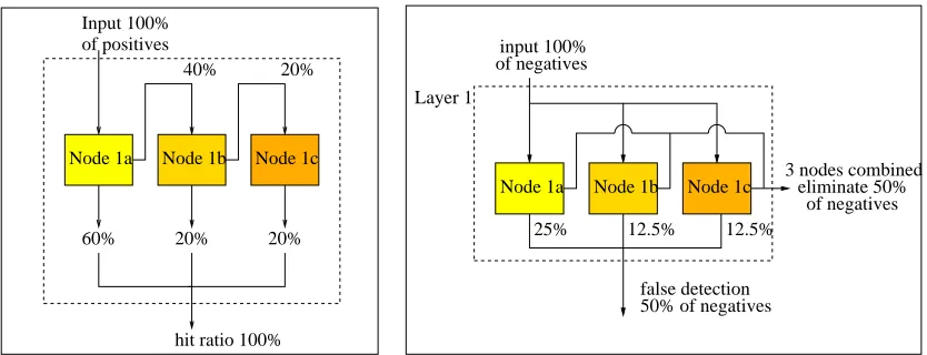
Whereas the cascading of the Viola-Jones method focuses on rejecting negative training samples which are then removed from the learning process, the intra-layer cascading of the PSL framework focuses on correctly predicting positive samples which are then removed from the intra-layer cascade of nodes. Thus, the underlying principle found in the Viola-Jones method with respect to its approach to handling more difficult negative samples with each succeeding layer, is applied to the positive samples in the node-to-node propagation of the PSL framework seen in Figure 2a. As the intra-layer cascade of nodes is constructed, correctly predicted positive samples are removed from succeeding nodes while the misclassified positives are retained until all the positive samples have been correctly predicted.

The mode of node-to-node propagation of the negative training samples in the intra-layer cascade is identical to the manner in which the positive training samples propagate from layer-to-layer in the Viola-Jones cascades. This means that all negative training samples are made available to each node irrespective of how successfully previous nodes have learned to predict them demonstrated in Figure 2b. Each node is assigned a target to learn to reject 50% of the negative samples and to achieve a 100% hit rate as in the Viola-Jones method. However a key constraint is added to each node which accelerates the layer convergence. This constraint restricts the size of each node to a predetermined maximum number of weak classifiers.

60%

40% 20%

20% 20%

hit ratio 100% Input 100%

of positives

Node 1a Node 1b Node 1c

50% of negatives false detection Layer 1

Node 1a Node 1b Node 1c

of negatives 12.5% 12.5%

25% of negativesinput 100%

eliminate 50% 3 nodes combined

Figure 2: a) The propagation of positive training samples within the cascade of PSL nodes inside a layer. 1 b) The usage of negative training samples within the cascade of PSL nodes inside a layer.

the layer false acceptance rates without an explicit guarantee of being secured. However, even if the false acceptance rates are found to be too high during training, the PSL structure has the capability to dynamically increase the maximum size of the nodes in order to meet targets.

The PSL framework addresses the inherent difficulty of CoBEs and accelerates the training runtimes by providing a solution to the slow convergence rates of cascade layer training by elimi-nating the trade-off between the primary layer target parameters. It also accelerates training due to the fact that it makes the computation of artificial layer adjustments redundant and guarantees each succeeding node will have to learn to predict a decreasing number of positive samples.

3

Method

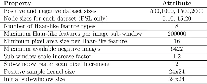
Experiments were devised to compare the PSL framework against the standard Viola-Jones frame-work. For both frameworks, four classifiers were trained; one classifier for each dataset of a different size whose properties are shown in Table 1. Additionally, the experiments sought to compare PSL classifiers produced with variations in the size of the nodes. Four node sizes were selected ranging from 5-20 weak classifiers at a 5 weak classifier increments. Each PSL node size produced four classifiers for each of the different training dataset sizes. Table 2 shows the training parameters used for producing these classifiers. The training data used for all classifiers was a subset of the FERET face dataset.

Table 1: Training settings and dataset details.

Property Attribute

Positive and negative dataset sizes 500,1000, 1500,2000 Node sizes for each dataset (PSL only) 5,10, 15,20

Number of Haar-like feature types 8

Maximum Haar-like features per image sub-window 200000 Minimum pixel area size per Haar-like feature 16

Maximum available negative images 6422

Sub-window scale increase factor 1.2

Sub-window raster scan pixel increment 2

Positive sample kernel size 24x24

Initial sub-window size 24x24

Table 2: Classifier tuning parameters for all experiments.

Property Setting

Target training error 0%

Target layer hit rate 100%

Target layer false alarm rate 50%

Maximum nodes per layer (PSL only) 10

Maximum layers 100

were 72,654,174. Each image was scanned by raster beginning with a 24x24 pixel kernel. After each calculation of a sub-window, the kernel shifted by two pixels until the entire image was scanned and thereafter increased by scale of 1.2. An error margin was given for each positive sample and calculated to be one quarter of image’s length and hight in each direction on its axis.

4

Results

The analysis of the results will focus on three areas. The first will compare the training phases of all classifiers. The second area will examine the accuracy of the classifiers while the third will present runtime performances. The goal of this section will be twofold. Firstly, we will attempt to draw conclusions from observations of how PSL classifiers trained with different node sizes have performed against one another in order to be able to ascertain what might be optimal node sizes for PSL training. Secondly, we will discuss the results of PSL classifiers in respect to those of Viola-Jones.

4.1

The Training Phase

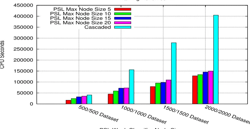
A zero training error rate was attained by all classifiers. The training runtimes comparing PSL classifiers of variable node sizes is shown in Figure 3. The figure shows that on this dataset, the classifiers with smaller nodes consistently produce training runtimes that are of a shorter duration. When comparing the PSL training runtimes to those of the Viola-Jones styled classifiers in the same figure, the difference becomes more pronounced. Here we see that the PSL classifiers are significantly faster at producing classifiers than the Viola-Jones method.

PSL structure increases the difficulty of satisfying the layer false acceptance rates. It also shows that succeeding nodes have the tendency to introduce a false acceptance rate in training that is in many cases considerably higher than that of the prior nodes, even if the prior nodes manage to achieve low false acceptance rates. This characteristic ultimately affects the potential training runtime since newer bootstrapped negative training samples will be introduced at a slower rate with each succeeding layer. The result is that an increased number of negative training samples from previous layers will be re-trained without improving the potential generalisation rate of a final classifier.

0 50000 100000 150000 200000 250000 300000 350000 400000 450000

500/500 Dataset 1000/1000 Dataset1500/1500 Dataset2000/2000 Dataset

CPU Seconds

PSL Weak Classifier Node Sizes Training Runtimes

PSL Max Node Size 5 PSL Max Node Size 10 PSL Max Node Size 15 PSL Max Node Size 20 Cascaded

Figure 3: Training runtimes in CPU seconds for all classifiers on the four CMU MIT datasets.

4.2

Classifier Accuracy

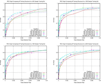
We use the receiver operating curves (ROC) to analyse classifier accuracy which is the standard measurement tool for classifiers. Figure 6 show classifiers for each of the training structures on four different datasets. They show only a selected and more relevant interval of the ROC curve for false detection rates of up to 0.01%. A consistent feature is found when comparing the PSL classifiers with varying node sizes. On this test dataset, the PSL classifiers trained with the smallest allowable node dimension produced the poorest generalisation rates on all datasets. As node sizes increase, there is clear evidence of partiality towards stronger generalisation rates. However, classifiers trained with the largest nodes did not exhibit superior generalisation on every dataset. These results do not permit a conclusion to be made on what is an optimal node dimension for training face detection PSL classifiers on datasets of any size but they do signify that a node size of below 10 weak classifiers is likely to compromise generalisation.

0 0.1 0.2 0.3 0.4 0.5 0.6

0 2 4 6 8 10

False alarm rate

Number of weak classifiers per layer Typical PSL False Alarm Rate Convergence - Layer 1

Cascade Layers Node 1 Node 2 0 0.1 0.2 0.3 0.4 0.5 0.6

0 2 4 6 8 10

False alarm rate

Number of weak classifiers per layer Typical PSL False Alarm Rate Convergence - Layer 2

Cascade Layers Node 1 Node 2 0 0.1 0.2 0.3 0.4 0.5 0.6

0 2 4 6 8 10

False alarm rate

Number of weak classifiers per layer Typical PSL False Alarm Rate Convergence - Layer 3

Cascade Layers Node 1 Node 2 0 0.1 0.2 0.3 0.4 0.5 0.6

0 2 4 6 8 10

False alarm rate

Number of weak classifiers per layer Typical PSL False Alarm Rate Convergence - Layer 4

Cascade Layers Node 1 Node 2 0 0.1 0.2 0.3 0.4 0.5 0.6

0 2 4 6 8 10

False alarm rate

Number of weak classifiers per layer Typical PSL False Alarm Rate Convergence - Layer 5

Cascade Layers Node 1 Node 2 0 0.1 0.2 0.3 0.4 0.5 0.6

0 2 4 6 8 10

False alarm rate

Number of weak classifiers per layer Typical PSL False Alarm Rate Convergence - Layer 6

Cascade Layers Node 1 Node 2 0 0.1 0.2 0.3 0.4 0.5 0.6

0 2 4 6 8 10

False alarm rate

Number of weak classifiers per layer Typical PSL False Alarm Rate Convergence - Layer 7

Cascade Layers Node 1 Node 2 0 0.1 0.2 0.3 0.4 0.5 0.6

0 2 4 6 8 10

False alarm rate

Number of weak classifiers per layer Typical PSL False Alarm Rate Convergence - Layer 8

Cascade Layers Node 1 Node 2

0 0.1 0.2 0.3 0.4 0.5 0.6

0 2 4 6 8 10

False alarm rate

Number of weak classifiers per layer Typical PSL False Alarm Rate Convergence - Layer 9

Cascade Layers Node 1 Node 2 0 0.1 0.2 0.3 0.4 0.5 0.6

0 2 4 6 8 10

False alarm rate

Number of weak classifiers per layer Typical PSL False Alarm Rate Convergence - Layer 10

Cascade Layers Node 1 Node 2 0 0.1 0.2 0.3 0.4 0.5 0.6

0 2 4 6 8 10

False alarm rate

Number of weak classifiers per layer Typical PSL False Alarm Rate Convergence - Layer 11

Cascade Layers Node 1 Node 2 0 0.1 0.2 0.3 0.4 0.5 0.6

0 2 4 6 8 10

False alarm rate

Number of weak classifiers per layer Typical PSL False Alarm Rate Convergence - Layer 12

Cascade Layers Node 1 Node 2 0 0.1 0.2 0.3 0.4 0.5 0.6

0 2 4 6 8 10

False alarm rate

Number of weak classifiers per layer Typical PSL False Alarm Rate Convergence - Layer 13

Cascade Layers Node 1 Node 2 0 0.1 0.2 0.3 0.4 0.5 0.6

0 2 4 6 8 10

False alarm rate

Number of weak classifiers per layer Typical PSL False Alarm Rate Convergence - Layer 14

Cascade Layers Node 14 Node 2 0 0.1 0.2 0.3 0.4 0.5 0.6

0 2 4 6 8 10

False alarm rate

Number of weak classifiers per layer Typical PSL False Alarm Rate Convergence - Layer 15

Cascade Layers Node 1 Node 2 Node 3 0 0.1 0.2 0.3 0.4 0.5 0.6

0 2 4 6 8 10

False alarm rate

Number of weak classifiers per layer Typical PSL False Alarm Rate Convergence - Layer 16

Cascade Layers Node 1 Node 2

The elevated false detection rate of the PSL framework is a consequence of a flaw in the training structure’s current approach to training nodes in each layer. At present, we observe that the first node in each layer is exposed to all positive samples from a training dataset while the succeeding nodes ’see’ subsets of the original with ever decreasing sizes. It is often the case that the final nodes in a layer are exposed to very few positive samples resulting in overfitting. Since at detection time a negative sample can only be rejected if all nodes in a layer correctly predict the sample as a negative, the false detection rate for any given layer will only be as good as the performance of its weakest node. Thus a chain is only as strong as its weakest link. When the entire cascade is considered in the PSL framework, the overall false detection becomes the combined accuracy of the weakest nodes from each layer.

0.5 0.6 0.7 0.8 0.9 1

0 0.002 0.004 0.006 0.008 0.01

Hit Rate

False Detection Rate

ROC Graph Comparing All Training Structures for a 500 Sample Training Set

Classifiers: PSL with Node Size 5 PSL with Node Size 10 PSL with Node Size 15 PSL with Node Size 20 Cascaded with Threshold

0.5 0.6 0.7 0.8 0.9 1

0 0.002 0.004 0.006 0.008 0.01

Hit Rate

False Detection Rate

ROC Graph Comparing All Training Structures for a 1000 Sample Training Set

Classifiers: PSL with Node Size 5 PSL with Node Size 10 PSL with Node Size 15 PSL with Node Size 20 Cascaded with Threshold

0.5 0.6 0.7 0.8 0.9 1

0 0.002 0.004 0.006 0.008 0.01

Hit Rate

False Detection Rate

ROC Graph Comparing All Training Structures for a 1500 Sample Training Set

Classifiers: PSL with Node Size 5 PSL with Node Size 10 PSL with Node Size 15 PSL with Node Size 20 Cascaded with Threshold

0.5 0.6 0.7 0.8 0.9 1

0 0.002 0.004 0.006 0.008 0.01

Hit Rate

False Detection Rate

ROC Graph Comparing All Training Structures for a 2000 Sample Training Set

Classifiers: PSL with Node Size 5 PSL with Node Size 10 PSL with Node Size 15 PSL with Node Size 20 Cascaded with Threshold

Figure 6: ROC graph curves for on the CMU MIT datasets showing the generalisation patterns of all classifiers. a) 500 positive/500 negative CMU MIT dataset. b) 1000 positive/1000 negative CMU MIT dataset. c) 1500 positive/1500 negative CMU MIT dataset. d) 2000 positive/2000 negative CMU MIT dataset.

4.3

The Detection Phase Performance

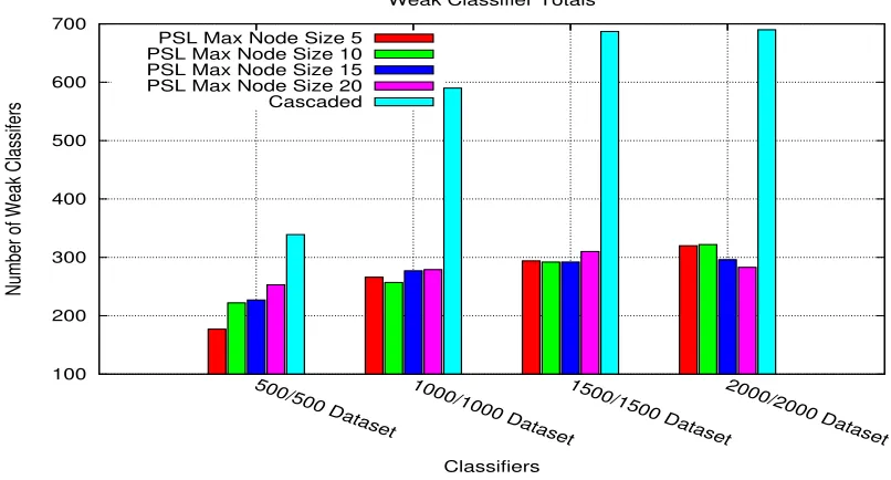
when comparing the PSL and Viola-Jones methods, the largest classifiers were created by the Viola-Jones framework. The PSL classifiers consisted of a fraction of the size of the Viola-Jones classifiers.

100 200 300 400 500 600 700

500/500 Dataset 1000/1000 Dataset1500/1500 Dataset2000/2000 Dataset

Number of Weak Classifers

Classifiers Weak Classifier Totals

PSL Max Node Size 5 PSL Max Node Size 10 PSL Max Node Size 15 PSL Max Node Size 20 Cascaded

Figure 7: Weak classifiers totals per strong classifiers for each framework on the four CMU MIT datasets.

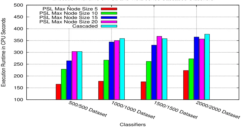
The correlation between the number of weak classifiers generated by the learning framework and its execution runtime can be seen in Figure 8. The figure provides classifier runtime perfor-mances on the test dataset showing that the PSL classifiers outperform the Viola-Jones classifiers. However, the figure also shows that as the node sizes for the PSL classifiers increase, their runtime performance begins to resemble that of the Viola-Jones classifiers.

PSL Discussion

A better understanding has been gained regarding the role intra-layer node sizes defined at training, influence the accuracy and the performances of the resulting classifiers. The training runtimes are fastest for classifiers constructed with smallest node sizes and increase as the size of the nodes is enlarged. Likewise, execution runtimes are most rapid for classifiers trained with smaller nodes and continue to rise with increases in node sizes.

The analysis of PSL classifier accuracy has shown that there does not exist an exact linear improvement with increases or decreases in node sizes. In this problem domain and test dataset, classifiers with larger nodes have for the most part shown a better generalisation pattern but based on the results it is not possible to say exactly which one node size is the most suitable for producing optimal classifiers on datasets of varying sample sizes. The issue of setting optimal node sizes for training PSL classifiers appears domain specific and depends on the difficulty of the target object being trained.

100 150 200 250 300 350 400 450 500

500/500 Dataset 1000/1000 Dataset1500/1500 Dataset2000/2000 Dataset

Execution Runtime in CPU Seconds

Classifiers

Execution Runtime of PSL and Viola-Jones Cascaded Classifers

PSL Max Node Size 5 PSL Max Node Size 10 PSL Max Node Size 15 PSL Max Node Size 20 Cascaded

Figure 8: Execution runtimes for PSL and Viola-Jones classifiers on the CMU MIT test datasets.

guarantees that a minimal number of positives samples are present in the final node in order to prevent over-training occuring on a handful of positive samples.

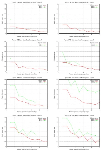
The difficulty of achieving layer targets as node numbers increase has also been highlighted. Figures 4 and 5 have shown the pattern of convergence of the false acceptance rates which is obstructed in the PSL framework for two reasons. The first reason can be seen in these figures at the conclusion of the creation of each node. All previous information regarding the performance of the negative training samples is lost since the AdaBoost algorithm resets all sample weights and the boosting process re-starts from the beginning. [20] point out that this is valuable information which can assist in producing faster convergence rates in succeeding layers and they show how this information can be recycled through the idea of soft-cascades. Even though their suggestions refered only to inter-layer cascading of Viola-Jones instead of intra-layer cascading occuring in PSL, some ideas can be applied here.

The second reason is that the learning algorithm does not have the ability to differentiate between negative samples which have been misclassified by previous nodes and those that have not. The consequence is that AdaBoost inevitably focuses on rejecting negative samples in a given node which cannot be ultimately rejected by the cascade-of-nodes as a whole. This is the case since a unanimous vote is necessary by all the nodes in a layer, thus finally eroding the layer false acceptance rates. One possible possible solution that would allow AdaBoost to focus only on specific negative samples would be to propagate from node to node only those negative samples which have been correctly predicted by the previous nodes in a layer.

5

Conclusion

in comparison to the Viola-Jones method.

A deeper understanding into the PSL structure has been gained in respect to the setting of parameters for its unique intra-layer cascading component. The experiments show that by decreasing the maximum allowable number of weak classifiers per intra-layer cascade, there arises a clear and general reduction in training as well as execution runtimes. However, the optimal setting of this particular parameter on accuracy has been revealed to be application domain specific.

Future work on the PSL framework will involve efforts to address the problem of increased false acceptance rates which play a more critical role in application domains operating under the rare-event detection constraints.

References

[1] Barczak, A.L.C., Johnson, M.J., Messom, C.H.: Empirical evaluation of a new structure for adaboost. In: SAC ’08: Proceedings of the 2008 ACM symposium on Applied computing, Fortaleza, Ceara, Brazil, ACM (2008) 1764 – 1765

[2] Brubaker, S.C., Mullin, M.D., Rehg, J.M.: Towards optimal training of cascaded detectors. Proc. of Computer Vision. ECCV 20063951(2006) 325–337

[3] Pham, M.T., Cham, T.J.: Fast training and selection of haar features using statistics in boosting-based face detection. Computer Vision, 2007. ICCV 2007. IEEE 11th International Conference on (Oct. 2007) 1–7

[4] Wu, J., Rehg, J.M., Mullin, M.D.: Learning a rare event detection cascade by direct feature selection. In: NIPS (Advances in Neural Information Processing Systems) 2003, Vancouver, Canada (2003)

[5] Baluja, S., Sahami, M., Rowley, H.: Efficient face orientation discrimination. In: Proc. International Conference on Image Processing ICIP’04. Volume 1. (2004) 589–592 Vol. 1 [6] Wu, Jianxin; Brubaker, S.C.M.M.D.R.J.M.: Fast asymmetric learning for cascade face

de-tection. IEEE Transactions on Pattern Analysis and Machine Intelligence 30 (2008) 369 – 382

[7] Viola, P., Jones, M.: Robust real time object detection. In: SCTV01. (2001) xx–yy

[8] Mita, T., Kaneko, T., Hori, O.: Joint haar-like features for face detection. In: 10th IEEE International Conference in Computer Vision (ICCV’05), IEEE (2005) 1619–1626

[9] Xiao, R., Zhu, L., Zhang, H.J.: Boosting chain learning for object detection. In: ICCV ’03: Proceedings of the Ninth IEEE International Conference on Computer Vision, Washington, DC, USA, IEEE Computer Society (2003) 709

[10] Withopf, D., Withopf, D., Jahne, B.: Improved training algorithm for tree-like classifiers and its application to vehicle detection. In Jahne, B., ed.: Proc. IEEE Intelligent Transportation Systems Conference ITSC 2007. (2007) 642 – 647

[11] Lienhart, R., Maydt, J.: An extended set of haar-like features for rapid object detection. In: ICIP02, Rochester, NY (September 2002) I: 900–903

[12] Friedman, J., Hastie, T., Tibshirani, R.: Additive logistic regression: a statistical view of boosting. Annals of Statistics28(2000) 2000

[14] Viola, P.A., Jones, M.J.: Fast and robust classification using asymmetric adaboost and a detector cascade. In Dietterich, T.G., Becker, S., Ghahramani, Z., eds.: NIPS. (2001) 1311– 1318

[15] Luo, H.: Optimization design of cascaded classifiers. Computer Vision and Pattern Recogni-tion, 2005. CVPR 2005. IEEE Computer Society Conference on1 (June 2005) 480–485 vol. 1

[16] Brubaker, S.C., Wu, J., Sun, J., Mullin, M.D., Rehg, J.M.: On the design of cascades of boosted ensembles for face detection. Int. J. Comput. Vision77(1-3) (2008) 65–86

[17] Susnjak, T., Barczak, A.: Accelerated Classifier Training Using the PSL Cascading Structure. (2009)

[18] Susnjak, T.: Accelerating classifier training using AdaBoost within cascades of boosted en-sembles: a thesis presented in partial fulfillment of the requirements for the degree of Master of Science in Computer Sciences at Massey University, Auckland, New Zealand. Master’s thesis (2009)

[19] Sung, K., Poggio, T.: Example-based learning for view-based face detection. IEEE Patt. Anal. Mach. Intell.20(39-51) (1998)