City, University of London Institutional Repository
Citation
:
Cavaglià, A. (2015). Nonsemilinear one-dimensional PDEs: analysis of PT deformed models and numerical study of compactons. (Doctoral thesis, City University London)This is the accepted version of the paper.
This version of the publication may differ from the final published
version.
Permanent repository link: http://openaccess.city.ac.uk/13074/
Link to published version
:
Copyright and reuse:
City Research Online aims to make research
outputs of City, University of London available to a wider audience.
Copyright and Moral Rights remain with the author(s) and/or copyright
holders. URLs from City Research Online may be freely distributed and
linked to.
City Research Online: http://openaccess.city.ac.uk/ [email protected]
PDEs: analysis of
PT
deformed
models and numerical study of
compactons
Andrea Cavagli`a
Department of Mathematics
School of Mathematics, Computer Science and Engineering
City University London
A thesis submitted for the degree of
Doctor of Philosophy in Mathematical Physics
This thesis is based on the work done during my PhD studies and is roughly divided in two independent parts. The first part consists of Chapters 1 and 2 and is based on the two papers Cavagli`aet al.[2011] and Cavagli`a & Fring [2012], concerning the complex PT-symmetric deformations of the KdV equation and of the inviscid Burgers equa-tion, respectively. The second part of the thesis, comprising Chapters 3 and 4, contains a review and original numerical studies on the prop-erties of certain quasilinear dispersive PDEs in one dimension with compacton solutions.
The subjects treated in the two parts of this work are quite different, however a common theme, emphasised in the title of the thesis, is the occurrence of nonsemilinear PDEs. Such equations are charac-terised by the fact that the highest derivative enters the equation in a nonlinear fashion, and arise in the modeling of strongly nonlinear natural phenomena such as the breaking of waves, the formation of shocks and crests or the creation of liquid drops. Typically, nonsemi-linear equations are associated to the development of singularities and non-analytic solutions.
Many of the complex deformations considered in the first two chapters are nonsemilinear as a result of the PT deformation. This is also a
crucial feature of the compacton-supporting equations considered in the second part of this work.
This thesis is organized as follows.
ily of complex models obtained as PT-symmetric deformations of the KdV equation. We also illustrate with many examples the connec-tion between the periodicity of orbits and their invariance under PT
-symmetry.
Chapter 2 is based on the paper Cavagli`a & Fring [2012] on thePT -symmetric deformation of the inviscid Burgers equation introduced in Bender & Feinberg [2008]. The main original contribution of this chapter is to characterise precisely how the deformation affects the gradient catastrophe. We also point out some incorrect conclusions of the paper Bender & Feinberg [2008].
Chapter 3 contains a review on the properties of nonsemilinear dispersive PDEs in one space dimension, concentrating on the com-pacton solutions discovered in Rosenau & Hyman [1993]. After an in-troduction, we present some original numerical studies on the K(2,2) and K(4,4) equations. The emphasis is on illustrating the different type of phenomena exhibited by the solutions to these models. These numerical experiments confirm previous results on the properties of compacton-compacton collisions. Besides, we make some original ob-servations, showing the development of a singularity in an initially smooth solution.
Contents vi
List of Figures ix
1 PT -symmetric deformations of nonlinear wave equations 1
1.1 Complex extensions of dynamical systems . . . 1
1.2 A brief introduction toPT-symmetric quantum mechanics . . . . 2
1.2.1 Physical applications . . . 5
1.2.2 Comparison of quantum/classical behaviour . . . 6
1.2.3 PT symmetric deformations of nonlinear wave equations . 8 1.3 The KdV equation: complex extension of travelling waves and PT-symmetric deformations . . . 9
1.3.1 The KdV equation and its PT-symmetric deformations . 9 1.3.2 Complex extension of travelling waves . . . 13
1.3.3 The undeformed equation . . . 16
1.3.3.1 Rational solutions . . . 16
1.3.3.2 Trigonometric solutions . . . 17
1.3.3.3 Elliptic solutions . . . 23
1.3.4 Deformations of the KdV equation I: the PT+-symmetric deformation . . . 26
1.3.4.1 Rational solutions . . . 29
1.3.4.2 Trigonometric solutions . . . 31
1.3.4.3 Elliptic solutions . . . 35
1.3.5.1 An example with ǫ= 4 . . . 37
1.4 Complex deformations of soliton solutions . . . 39
1.5 Summary of the results of this chapter . . . 41
2 PT -symmetric deformation of the inviscid Burgers equation 43 2.1 The undeformed case . . . 44
2.1.1 Inviscid Burgers equation, characteristics and gradient catas-trophe . . . 44
2.1.2 Singularities as branch points . . . 45
2.1.3 Shocks and weak solutions . . . 48
2.2 Deformed case (ǫ >1) . . . 49
2.2.1 Singularities . . . 50
2.3 Summary of the results of this chapter . . . 60
3 Numerical study of the Rosenau-Hyman compacton equations 61 3.1 Solutions with compact support in degenerate equations . . . 62
3.2 The porous medium equation . . . 63
3.2.0.1 Heuristic derivation of the edge equation . . . . 66
3.3 The equations of Rosenau and Hyman and compactons . . . 68
3.3.1 Compacton solutions . . . 69
3.3.1.1 Compactons as weak solutions . . . 70
3.3.2 Interactions of compactons . . . 73
3.3.2.1 Other general properties . . . 75
3.4 Numerical study of the K(2,2) and K(4,4) equations . . . 77
3.4.1 General description of the numerical method . . . 78
3.4.2 Numerical experiments: the K(2,2) equation . . . 80
3.4.3 Numerical experiments: the K(4,4) equation . . . 89
3.5 Summary of the results of this chapter . . . 94
4 Numerical study of stability for an integrable compacton equa-tion 97 4.1 Integrable quasi-linear equations, hodograph transformations and the Lagrange map . . . 98
4.2.1 Special solutions . . . 105
4.2.2 A heuristic argument for the instability of travelling com-pactons . . . 108
4.2.2.1 A family of deformations . . . 109
4.2.3 Conservation laws and behaviour at the edge of the support 111 4.3 Numerical study . . . 116
4.3.1 Decomposition of positive initial data . . . 117
4.3.2 Comparison with other equations with δ 6= 0 . . . 121
4.4 Summary of the results of this chapter . . . 123
5 Conclusions 126 A Classification of two-dimensional stationary points 129 B Details on the numerical schemes used to integrate compacton equations 131 C Study of the compactly-supported travelling solutions of the equations (4.27) 135 C.1 Case v >0 . . . 136
C.2 Case v <0 . . . 140
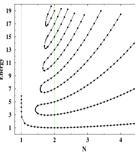
1.1 The first excited energy levels of the Hamiltonians (1.2) as a func-tion of the deformafunc-tion parameter, where N :=ǫ+ 2. The plot is taken from Bender & Boettcher [1998]. . . 3 1.2 Complex rational solutions of the KdV equation: in the left panel
PT-symmetric solutions for c = 1, β = 2, γ = 3 and A = 1/2;
in the right panel, we have taken c = 1, β = 2 +i2, γ = 3 and consequently A= (1−i)/4. . . 17 1.3 Left panel: PT+-symmetric solitary wave solutions of the KdV
equation with c = 1, β = 3/10, γ = −3, A = 4 and B = 2. Right panel: complex periodic PT+-symmetric solutions of the KdV equation with c = 1, β = 3/10, γ = 3, A = 4, B = 2. The period isT = 2√15π. . . 20 1.4 Complex trigonometric solutions of the KdV equation with
“spon-taneously broken” PT-symmetry. c = 1, β = 3/10, γ = 3,
A = 4 +i/2 and B = 2−i, meaning that this family of orbits break the PT+-symmetry of the equation. All orbits of this type
are in the present case open. . . 21 1.5 Detail of a trigonometric solution of the complexified KdV equation
with broken PT-symmetry. Here we have taken c= 1, β = 3/10,
1.6 Two solutions of the non PT-symmetric complex KdV equation, where the parameters have been finely tuned in order to obtain a solitary wave solution (left panel), or a periodic solution (right panel). The choice of parameters is: Left: c= 1,β = (16−4i)/17,
γ =−3,A= 4+i,B =−5−5/4i; Right: c= 1,β = (−8+2i)/17,
γ =−3 and A= 4 +i,B =−14−7/2i . . . 23 1.7 PT-symmetric complex elliptic solutions of the KdV equation with
A= 1, B = 3, C = 6, c= 1, β = 3/10, γ =−3 for different values of Imζ0. . . 24
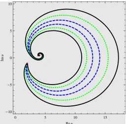
1.8 Spontaneously broken PT-symmetric complex elliptic solution of the KdV equation for Imζ0 = 6 with A = 4, B = 5−i/2, C =
1 +i/2, c = 1, β = 3/10 and γ = 3. The left panel shows the trajectory for −64≤ ζ ≤ 18 solid (red) and 18 < ζ ≤ 200 dashed (black). In the right panel: −200 < ζ < 1400. Notice that this is a single, space-filling trajectory. . . 25 1.9 BrokenPT-symmetric complex elliptic solutions of the KdV
equa-tion for Imζ0 = 6: in the left panel, A = 1, B = 3, C = 6, c= 1,
β = 3/10 and γ = 3 + 2i for −200 ≤ ζ ≤ 200; in the right panel,
A = 1, B = 2 + 3i, C = 6, c= 1, β = 3/10−i/10 and γ = 3 for
−200≤ζ ≤200. . . 26 1.10 Complex PT-symmetric rational solutions of the deformed KdV
equation with c = 1, β = 2 and γ = 3 for the deformed model
H+
−1/2, corresponding to the behaviour (1.54) with k = 1/2 and
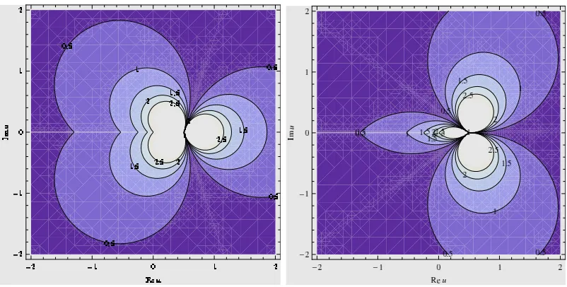
α= 6. . . 28 1.11 Complex PT-symmetric rational solutions of the deformed KdV
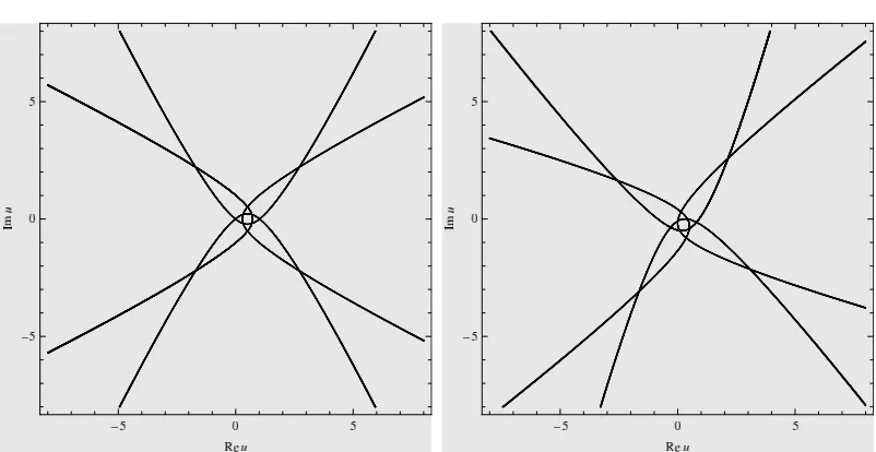
1.12 Contour plot showing differentPT-symmetric rational solutions of the H+1/3 equation, with c= 1, β = 2 andγ = 3, corresponding to equation (1.54) with k = 1/2 and α = 9/4. The system is defined on a four-sheet covering of the complex u-plane: in the left and right panel, we show the shape of orbits on the first two sheets. On the remaining two sheets, the picture would be the same, with the orbits being travelled in the opposite direction. . . 30 1.13 In the left panel are shown four different orbits (all of them
char-acterised by Im(ζ0) = 1) of the H+6 model with c= 1, β = 2 and
γ = 3, corresponding to (1.54) with k = 1/2 and α = 3/7. Each orbit makes a turn around the point u=A and is deflected by an angle which approaches asymptotically 74π. Notice that these four orbits live on different Riemann sheets, so that the are no intersec-tions. In the right panel, we break PT-symmetry by takingc= 1,
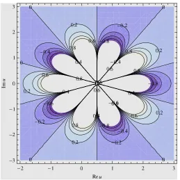
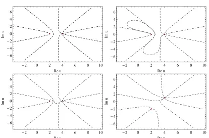
β = 2 + 2i and γ = 3, leading to k = 1/4(1−i), and the same value ofα. Clearly this simply amount to a rotation. . . 31 1.14 The network of separatrix curves for different solutions of theH+
−1 2
model for c = 1, β = 3/10, γ = 3. The critical points A and B
are chosen as: (top left) A= 4, B = 2 ; (top right):A= 4 + i 200000,
B = 2− 100000i ; (bottom left): A = 4 + 50i , B = 2− 25i ; (bottom right): A = 4 + i, B = 2− 2i . Notice that the topology of the network corresponding to the first solution (the PT-symmetric case) differs from the other three and does not allow the existence of orbits connecting A and B. . . 33 1.15 Complex PT-symmetric trigonometric/hyperbolic solutions of the
deformed KdV equation with A = 4, B = 2, c = 1, β = 2 and
γ = 3 for H+
−1/2. . . 34
1.16 Trigonometric/hyperbolic solutions of the deformed KdV equation
H+
−1/2 with spontaneously broken PT-symmetry. The relevant
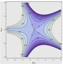
1.17 Complex PT-symmetric trigonometric/hyperbolic solutions of the
H+−2 deformation with c = 1, β = 2 and γ = 3. In the left panel, the solution is symmetric with A = 4, B = 2. In the right panel, it is spontaneously broken, with A= 4 +i/2, B = 2−i. . . 35 1.18 PT-symmetric solutions for H−4 : (a) Star node at the origin for
c = 1, β = 2, γ = 1; (b) centre at the origin for c = 1, β = 1,
γ = −1. In both cases there are four turning points at u = ±B,
±iB, with B = (15/2)1/4 . . . . 37
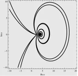
1.19 Broken PT-symmetry for the H−4 model: these solutions spiral around a focus at u = 0, accompanied by four turning points at
u =±B, ±iB, with B = (15/2)1/4 . The parameters were chosen
as c= 1, β = 2, γ = 1 +i3. . . 38 1.20 Complex spontaneously broken one-soliton solution of the
KdV-equation with β= 6, γ = 1 +i/2,p1 = 2, φ =i0.8 and ∆t=−π/2
for different times t = −π/2 solid (blue), t = −1 dashed (red),
t = 0 dasheddot (orange), t = 0.7 dotted (green), and t = π/2 dasheddotdot (black). . . 40 1.21 PT-symmetric two-soliton solutions of the KdV equation forβ = 6,
γ = 1, p1 = 1.2, p2 = 2.2, φ1 = i0.1 and φ2 = i0.2. Left panel:
t=−2 solid (blue), t=−0.2 dashed (red), t= 0.2 dotted (black); right panel: t = 0.3 dotted (black), t = 0.8 dashed (red), t = 2.0 solid (blue). . . 41 1.22 Broken PT-symmetric two-soliton solutions of the KdV equation
for β = 6, γ = 1 +iπ/8, p = 2(2/3)1/3, p
2 = 2, φ1 = i0.1 and
φ2 =i0.2. Left panel: t=−4 solid (blue), t=−3.5 dashed (red),
t = −2. dotted (black); right panel: t = 0.7 solid (blue), t = 2 dashed (red), t = 8 dotted (black). Notice that for this choice of parameters we have 2∆1
t = 3∆2t = 6. We see that both solitons
have almost regained their original shape passing from t = 2 to
2.1 Snapshots of the solution w(x, t) to the inviscid Burgers equation with initial condition w(x,0) = 1+x1 2. The solid lines correspond
to t= 0, t= 0.8 and t=ts = 3√83 ≃1.5396 (the crest of the wave
moves rightwards for increasing times). The dotted multi-valued profile corresponds tot =ts+ 1. . . 46
2.2 Trajectories traced in the complex x-plane by the square root branch points of the solution of (2.1) with initial conditionw(x,0) =
1
1+x2. There are four distinct trajectories, all traced fort in the
in-terval t∈[0.0001,1.75]. We observe that two singularities emerge from each of the two poles x = ±i at t = 0+. One pair of
com-plex conjugate singularities moves off in the in the comcom-plex plane, while the other two singularities reach the real axis simultaneously att =ts= 3√83. They remain confined to the real axis for t > ts. 47
2.3 In the left panel, trajectories traced in the complexx-plane by the square-root branch points of the ǫ= 2 solution with u0(x) = 1+x1 2.
In the right panel, we consider the ǫ = 2.2 deformation with the same initial condition (in this case, we are showing only some of the singularities, the ones corresponding to the principal branch in the definition ofW0(ǫ)). In both plots the trajectories are shown for t ∈[10−6,0.36]; the arrow of time is such that the square-root
branch points move out of the poles at x=±i ast increases from
t= 0+. . . . . 52
2.4 Trajectories of square root branch points in the complex x-plane, for the ǫ = 3 (left) and ǫ = 5 deformation (right), where the initial condition was chosen again as u0(x) = 1+x1 2. In both plots
the trajectories correspond to t ∈[10−6,0.4], and move out of the
2.5 Left panel: space-time plot of (2.1) with initial condition w0(x) =
W0(3)(x) defined by (2.17) with ǫ= 3, u0(x) = 1+x1 2, for 0< t < ts
Right panel: the corresponding solution of the ǫ = 3-deformed model, in the same time interval. One can see that, as t → t−
s,
w(ǫ)x → ∞, while foru this appears as uxx → ∞. . . 54
2.6 Left: solution of the ǫ= 2-deformed inviscid Burgers equation for
u0(x) = 1+x1 2 at timest= 0 (blue, dashed),t= 0.1 (purple, dotted)
and at the singularity time t = ts ∼ 0.191 (red, solid). Right:
solution of the ǫ = 5/2-model with the same initial condition, shown for t = 0 (blue, dashed), t = 0.1 (purple, dotted) and
t =ts ∼0.176 (red, solid). The black dots mark the places where
uxx → ∞. . . 55
2.7 Left: solution of the ǫ = 3-model with u0(x) = 1+x1 2, shown for
t = 0 (blue, dashed), t = 0.1 (purple, dotted) and t =ts ∼ 0.312
(red, solid). Right: solution of the ǫ = 5-model with the same initial condition, shown for t = 0 (blue, dashed), t = 0.1 (purple, dotted) and t =ts ∼ 0.395 (red, solid). The black dots mark the
places where uxx → ∞. . . 55
2.8 Solution of the ǫ = 3 equation with u0(x) = 1+x1 2 at the time of
appearance of the second singularity t =ts,2 ∼ 0.64> ts,1 ∼0.31.
The vertical line marks the location xs,2 ∼ −1.2. Notice that,
around xs,1 ∼0.08, the solution has branched into a multi-valued
profile with a self-intersection. . . 57 2.9 These two figures illustrate the mechanism of formation of a
self-crossing profile in real solutions of the deformed equation after the breaking time. A multivalued profile of the undeformed equa-tion (left) is transformed into a self-intersecting profile for ˜u =
iuǫ−ǫ1(right) according to (2.28). The vertical line in the left plot
preserves the area shaded by the graph of ˜w = (w(ǫ)(x, t))ǫ−11.
It corresponds to a self-intersection for the graph of ˜u since 0 =
Rs2
s1 −
Rs3
s2 +
Rs4
s3
˜
2.10 Snapshots of the solution of the ǫ = 3 deformation with initial conditionu(x,0) = 1+xx2, shown at timet= 0 (red, dotted),t= 1.5
(blue, dashed) and t =tshock= 13 (solid, black). . . 59
3.1 The Barenblatt solution (3.7) of the porous medium equation with
m = 3, with the parameter choice β = 1, shown at times t = 1,
t = 2, t = 3, t = 4, t = 5. The support of the solution spreads as time increases. . . 64 3.2 The shapes of compacton solutions to the K(2,2) equation (blue,
dotted), to the K(3,3) equation (purple, dashed), and to the K(4,4) equation (black, solid). In all cases we took c= 1. The behaviour of these three solutions close to the endpoints e± of the support is
u2,2 ∼ |x−e±|2, u3,3 ∼ |x−e±|, and u4,4 ∼ |x−e±|
2
3, respectively. 71
3.3 Numerical solution of the K(2, 2) equation showing the scatter-ing among two compactons of speeds c1 = 1 and c2 = 3. This
simulation was performed with η2 = 0 andη4 = 10−3. . . 81
3.4 Detail of the ripple left by the collision of two compactons, for the same data shown in Figure 3.3. The compacton on the right of the picture is the c = 1 compacton after its emergence from the interaction. . . 82 3.5 K(2,2) equation: evolution of the initial conditionu(x,0) = cos4(x
6)χ[−3π,3π](x)
. The data in the plot were obtained by adding the viscosityη2 = 0
and η4 = 10−3. . . 84
3.6 K(2,2) equation: decomposition of very narrow initial datau(x,0) = cos4(3x
4 )χ[−23π, 2
3π](x), showing a sequence of shocks formed close to
the left endpoint of the support. The simulation was done with added dissipation η4 = 10−3. . . 85
3.7 Evolution of the same data as in Figure 3.6, for larger times. . . 85 3.8 Illustration of the steepening at the right edge of the support for
the same data as in Figure 3.5. . . 86 3.9 K(2,2) equation: evolution of the initial conditionu(x,0) = sin(πx3 )+
3.10 Detail of the approach to singularity for the same solution to the K(2,2) equation as in Figure 3.9. Dots (black) represent the nu-merical solution obtained without adding any dissipative term, while the continuous (light-blue) line was obtained withη4 = 10−3
(the two curves are almost indistinguishable in the plot). . . 89 3.11 K(4,4) equation: collision among two compactons with speedsc1 =
2 and c2 = 1. This simulation was obtained with added viscosity
η2 = 0 andη4 = 3×10⁻⁵. . . 90
3.12 The figure shows two later snapshots of the evolution of the same data as in Figure 3.11, showing the separation of the c = 1 com-pacton from the residual left at the site of the interaction (notice that the faster, c = 2 compacton has been removed and is not visible in the plot). . . 91 3.13 K(4,4) equation: decomposition of the compactly supported
ini-tial data u(x,0) = cos(πx20)χ[−10,10](x). Data obtained with added
dissipation η4 = 10−4. . . 92
3.14 Initial phase of the decomposition of the profileu(x,0) =u(x,0) = cos4(πx
20)χ[−10,10](x), showing in detail the spiky oscillations formed
close to the left edge of the support. As compared to the data in Figure 3.13, the oscillations are more pronounced, but appear to have the same shape. These data were obtained with η2 = 0 and
η4 = 10−4. . . 93
3.15 K(4,4) equation: evolution of the smooth positive profileu(x,0) = 1.1 + sin(πx10). It is shown how this profile approaches the line
u = 0 forming a number of singular spikes. Data obtained with
η2 =η4 = 0. . . 94
4.1 Numerical solution of the equation (4.10) with initial condition
u(x,0) = 1.1 + sin(π
3x). The solution approaches the line u = 0
forming spikes with the shape (4.15). . . 105 4.2 Snapshots of an asymptotically stationary two-compacton solution.
4.3 Decomposition of the initial conditionu(x,0) = cos(π4(x−2))χ[0,4](x).
The solution develops a moving interface expanding leftwards and approaches a stationary compacton solution (4.20) as t→ ∞. . . 118 4.4 Decomposition of the initial conditionu(x,0) = cos(π8(x−4))χ[0,8](x).
The solution appears to approach a train of two stationary com-pacton solutions for large times. . . 119 4.5 Space-time trajectories of the maximum of the solution (blue,
dot-ted line) and of the left edge point of the support (black, dashed line) for the solution represented in Figure 4.3. The trajectory traced by the edge point matches precisely the prediction of (4.50) (represented by red crosses). . . 120 4.6 Numerical solution of the integrable δ = 0 equation with initial
condition u(x,0) = 2 cos2((x−2)π
12)χ[−4,8](x). . . 121
4.7 Numerical solution of the deformed δ = 1/4 equation with ini-tial condition u(x,0) = 2 cos2((x−2)π
12)χ[−4,8](x). The structure
emerging on the right fits very well with the shape of a stationary compacton solution. . . 122 4.8 Numerical solution of the deformedδ = 3
4 equation with initial
con-ditionu(x,0) = 2 cos2((x−2)π
12)χ[−4,8](x). The structure emerging
from the right is a travelling compacton solution with speed ap-proximately c∼0.60. . . 123 C.1 Depiction of the orbits of equation (C.10) with c=−1, U >0 for
different values of δ. Left: δ= 1.5, Right: δ= 0. . . 138 C.2 The orbits of (C.10) with c = −1, U < 0, for different values of
PT
-symmetric deformations of
nonlinear wave equations
1.1
Complex extensions of dynamical systems
In this chapter we consider complex deformations of classical systems, motivated by the analogy with PT-symmetric quantum mechanics.
Complex extensions of classical systems have been considered in different con-texts, often revealing that crucial aspects of the dynamics of a real system can be best understood as images of simpler phenomena happening in a larger complex domain. For example, the connection between the integrability of a dynamical system and its analytic properties when extended to complex time, first discov-ered in the seminal work of Kovalevskaya Kowalevski [1889], is at the heart of the celebrated Painlev`e conjecture Ablowitzet al.[1978]. More recently, complex-time dynamical systems have been considered in the attempt to understand the fundamental mechanisms underlying chaos, see for example Calogeroet al.[2005]. From another perspective, a great interest in complex classical systems has also arisen in conjunction with the study PT-symmetric quantum mechanics
investigations gave rise to an independent field of research into the often surpris-ing properties of these models, even when considered purely at the classical level. This chapter is based on the work Cavagli`aet al. [2011], and deals with the study of complex travelling wave solutions to the KdV equations and itsPT-symmetric
deformations.
1.2
A brief introduction to
PT
-symmetric
quan-tum mechanics
The field of PT-symmetric quantum mechanics stems from the discovery that some quantum one-dimensional Hamiltonians, despite not being manifestly Her-mitian with respect to the standard L2(R) metric, may still admit a purely real
spectrum, bounded from below Bender & Boettcher [1998]. Bender and Boettcher quote as a main source of inspiration an unpublished work by Bessis and Zinn-Justin, who conjectured that the complex cubic oscillator
H1 =p2+i x3, (1.1)
relevant to describe the Yang-Lee edge singularity in statistical mechanics Fisher [1978], may have a real spectrum. Bender and Boettcher investigated numerically the family of complex anharmonic oscillators
Hǫ =p2+x2(ix)ǫ, (1.2)
which reduces to the standard harmonic oscillator forǫ= 0 and to (1.1) forǫ= 1 and is not Hermitian for allǫ >0. They found that the energy levelsEn, defined
by the eigenvalue problem1
Hψn(x)≡ −∂xxψn(x) + (ix)ǫψn(x) =Enψn(x), ψn ∈L2(Rǫ), (1.3)
were all real for every value ǫ≥0. Notice that, in (1.3), the boundary conditions are defined on a complex path Rǫ. The need to deform the problem away from
1The eigenvalue problem is obtained by making the standard replacementp→ −i∂
the real axis is due to the fact that solutions to (1.3) can have exponentially decaying asymptotics only inside sectors of the complex plane (theStokes sectors) that rotate with ǫ. In order to define a continuous deformation of the harmonic oscillator spectrum, the contour Rǫ is defined to lie asymptotically within a pair
of wedges given by |arg(x)−θǫ|<∆ǫ and |arg(x)−π+θǫ|<∆ǫ, where
∆ǫ =
π
ǫ+ 4, θǫ =−π+
ǫ
2ǫ+ 8π. (1.4) The reader is invited to consult Bender & Boettcher [1998], Bender [2007] and Bender & Turbiner [1993] for more details.
1 2 3 4
N
1 3 5 7 9 11 13 15 17 19
[image:22.595.204.441.354.616.2]Energy
The pattern of the first energy levels is reproduced from Bender & Boettcher [1998] in Figure 1.1. There are three distinct regions, with the harmonic oscillator lying at the boundary of two of them. The spectrum is entirely real for ǫ ≥ 0. Secondly, for −1 < ǫ <0 only a finite number of eigenvalues are real, while the rest of the spectrum is composed of pairs of complex conjugate energy levels. Finally, the spectrum becomes entirely complex for ǫ ≤ −1. After the numerical studies of Bender & Boettcher [1998], these results were established in Dorey
et al.[2001] using integrable model tools and the ODE/IM correspondence Dorey
et al. [2007].
In Figure 1.1, one can see very clearly some of the transitions from real to complex eigenvalues in the region −1< ǫ < 0, where several pairs of eigenvalues can be seen merging and then disappearing. This signals that they coalesce and then move into the complex plane developing two opposite imaginary parts. The critical point ǫc at which the two energy levels merge is known as an exceptional
point: a point in the parameter space at which the spectrum becomes degenerate, through the coalescence of (typically) two eigenvectors Berry [1994]; Heiss [2012]. Bender and Boettcher understood that the reality properties described above are intimately related to the presence of an anti-linear symmetry of the Hamil-tonians (1.2): PT-symmetry. A PT transformation is the combination of space reflection (P) and time reversal (T), acting on functions of the position x and momentum pas follows:
P: f(x, p)→f(−x,−p), T: f(x, p)→(f(x,−p))∗, (1.5) so that
PT : f(x, p)→(f(−x, p))∗ ≡f(x, p)PT
(1.6) It is easy to verify that all the Hamiltonians in (1.2) are left invariant by (1.6). In the previous expressions, ∗denotes complex conjugation, and is a crucial element of the construction. It implies that, quantum mechanically, PT is ananti-linear
symmetry. Another important feature is that PT is an involution, namely
where Id denotes the identity transformation. The important consequences of these facts were already pointed out in Wigner [1960] for a general anti-linear and involutive symmetry1. For simplicity, let us restrict to the case when the
spectrum is discrete, as is the case for the models (1.2). Then, if ψn(x) is the
eigenvector associated to the energy level En, one has
(H . ψn(x))
PT
= (Enψn(x))
PT
=En∗ ψnPT(x) (1.8) and on the other hand
(H . ψn(x))
PT
=HPT . ψPTn (x) =H . ψnPT(x). (1.9) This shows that ψPT
n (x) is in turn an eigenvector, associated to the complex
conjugate eigenvalue E∗
n. Then, the spectrum is entirely real provided not only
the Hamiltonian, but also the eigenvectors are invariant under the anti-linear symmetry, namely if
ψPT
n (x) =α ψn(x), (1.10)
where α ∈C. If the property (1.10) holds for all eigenvectors, one says that the
model is in a phase ofunbroken PT-symmetry, while in the phase ofspontaneously
broken symmetry some eigenvalues can exist in complex conjugate pairs.
1.2.1
Physical applications
Non-Hermitian Hamiltonians with generic complex spectra have been used to describe dissipative effects in open quantum systems long before the discoveries discussed above Moiseyev [2011]. In that context, the spectrum is in general genuinely complex, and the imaginary part of the energy levels measures the effects of dissipation. The discovery that non-Hermitian Hamiltonians possess-ing an anti-linear symmetry may have an entirely real spectrum suggests that they define quantum theories with a unitary evolution and no dissipation. In
1In fact the properties we are discussing are true in the presence of any anti-linear involutive
some cases, it is possible to prove that such Hamiltonians are in fact Hermitian Hamiltonians in disguise, sometimes called pseudo- or quasi-Hermitian Dieudonn´e [1961]; Mostafazadeh [2002]; Scholtzet al.[1992], provided one redefines the inner product appropriately.
However, there are several examples in which the redefinition of the metric is not possible and the system, despite having a real spectrum, is not equivalent to any Hermitian counterpart and can show genuinely new features 1. So far,
the most interesting applications of the ideas ofPT-symmetric quantum mechan-ics in physmechan-ics moreover lie at the interface between dissipative and “Hermitian” behavior and revolve around the PT-symmetry breaking phase transition. The merging of pairs of eigenvalues at exceptional points can describe new classes of physical phenomena (see for example Fagotti et al. [2011]; G¨unther et al. [2007]; Uzdin et al. [2011] and Berry [1994]; Heiss [2012] for a general review on the applications of exceptional points). A transition with similar characteristics ap-pears also in the study of the localization/delocalization transition of magnetic flux lines in type-II superconductors Hatano & Nelson [1996]. More recently, the PT-symmetry breaking transition has been realized experimentally in optic waveguides Klaiman et al. [2008]; Kottos [2010]; R¨uter et al. [2010].
1.2.2
Comparison of quantum/classical behaviour
Bender, Boettcher and Meisinger discovered in Bender et al.[1999] that the PT -symmetry breaking transition has a surprising classical counterpart. Namely, they studied the classical trajectories of particles governed by the Hamiltonians (1.2), and obeying the resulting equations of motion:
E = ˙x2+x2(ix)ǫ, (1.11) where ˙xdenotes differentiation with respect to time: ˙x≡ dtdx. Notice that, while we will always consider the time variable t to be real, for ǫ 6= 0 we are forced to extend the coordinate x in the complex domain. In Bender et al. [1999], the
1Surprisingly, it has been shown that this is the case even for the anharmonic oscillators
constant of motionEwas taken to be real: E ∈R1. This ensures the preservation
of PT-symmetry at the classical level, meaning that the orbits of the system are symmetric when reflected across the imaginary axis.
Bender, Boettcher and Meisinger discovered that
• Forǫ≥ 0 all the solutions to (1.11) follow closed periodic orbits, and almost all the orbits are PT symmetric 2.
• For ǫ < 0 all the the orbits are open and spiral to infinity in an infinite amount of time. None of these orbits is PT-symmetric.
The fact that the boundary of these two classically well distinct regions is the same as for the two quantum phases is very suggestive. Analogies between classical and quantum behaviour were also observed in other, more general models. For example, the same two statements above were found to hold for a family of potentials with an added centrifugal term in Millican-Slater [2004]. However there are also examples of models in which such correlations were not observed Dey & Fring [2013]; Mandal & Mahajan [2013].
Moreover, the behaviour of the solutions to these differential equations is surprisingly rich and was investigated in detail in many other works such as Bender et al. [2006] and Bender & Darg [2007]. In particular, despite the fact that all the trajectories for ǫ > 0 are periodic, they show a very rich topological variety due to the fact that the motion takes place on a Riemann surface rather than on the complex plane. In fact, the velocity field defined by
˙
x=pE−x2(ix)ǫ (1.12)
has a branch point at x= 0, which for irrational values of ǫ connects an infinite number of sheets. The topology of the trajectories can be very intricate, because, when projected on a single copy of the complex plane, an orbit exploring different Riemann sheets will normally show many self-intersections. Besides, (1.12) has
1 In fact,E ∈R is then an inessential parameter which can be rescaled at will simply by
redefiningxort, so that we can takeE= 1.
2 Isolated examples of nonPT-symmetric periodic orbits were noticed in Bender & Darg
[2007]. In Benderet al. [2006], the authors also speculate that there may isolated examples of
square root branch points at every pointxtpsuch that the argument of the square
root is null:
E −x2tp(ixtp)ǫ= 0. (1.13)
Such points, where the velocity of the particle is zero while its acceleration is nonzero, are known asturning points of the dynamical system. In the present case there are in general infinitely many turning points, living on different Riemann sheets. Turning points play an important role in organizing the phase portrait of the system as the orbits can be naturally classified in families of topologically equivalent orbits, with trajectories of the same family encircling the same set of turning points. In Bender et al. [2006], Bender & Darg [2007], the topology of orbits connecting a generic pair of turning points was shown to undergo several transitions as ǫ is varied. In Bender & Jones [2011], these observations were related to the reality properties of the spectrum of a related quantum problem, obtained by imposing boundary conditions in a pair of Stokes sectors different from the one described in (1.4). Further analogies between quantum mechanics and complex classical mechanics were proposed in other works (see for instance Bender et al.[2010a,b]).
A slightly different problem was considered in Anderson et al.[2011]; Bender
et al. [2008]. In these works, the authors investigated the classical orbits of some anharmonic oscillator Hamiltonians (such as (1.11) for ǫ∈N) allowing the
integration constant E to be complex. For nonreal values ofE, the orbits are no longerPT symmetric, and were shown to be in general open and space filling. We will rediscover these observations below (in particular in Section 1.3.3.3), as some of the same potential problems arise from the reduction of the KdV equation and its deformations.
1.2.3
PT
symmetric deformations of nonlinear wave
equa-tions
directions of research have included dynamical systems in more than one dimen-sion such as the Lorenz system of ODEs Benderet al.[2009], many-body systems such as Calogero-Moser models Fring & Znojil [2008], Fring & Smith [2010] and PDEs Fring [2007], Bender et al. [2007], Assis & Fring [2009b], Assis & Fring [2009a], Bender & Feinberg [2008]. In particular, the authors of these works con-sider parametric families of PT-symmetric deformations of a given system. An interesting question, inspired by the simple case of the anharmonic potentials, is whether it is still possible to recognize a classical PT-symmetry breaking tran-sition: a sudden change in the topological properties of the orbits such as the change from open to closed orbits, associated to a loss of their symmetry.
In the rest of this chapter and in the next, we will explore the deformations of two well-known nonlinear wave models: the Korteweg-de Vries (KdV) equation and the inviscid Burgers equation, respectively.
1.3
The KdV equation: complex extension of
travelling waves and
PT
-symmetric
defor-mations
1.3.1
The KdV equation and its
PT
-symmetric
deforma-tions
The KdV equation reads
ut+βuux+γuxxx= 0. (1.14)
Notice that the complex KdV equation has been considered before, and is physi-cally relevant in the theory of water waves Levi [1994]; Levi & Sanielevici [1996], where it reduces to the standard, real KdV equation in a specific limit of almost horizontal flow.
In this thesis we only scratch the surface of the properties of the KdV equation, and in particular do not discuss its beautiful integrability properties. Moreover, we will restrict our analysis only to a very limited class of solutions, namely travelling wave solutions and two-soliton solutions (for the discussion of more general solutions to the complex KdV equation, see Birnir [1986], Bona & Weissler [2009] and references therein). Beside considering complex extensions of these solutions, we will also consider how they are modified by some PT-symmetric deformations of the KdV equation. The relevant definition of PT-symmetry will be given below. The KdV equation (1.14) can be written in the Hamiltonian form (see Olver [2000])
ut=J
δ
δuHKdV, (1.15)
where the skew-adjoint operatorJ=∂x defines the relevant symplectic structure, δ
δu denotes functional differentiation and the Hamiltonian HKdV is
HKdV =
Z ∞
−∞
HKdVdx, (1.16) with
HKdV =−β 6u
3+γ
2u
2
x . (1.17)
The Hamiltonian HKdV, which has the physical interpretation of the energy of
PT-symmetry Let us now discuss PT-symmetry. The equation is invariant under a symultaneous flip of space and time x7→ −x, t7→ −t, provided the field transforms simply as u(x, t)7→u(−x,−t) 1. Adding complex conjugation to our
definition, the equation is PT-symmetric provided it has real coefficients. Since
we will shortly discuss a second possible realisation of an anti-linear symmetry, let us denote the symmetry we have just described asPT+. Therefore the system is invariant under
PT+ : x7→ −x, t 7→ −t, i 7→ −i, u7→u forβ, γ ∈R. (1.18)
A solution isPT+-symmetric ifu(x, t) = u∗(−x,−t). It is particularly interesting
to study examples of solutions which are not PT+-symmetric althoughβ, γ ∈R;
in the spirit of Section 1.2.2, such solutions are a classical example ofspontaneous symmetry breaking, and are expected to be qualitatively different from symmetric solutions.
Besides the definition (1.18), one could regard the equation asPT-symmetric
(with another definition of the symmetry that we will indicate as PT−) also if
iβ, γ ∈R. In this case, in fact, the equation is invariant under
PT− : x7→ −x, t 7→ −t, i 7→ −i, u7→ −u foriβ, γ ∈R, (1.19)
and PT−-symmetric solutions are characterised by u(x, t) =−u∗(−x,−t).
Deformations It is simple to construct aPT-symmetry preserving deformation of a given model by generalizing (1.3). Namely, any quantity φ(x, t) transforming as PT : φ(x, t) 7→ −φ(x, t) under the symmetry can be deformed as φ(x, t) 7→
−i[iφ(x, t)]ǫ. The new quantity will remain anti-PT-symmetric with the crucial
difference that the overall minus sign is generated from the antilinear nature of the
PT-operator, i.e. i 7→ −i, rather than from φ(x, t) 7→ −φ(x, t). The undeformed case is recovered for ε = 1 2. The paper Bender et al. [2007] was the first to
1This rule is in accordance with the physical picture, whereu(x, t) represents the elevation
of the wave in the vertical direction.
2 Notice that this definition is slightly different from (1.3), where the undeformed model is
consider a complex deformation of the KdV model, obtained by applying the recipe discussed above to the convective term of the equation:
ut+β(−i)u(iux)ε+γuxxx= 0, β, γ ∈R. (1.20)
Another possibility, as proposed in Fring [2007], is to deform directly the Hamilto-nian density appearing in (1.15) (while leaving unchanged1 the operatorJ=∂
x).
The resulting deformed equation was shown to have at least an advantage over (1.20), namely the existence of two conserved quantities, energy and momentum (in contrast, the models (1.20) for ǫ >1 are not Hamiltonian) 2.
For the two possibilities (1.18), (1.19) to define PT, there are two possible rules for the deformation. We denote them as
δε+:ux 7→ux,ε:=−i(iux)ε or δε−:u7→uε :=−i(iu)ε. (1.21)
Accordingly we define the deformed models by the following Hamiltonian densities
Hε+=−β 6u
3
− 1 +γ ε(iux)ε+1, or H−ε =
β
(1 +ε)(2 +ε)(iu)
ε+2+ γ
2u
2
x, (1.22)
with corresponding equations of motion
ut =∂x
δ δuH
+
ε → ut+βuux+γuxxx,ε= 0 (1.23)
ut =∂x
δ δuH
−
ε → ut+ (−i)β(iu)εux+γuxxx = 0, (1.24)
respectively. The models related toH+
ε were studied in Fring [2007]. The second
family H−ε was introduced in Cavagli`a et al. [2011] and correspond to complex versions of the generalized KdV equations. For the higher deformed derivatives we use here the notation uxx,ε := ∂xux,ε, uxxx,ε := ∂x2ux,ε,. . . , unx,ε := ∂xn−1ux,ε,
which means we only deform the first derivative and keep acting on it with ∂x to
define the higher order derivatives.
1Deforming J would give rise to other possible rules of deformations, which will not be
considered in this work.
2 Consequently, travelling wave solutions of (1.20) are more difficult to study, since in
Finally, let us mention that, as pointed out in Bender et al. [2007], many important integrable wave equations are PT-symmetric. However, integrability is a very fragile property and we expect that it will not be preserved under the deformation.
1.3.2
Complex extension of travelling waves
Travelling wave solutions are obtained from (1.14) by making the assumption
u(x, t) := u(x−ct), wherecdenotes the speed of the wave. This leads to an ordi-nary differential equation, describing the possible profiles of translational waves. We denote the independent variable of this ODE as ζ =x−ct. Then, after two integrations and introducing the integration constantsκ1 andκ2 ∈C, we find the
first order equation: ˙
u2 = 2
γ
κ2+κ1u+
c
2u
2
− β6u3
. (1.25) Normally, these integration constants would be fixed by imposing suitable bound-ary conditions on the solution. A typical requirement is thatuand its derivatives are asymptotically vanishing, namely
lim
ζ→±∞u(ζ) = lim ˙u(ζ) = 0 (1.26)
or periodic, namely
u(ζ+T) = u(ζ) (1.27) for some real period T. Since we are interested in generic complex solutions to the KdV equation, we will be more general and regard κ1 and κ2 as free complex
parameters. We will see shortly that most solutions will be open orbits.
We are particularly interested to examine whether there are orbits that break the PT+orPT−-symmetry of the model. One possibility to achieve this is clearly
to take generic complex values for the constantsκ1 andκ2. These parameters are
In the following, we will denote this polynomial as 2
γ
κ2+κ1u+
c
2u
2
− β6u3
:=λP(u), λ=−β
3γ, (1.28)
and
P(u) := (u−A)(u−B)(u−C). (1.29) The zeros A,B and C satisfy the constraint
A+B+C = 3c
β, (1.30)
and the positions of two of them (say, A and C) can be chosen freely by taking
κ1 =
1 6
β(A2+AC+C2)−3c(A−C), (1.31)
κ2 =
AC
6 [3c−β(A+C)] . (1.32) After a further integration, (1.25) can therefore be rewritten as
±√λ(ζ−ζ0) =
Z
dup1
P(u), (1.33) which gives rise in general to an elliptic function. Notice the similarity with (1.11): in fact, equation (1.28) is simply the equation for the motion of a single particle in a potentialP(u), and in the following we adopt this language referring to ˙uas the velocity field. Notice that the zeros of the polynomial A,B,C correspond to turning points.
In Table 1.1, we summarise the possible choices of parameters preserving either of the definitions of PT-symmetry we have given.
β γ A κ1 κ2 symmetry of orbits
PT+: ∈R ∈R ∈R ∈R ∈R reflection w.r.t. real axis
PT−: ∈iR ∈R ∈iR ∈iR ∈R reflection w.r.t. imaginary axis
Deformation of travelling waves In the deformed case, we still obtain two first-order potential systems of the form ˙u2 =V(u). After a brief calculation, one
in fact finds, for the two deformations considered above: - for the H+
ε model,
˙
u2 =V+,ε(u)≡
iε−1β(1 +ε)
6γε P(u)
2 1+ε
, (1.34) where P(u) is the same third order polynomial introduced in (1.28) ;
- for the H−ε model, ˙
u2 =V−,ε(u)≡
2
γ
κ2+κ1u+
c
2u
2
−β i
ε
(1 +ε)(2 +ε)u
2+ε
. (1.35) Some preliminary observations:
• We see that, for the deformation Hε+, the potential has three zeros at the same locationsA, B, C as for the undeformed equation, specified by (1.30-1.32). As we will see shortly, due to their different algebraic nature these zeros are not turning points and their local characteristics depend onε. See Section 1.3.4.
• For the second family of models, the number of zeros of the potential changes with ε. For ε=n ∈N, there are exactly n zeros, while for generic ǫ ∈ R there are infinitely many. In fact, for irrational values of ε, V−
ε (u)
has an infinite-order branch point at u = 0 and the zeros are distributed on infinitely many Riemann sheets. These zeros still behave as turning points, as in the undeformed case, and there is no other type of singularity. This second deformation therefore will generate orbits similar to those of the anharmonic oscillator potentials of Section 1.2, with a dense “forest of turning points” 1 for large values of ε. In this work, we concentrate more
on the first type of deformation; however, some examples will be studied in Section 1.3.5.
We make a last comment before starting to consider some solutions in detail. In (1.25, 1.34, 1.35) , the velocity ˙u is defined modulo a sign. This means that every solution has a partner solution which simply retraces the same orbit back-wards. For this reason, in the plots presented in the rest of the chapter we simply depict different “orbits”: each corresponds to two solutions.
1.3.3
The undeformed equation
In the undeformed case, it is easy to find the solution explicitly, as (1.33) can be solved in terms of an elliptic function. The solution is even simpler when some of the roots coincide. Let us present in order the different possibilities.
1.3.3.1 Rational solutions
Rational solutions are obtained with the factorisation
P(u) = (u−A)3, (1.36) which can be realised with the following choice of integration constants:
λ=−β
3γ, κ1 =− c2
2β, κ2 = c3
6β2 and A =
c
β. (1.37)
From the previous equations, we see that, given a PT±-symmetric choice of β
and γ, it is not possible to break the symmetry “spontaneously” with the value ofA. Moreover, breaking the symmetry of the equation by taking generic complex values of γ, β simply amounts to a rotation of the solutions in the complex u -plane.
We can easily find the solution explicitly by computing the integral (1.33):
u(ζ) = c
β −
12γ β(ζ−ζ0)2
-1 0 1 2 3
-2
-1 0 1 2
Re u
Im
u
-1 0 1 2 3
-2
-1 0 1 2
Re u
Im
[image:36.595.106.512.134.342.2]u
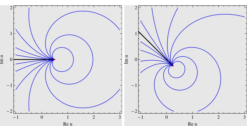
Figure 1.2: Complex rational solutions of the KdV equation: in the left panel
PT-symmetric solutions for c= 1, β = 2, γ = 3 andA = 1/2; in the right panel, we have taken c= 1, β = 2 +i2, γ = 3 and consequently A= (1−i)/4.
Two examples are shown in Figure 1.2, where we have traced in black the square-root branch cut of the velocity ˙u. On the second Riemann sheet, the orbits are the same but they are travelled in the opposite direction. Let us make a comment on the nature of the pointu =A. This point cannot be reached in any finite amount of time, and is an accumulation point for all the orbits. Moreover, obits can only approach this point along the direction of the line arg(u) = arg(γβ). This is a particular case of the general behaviour of orbits around algebraic zeros, see Section 1.3.4.
1.3.3.2 Trigonometric solutions
Now let us consider the factorization P(u) = (u−A)2(u−B) , which can be
obtained by taking
λ =− β
3γ, κ1 = A
2(βA−2c), κ2 =
A2
6 (3c−2βA) and B = 3c
The general solution in this case is
u(ζ) = A+ (B −A) cosh−2
1 2
√
A−B√λ(ζ−ζ0)
. (1.40) The phase portrait of these solutions can already show an interesting variety depending on the value of the parameters. It is interesting to classify the different possible behaviours of the orbits around the double zero u = A. This is clearly no longer a turning point. Instead, this point is characterised by the vanishing of both ˙u and ¨u(and therefore of all higher derivatives), meaning that the equation admits the constant solution u(ζ) =A. This is therefore a stationary point. For each of the two signs of the square root, the equation
˙
u=±λ(u−A)√u−B (1.41) now defines a smooth dynamical system in the neighborhood of u = A, which can be studied locally with the standard tools for two-dimensional real systems. It is convenient to separate u into its real and imaginary part, u=uR+iuI, uR,
uI ∈ R, so that (1.41) becomes:
˙
uR = +Reh√λpP(uR+iuI)i and u˙I = +Imh√λpP(uR+iuI)i,
(1.42) where we have restricted to the + sign in (1.41), since on the second sheet the orbits are the same, but simply travelled in the opposite direction. According to the classic classification reviewed in Appendix A, the behaviour of the solutions around u = A is determined by the eigenvalues of the Jacobian matrix, which here is simply
J(A) =
∂Re[√V(u)] ∂uR
∂Re[√V(u)] ∂uI
∂Im[√V(u)] ∂uR
∂Im[√V(u)] ∂uI u=A =
Re[dudpV(u)] −Im[dudpV(u)] Im[ d
du
p
V(u)] Re[d du
p
V(u)]
u=A . (1.43) with pV(u) = √λpP(u). We denote the eigenvalues of J(A) by j
1, j2. They
can be simply computed as
j1 =
d du
p
V(u)|u=A=
p
(a) (stable or unstable) star node, when ji ∈R .
(b) centre , when ji ∈iR .
(c) (stable or unstable) focus , in all other cases (ji ∈/ R, ∈/ iR).
Table 1.2: Small classification of the possible behaviour around the fixed point
u=A.
(with λ = −3γβ). We see that, while in a generic two-dimensional dynamical system there is no restriction on the eigenvalues, in the present case they are related by complex conjugation as a consequence of the Cauchy-Riemann equation satisfied by the real and imaginary parts of pV(u).
The possible behaviour at u =A is therefore restricted to the cases listed in Table 1.2. Let us consider them in order.
Case (a): solitary wave solutions When the choice of the parametersA,B
is such that ji ∈R, all the orbits (apart from a single orbit connecting the fixed
point to infinity, without passing through the turning point u = B 1) approach
asymptotically u=A for ζ → ±∞. They are natural complex extensions of the celebrated solitary wave solutions, or one-soliton solutions.
A PT+-symmetric example is shown in Figure 1.3, left panel. Notice that
rela-tions (1.39) imply that, if the parameters β, γ are chosen in a PT±-symmetric way according to Table 1.1, solitary wave solutions cannot break the symmetry: otherwise it would not be possible to have j1 ∈R. However, asymptotically
con-stant solutions exist also if the symmetry is missing from the start (when γ and
β are generically complex), as for example shown in Figure 1.4 below.
Case (b): complex periodic solutions Solutions obtained for ji ∈ iR
correspond to complex periodic orbits. These solutions have no real counterpart because in order to have periodic motion on the real axis one would need to have at least two turning points (this case will be presented below in 1.3.3.3). The phase portrait corresponding to complex periodic trigonometric solutions is presented in a PT+-symmetric example in Figure 1.3, right panel. Looking at (1.40), we see
that the period of these trigonometric solutions is given by T = √ 2πi
λ(A−B) =
2πi j1 .
1 This escaping orbit corresponds to the choice of Im(ζ
0 2 4 6 -2 -1 0 1 2 Re u Im u
0 2 4 6 8 10 12
-5 0 5 Re u Im u
Figure 1.3: Left panel: PT+-symmetric solitary wave solutions of the KdV equation with c= 1, β = 3/10, γ =−3, A= 4 andB = 2. Right panel: complex periodic PT+-symmetric solutions of the KdV equation with c = 1, β = 3/10,
γ = 3, A= 4, B = 2. The period is T = 2√15π.
We notice that this expression is the same for all orbits. In fact, this is a general feature of complex dynamical systems, which was noticed in Bender et al. [1999] in the case of the differential equations (1.12). The period of a closed orbit can be computed by a contour integral HCA duu˙ , where CA denotes the closed orbit under
consideration, encircling the point u = A. Provided ˙u is an analytic function, this quantity can be computed by integrating over any loop enclosing the point
u=A; therefore, the period is the same for all topologically equivalent orbits. In the present case the period can be re-obtained by using the theorem of residues:
T = I CA du ˙ u = I CA du p
λ(u−B)(u−A) =
2πi
p
λ(A−B). (1.45) With the same strategy, we can compute the energy (1.16) over one period:
ET =
I
Γ
H[u(ζ)]du
uζ
=
I
Γ
H[u]
√
λ√u−B(u−A)du =−π
r
βγ
3
A3
√
A−B. (1.46)
Case (c): open orbits Finally, whenji is neither real nor imaginary, all
so-lutions obtained with Im(ζ0)6= 2nπ,n∈Z1 are open orbits spiralling indefinitely
around the point A. Depending on the choice of Riemann section, these orbits fall into the fixed point or spiral out of it, corresponding to a stable or unstable focus, respectively. We depict an example in Figure 1.4. Notice that this type of behaviour is associated to orbits breaking PT-symmetry. Such orbits correspond to taking generic complex values for A, and are accompanied by PT-symmetric conjugate orbits corresponding to the choice A∗.
0 5 10 15
-10
-5 0 5 10
Re u
Im
[image:40.595.181.437.293.545.2]u
Figure 1.4: Complex trigonometric solutions of the KdV equation with “spon-taneously broken” PT-symmetry. c = 1, β = 3/10, γ = 3, A = 4 +i/2 and
B = 2−i, meaning that this family of orbits break the PT+-symmetry of the
equation. All orbits of this type are in the present case open.
Relation with PT-symmetry breaking In summary, we have found that
PT-symmetric orbits are always either periodic or correspond to solitary waves. Orbits that break the symmetry spontaneously are very different, in particular
they are always open. This is very reminiscent, in spirit, of the findings of Bender
et al. [1999] that we have summarised in Section 1.2.2.
-10 -5 0 5 10 15 20
-10
-5 0 5 10
Re u
Im
[image:41.595.181.439.187.440.2]u
Figure 1.5: Detail of a trigonometric solution of the complexified KdV equation with broken PT-symmetry. Here we have taken c = 1, β = 3/10, γ = 3 + i/2,
A= 4,B = 2. The pointu= 4 behaves like afocus. This solution is characterised by Im(ζ0) = 6.
When, on the other hand, the symmetry isexplicitly broken, namely we take generic complex values for β,γ, solutions are almost always open, with the fixed point behaving like a focus (see Figure 1.5 for a detail). However, there are still examples of periodic or asymptotically constant orbits. They are associated to a subset of all possible choices for A, obtained by imposing the condition
Re(
r
λ(3A∗+3c
β )) = 0 or Im(
r
λ(3A∗+ 3c
β)) = 0. (1.47)
-4 -2 0 2 4 -2 -1 0 1 Re u Im u
-40 -20 0 20 40
-40 -20 0 20 Re u Im u
Figure 1.6: Two solutions of the non PT-symmetric complex KdV equation, where the parameters have been finely tuned in order to obtain a solitary wave solution (left panel), or a periodic solution (right panel). The choice of parameters is: Left: c = 1, β = (16−4i)/17, γ = −3, A = 4 +i, B = −5−5/4i ; Right:
c= 1, β = (−8 + 2i)/17, γ =−3 and A= 4 +i, B =−14−7/2i .
1.3.3.3 Elliptic solutions
Finally, let us consider the general case of a potentialP(u) = (u−A)(u−B)(u−C) with three distinct turning points (the relation between A, B, C and the other parameters is given in (1.32) ). In this case the solution reads:
u(ζ) =A+ (B−A) sn21
2
√
B−A√λ(ζ−ζ0)
A−C
A−B
, (1.48)
where sn(z|m) is Jacobi elliptic function.
In the PT-symmetric situation, this corresponds to the celebrated cnoidal solution of KdV equation, playing an important role in the initial value problem over a periodic domain. This solution is real and periodic, oscillating between two turning points. In Figure 1.7, we present the natural extension of the cnoidal solution to the complex plane, where it is accompanied by a family of complex periodic orbits. Apart form a single real orbit running on the positive real axis between u=C and u= +∞, all orbits again share the same period, given by
ω1 =
8
√
B−A√λK
A−C A−B
-5 0 5 10
-4
-2
0 2 4
Re u
Im
u
Figure 1.7: PT-symmetric complex elliptic solutions of the KdV equation with
A= 1, B = 3, C = 6, c= 1, β = 3/10, γ =−3 for different values of Imζ0.
Being an elliptic function, the solution is in fact doubly periodic. The second period, which in the example shown in Figure 1.7 would be purely imaginary, is given by
ω2 =i
16
√
B−A√λK
C−B A−B
. (1.50) When the symmetry is broken, we observe quite interesting trajectories which densely fill each of the two sheets covering the complex u-plane. An example is plotted in Figure 1.8. The trajectory appears to repeat indefinitely the same manoeuvre around the turning points.
A simple explanation of the space-filling character of these orbits is that, when the symmetry is broken, the two periodsω1,ω2become genuinely complex. When
the imaginary parts of the two periods are not commensurable, the problem is equivalent to motion on a torus with two incommensurable frequencies: it is a classic result that this quasi-periodic motion is dense on the torus (see for example Arnol’d [1989]). As noticed in Anderson et al. [2011]1, there are still sparse
examples of periodic orbits with a broken symmetry. These more complicated
1Bender et al were considering simple potential systems. For an illustration of some of these
orbits, see Anderson et al. [2011], where also quartic potentials and more general non-elliptic
-4 -2 0 2 4 6 8
-6
-4
-2
0 2 4 6
Re u
Im
u
0 2 4 6 8
-4
-2
0 2 4
Re u
Im
[image:44.595.109.509.140.343.2]u
Figure 1.8: Spontaneously broken PT-symmetric complex elliptic solution of the
KdV equation for Imζ0 = 6 withA= 4,B = 5−i/2,C = 1+i/2,c= 1,β = 3/10
and γ = 3. The left panel shows the trajectory for −64≤ ζ≤ 18 solid (red) and 18< ζ ≤ 200 dashed (black). In the right panel: −200 < ζ <1400. Notice that this is a single, space-filling trajectory.
periodic solutions are obtained when the two elementary periods, despite being both complex, happen to have imaginary parts commensurate to each other, in the sense that there exist two integersm,n ∈Zsuch that nω1+mω2 ∈R. This
can also be rewritten as (see Anderson et al. [2011]) Im(mω1+nω2) = 0→
m n =−
Imω1
Imω2
. (1.51) It is important to remark that, similar to what was seen in the case of trigono-metric solutions, these special obits exist only for a lower-dimensional subset of the parameter set, and, for a generic choice of parameters, we again see a strong connection between the periodicity of the orbits and PT-symmetry.
-10 0 10 20 30 40 50
-20
-10
0 10 20 30 40
Re u
Im
u
-10 -5 0 5 10
-10
-5
0 5 10
Re u
Im
u
Figure 1.9: BrokenPT-symmetric complex elliptic solutions of the KdV equation
for Imζ0 = 6: in the left panel, A = 1, B = 3, C = 6, c = 1, β = 3/10 and
γ = 3 + 2i for −200 ≤ ζ ≤ 200; in the right panel, A = 1, B = 2 + 3i, C = 6,
c= 1, β = 3/10−i/10 and γ = 3 for −200≤ζ ≤200.
1.3.4
Deformations of the KdV equation I: the
PT
+-symmetric
deformation
Let us come to the first type of deformation. Before presenting some examples, let us make a general comment. From (1.34), we have
ζ −ζ0 = exp
iπ
2(ε+ 1)(ε−1)
Z
du 1
[λεP(u)]
1 1+ε
. (1.52) In general, the best we can do is computing the integral in terms of a complicated function F(u), such that
ζ−ζ0=F(u). (1.53)
While this relation is in general not invertible, we can easily obtain the orbits numerically by plotting them as lines of constant Im(ζ0). The following plots
Behaviour at general algebraic points As we have anticipated, this defor-mation leaves unchanged the position of the three zeros of the potential A, B,
C, but changes their characteristics depending on the value of ǫ. The qualitative behaviour of the solutions of (1.34) around one of these roots (which we denote generically as k) can be understood by considering the simple model equation
˙
u=b(u−k)α, (1.54) where
α = σ
ǫ+ 1, (1.55) and σ ∈ {1,2,3}is the order of the zero of P(u) atu=k. The solution of (1.54) in general lives on an infinitely-sheeted Riemann surface, with a branch point at u = k. Obviously we expect the behaviour to change abruptly depending on whether α >1 or α < 1. Notice that the “regular case” α= 1 stands alone: the possible behaviours for α = 1 are the ones classified in Table 1.2. Solving (1.54) for α6= 1 we find
u(ζ) =k+
−αb(ζ−ζ0)
1
1−α
, (1.56) where the value of Im(ζ0) labels different orbits. We notice that some solutions
(identified by Im(ζ0) = 0) are simply outgoing or ingoing rays, with the number
of rays on every Riemann sheet depending on α. They are described by arg(u−k) = −arg(b
α) +
2nπ
1−α, n ∈Z (outgoing) , (1.57)
arg(u−k) = −arg(b
α) +
(2n+ 1)π
1−α , n ∈Z, (ingoing) . (1.58)
The difference between the cases α > 1 and α < 1 can be described as follows. For α > 1 and for every value of Im(ζ0), every orbit approaches the point u=k
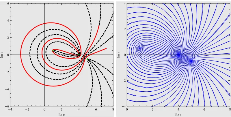
Figure 1.10: Complex PT-symmetric rational solutions of the deformed KdV
equation withc= 1,β = 2 andγ = 3 for the deformed modelH+
−1/2,
correspond-ing to the behaviour (1.54) with k= 1/2 and α= 6.
pointu=k, and neighbouring orbits form a saddle-point like pattern (see Figure 1.11).
The deflection of the orbits in the presence of such “generalised turning points” was recently discussed in the paper Bender & Hook [2014]. In this paper the rays (1.57-1.58) are referred to as “separatrix trajectories” and we adopt this terminology in the following. They are a new feature which does not exist in the undeformed case, and we will see that they divide the phase portrait in different sectors.