The Value of Control and the Costs of Illiquidity

City, University of London Institutional Repository

Citation:

Illiquidity. Journal of Finance, 70(4), pp. 1405-1455. doi: 10.1111/jofi.12207

This is the accepted version of the paper.

This version of the publication may differ from the final published

version.

Permanent repository link:

Link to published version:

Copyright and reuse: City Research Online aims to make research

outputs of City, University of London available to a wider audience.

Copyright and Moral Rights remain with the author(s) and/or copyright

holders. URLs from City Research Online may be freely distributed and

linked to.

City Research Online: http://openaccess.city.ac.uk/ [email protected]

The Value of Control and the Costs of Illiquidity

Rui Albuquerque and Enrique Schroth

Forthcoming,Journal of Finance

ABSTRACT

We develop a search model of block trades that values the illiquidity of control-ling stakes. The model considers several dimensions of illiquidity. First, following a liquidity shock, the controlling blockholder is forced to sell, possibly to a less e¢ cient acquirer. Second, this sale may occur at a …re sale price. Third, absent a liquidity shock, a trade occurs only if a potential buyer arrives. Using a structural estima-tion approach and U.S. data on trades of controlling blocks of public corporaestima-tions, we estimate the value of control, the blockholders’ marketability discount and the dispersed shareholders’illiquidity-spillover discount.

High ownership concentration is a predominant phenomenon in the corporate world. In many

countries, including the United States, evidence suggests that high ownership concentration is

pervasive in public corporations.1 _{By de…nition, ownership concentration is also an integral}

part of privately held corporations.2 _{In this paper, we study the value of controlling blocks}

of shares in public corporations, contributing to the understanding of the costs and bene…ts

of concentrated ownership. An inherent di¢ culty in valuing controlling blocks of shares is the

illiquidity of the market. Theoretically, illiquidity in the market for controlling blocks is a cost

that a¤ects the block value, possibly in a nonlinear way. Empirically, illiquidity reduces the

number of observations available to the econometrician and constrains the empirical strategy

of estimating the block value. We provide a model of the trading and pricing of controlling

blocks in an illiquid market with search frictions. We argue that block-trading events convey

information that identi…es the model parameters and allows the estimation of the value of

control.

The model’s main premise is that a controlling blockholder of a public corporation a¤ects

the value of the …rm’s assets (Holderness and Sheehan (1988); Barclay and Holderness (1989);

and more recently Pérez-González (2004)). Therefore, given the choice, the controlling

block-holder will only sell to a bidder who can increase asset value. In addition, we assume that the

controlling blockholder is forced to sell if hit by a liquidity shock, in which case he may sell to

a party that creates less asset value and be paid a …re sale price. The potential absence of a

bidder at any given time further increases the illiquidity of the block. These frictions give rise

to amarketability discount on the value of the block. Additionally, the possibility that the new

blockholder may decrease asset value introduces a discount on the dispersed shares traded in

the stock market. We name this novel e¤ect the illiquidity-spillover discount.

The estimation of the marketability and the illiquidity-spillover discounts is notoriously

dif-…cult because they require a counter-factual analysis: what should the price be absent search

frictions? The structural estimation adopted in the paper uses the model’s pricing equations

suc-cessfully identify the parameters of these pricing equations. In particular, since the pricing will

di¤er depending on whether or not the trade was caused by liquidity shocks, the model must

identify ex post the reasons for trading. These reasons are unobservable to the econometrician.

One contribution of this paper is to show that it is possible to identify the model’s

parame-ters by using the valuations of two di¤erent types of shareholders during a block trade: the

blockholders’ valuation implicit in the negotiated block price and the dispersed shareholders’

valuation revealed in the exchange share price.

In the model, a liquidity shock is the realization of a random variable with a Bernoulli

distribution that forces blockholder turnover. Following a liquidity shock, the block is sold at a

…re sale price equal to a fraction of the buyer’s valuation. In contrast, the dispersed shareholders

only care about the discounted value of future cash ‡ows under the new blockholder and not

the …re sale price. This price di¤erence allows us to identify …re sale discounts.

In the absence of a liquidity shock, the block changes hands only if a potential new

block-holder arrives and can generate more cash ‡ow. In this case, block and share prices di¤er partly

because liquidity shocks penalize blockholders more than dispersed shareholders, who are

un-a¤ected by the lower expected …re sale price in a future sale. In short, our model is able to

fully exploit the data by identifying liquidity shock probabilities not only out of the frequency

of trades with negative price reactions, but also the block vs. share price di¤erences that exist

whether or not liquidity shocks have occurred.

We estimate an average probability of getting a liquidity shock within one year of 20%, and,

conditional on a liquidity shock, an average …re sale discount of 8% of the block value.3 _The

estimated probability of meeting a potential buyer within one year is 43%. We …nd that the

marketability discount, which is a non-linear function of these three estimates, is on average

13% of the block value, with a standard deviation of 22%. The spillover e¤ect of the block’s

illiquidity on the dispersed shares is on average 2.1% of the share price.4

A selection bias in our estimates may arise if not all liquidity shocks lead to a …re sale. That

a …re sale, for example, using the block as collateral for a loan. We argue that this selection

bias leads to downward-biased estimates of the probability of a liquidity shock. In addition, our

reduced form approach to …re sale prices may lead to upward-biased estimates of the …re sale

price. That is, what we call a …re sale price is likely to be the maximum payout among many

alternative ways of reacting to the liquidity shock, which include, for example, the arrival of a

private equity …rm supplying liquidity. Because the marketability and the illiquidity-spillover

discounts are decreasing in the …re sale price and increasing in the probability of a liquidity

shock, these biases lead to the underestimation of the discounts. Our approach, therefore, gives

a conservative estimate of the discounts we study.

We allow the probability of a liquidity shock and the …re sale price to vary across deals

as a function of economy-wide and deal-speci…c determinants of liquidity in order to match

the observed variation in the block and exchange share prices. Economy-wide determinants

of liquidity appear to capture unobserved variation in the probability of a liquidity shock,

whereas …rm and industry characteristics appear to capture unobserved variation in …re sale

values. We …nd that the probability of a liquidity shock is increasing in the Fontaine and Garcia

(2012) measure of aggregate funding illiquidity, and decreasing in GDP growth and the stock

market return. However, the probability of a liquidity shock is high when GDP growth and

market returns are high and the yield curve is steep. Our interpretation is that macroeconomic

expansions increase block holder liquidity via their balance sheet e¤ects but may also trigger a

preference for cash if they bring good investment opportunities when outside funding is costly.

The block’s …re sale value decreases with the degree of asset speci…city of the target …rm’s

industry and with the target …rm’s leverage relative to that of its industry. The evidence

that the state of the aggregate economy determines …rm-speci…c liquidity complements the

work of Chordia, Roll, and Subrahmanyam (2000) and Bao, Pan, and Wang (2011), who …nd

commonalities in asset-speci…c liquidity measures.

We discuss the robustness of our results to other possible motives for trading. Trading could

to increase share value, the resulting drop in the dispersed shareholders’ valuation could be

misinterpreted as a the consequence of a liquidity trade. We show that the use of data on the

blockholders’valuation, together with data on the dispersed shareholders’valuation, allows us

to distinguish these two types of trades. Intuitively, liquidity trades are bad events for the block

sellers whereas private bene…ts trades are good events. Therefore, the two trading reasons have

opposite e¤ects on the blockholder’s valuation.

The literature has considered alternative ways of measuring the value of control. One

ap-proach is to look at the voting premium, measured directly as the price di¤erence of shares with

di¤erent voting rights (e.g., Masulis, Wang, and Xie (2009)), or indirectly as deviations from

put-call parity (Kalay, Karakas, and Pant (2012)) and equity-loan values (Christo¤ersen et al.

(2007)). By studying per share prices, these approaches measure the marginal value of control.

Because in our data we have the total price of a block, we are able to comment on the total

value of control. Moreover, our structural approach allows us to isolate the cost of illiquidity

from the total e¤ect of control, which also includes the increase in security bene…ts.

The paper that is closest to ours is Albuquerque and Schroth (2010). They estimate private

bene…ts of control that result from diverting cash ‡ow, whereas we are the …rst to estimate the

costs of illiquidity embedded in the value of control. Albuquerque and Schroth (2010) focus on

smaller controlling blocks as they expect that private bene…ts of control are more likely to have

a …rst order e¤ect on valuations and trading decisions in these blocks. Illiquidity has no role in

their model. In contrast, our main premise is the opposite: for larger blocks, illiquidity is more

likely to have a …rst order e¤ect whereas incentive alignment between controlling and dispersed

shareholders should imply zero private bene…ts of control derived from the …rm’s cash ‡ows.

The literature started by Barclay and Holderness (1989) also looks at the total value of control.

These papers do not consider the costs of illiquidity associated with large blocks.

There is a vast literature on the pricing of illiquid assets (see Amihud, Mendelson, and

Pedersen (2005) for a comprehensive survey). Longsta¤ (1995) measures the marketability

as opposed to trading restrictions and allows the owner of the shares to have an in‡uence over

the cash ‡ows of the …rm. Du¢ e, Garleanu, and Pedersen (2005, 2007) present search models

of over-the-counter markets with atomistic investors. In these papers there is no controlling

shareholder that can a¤ect the value of assets and discounts result from a pure search cost. In

our paper, liquidity costs also arise from the possibility of having to sell the block at …re sale

prices and to a less e¢ cient buyer.

Related theoretical work shows that concentrated ownership induces illiquidity in the …rm’s

exchange traded shares (see Demsetz (1968), Holmstrom and Tirole (1993), and Bolton and von

Thadden (1998)).5 This literature focuses on the price implications of a reduced ‡oat. Instead,

by studying block-trading events where the ‡oat is unchanged, we are able to focus on the pricing

implications of liquidity shocks to large blockholders. Kahn and Winton (1998) and Maug

(1998) argue that, if blockholders obtain value-relevant information from their monitoring, then

the resulting adverse selection problem when blockholders trade their shares lowers liquidity

(see also Edmans and Manso (2011)). We believe that the size of the controlling blocks studied

in this paper and the fact that blocks are not partitioned suggest that this cause for illiquidity

is of second order in our exercise and should not a¤ect our results.

Vayanos and Wang (2007) and Weill (2008) study illiquidity spillovers in search models with

multiple securities. They …nd that search frictions can lead to higher prices in more liquid

assets (i.e., with lower search times) despite the fact that the assets have identical cash ‡ows.

Chordia, Sarkar, and Subrahmanyam (2011) …nd evidence of liquidity spillovers across size

portfolios by inspecting lead-lag cross-correlation patterns. Aragon and Strahan (2009) use the

Lehman Brothers bankruptcy to show that stocks traded by hedge funds connected to Lehman

experienced greater declines in market liquidity. The illiquidity spillover studied in this paper

instead looks at how the liquidity shocks to the controlling blockholder spill over to the value

of the shares held by dispersed investors of the same …rm.

The paper proceeds as follows. SectionI presents preliminary evidence on controlling block

II presents the search model that we use to price controlling blocks and dispersed shares.

Section III describes the empirical strategy. SectionIV summarizes the data used and Section

V presents the main results. SectionVI discusses additional tests and SectionVII concludes.

I. Preliminary Evidence on Controlling Block Trades

In a block trade, the incumbent holder of a block of shares on a target …rm sells the entire

block to a rival blockholder. Simultaneously, dispersed shareholders of the same target …rm

react to the news of the trade leading to a change in the price of the exchange-traded shares.

This information is summarized respectively in the block premium (BP) paid by the acquirer

of the block and in the cumulative abnormal (announcement) return (CAR) on the

exchange-traded shares.

Our data comprise 114 U.S. disclosed-value acquisitions of blocks of more than 35% but less

than 90% of the shares of a company between January 1, 1990, and December 31, 2010. These

data are described in detail in SectionIV. We measureBP as the ratio of the unit block price

to the exchange-traded share price 21 trading days before the block trade announcement. We

measure CAR as the ratio of the exchange-traded share price 2 trading days after the block

trade announcement to the exchange-traded share price 21 trading days before the

announce-ment. This choice of event window follows Barclay and Holderness (1989) and others, and is

meant to capture the full e¤ect of market expectations about the unfolding block trade and the

corresponding e¤ect of the change of control on security bene…ts.

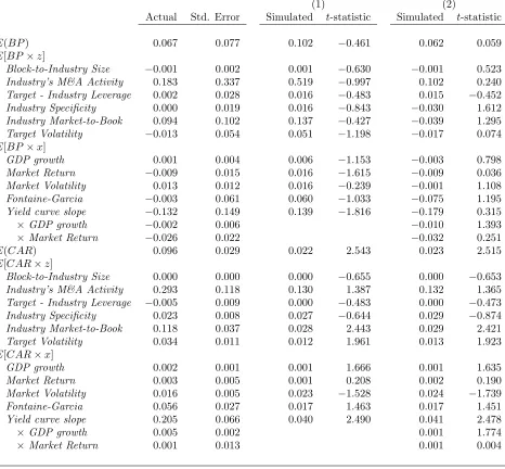
Figure1shows the scatter plot ofBP andCARin our sample. There are several noteworthy

features. First, the average BP in our sample is 6:8% and the average CAR is 9:6%. Despite

these positive means, 47% of deals have negative BP and 42% of deals have negative CAR.

Second, BP and CAR are positively correlated, with a correlation coe¢ cient of 0:37. This

strong association captures the fact that most trades are concentrated in two regions of the

scatter plot, with 74% of the trades with positiveCAR exhibiting a block premium and75% of

that, for most majority-block trades, dispersed shareholders and blockholders either gain or

lose simultaneously.

<INSERT FIGURE 1ABOUT HERE>

How are these data informative of liquidity shock probabilities? Consider the subsample of

trades where dispersed shareholders respond negatively to the announcement (i.e., CAR <0).

For these deals, a decline in the shared security bene…ts may have been caused by either a

liquidity shock that forced the incumbent blockholder to sell, implying also losses to the

block-holder (i.e., BP <0) or a gain in private bene…ts at the expense of the dispersed shareholders,

so that BP >0.

Based on this distinction, one approach to identify the probability of liquidity shocks would

be to treat all deals with CAR < 0 and BP < 0 as having been caused by such shocks and

then specify a reduced-form probabilistic regression model to explain the event that CAR <0

and BP < 0. However, this approach introduces biases by neglecting the fact that deals with

CAR >0can also be informative of liquidity shocks. First, the incumbent blockholder may have

been hit by a liquidity shock but found a white knight that provided liquidity while increasing

shared security bene…ts. Second, forward-looking block and share prices must incorporate the

possibility of liquidity shocks in the future, even for deals that were not caused by liquidity

shocks. Indeed, 30% of our sample contains deals where blockholders gain more than

share-holders (BP > CAR >0). While these deals were most likely caused by an increase in security

bene…ts, the transaction prices embedded inBP andCAR are likely to also re‡ect information

about liquidity shocks.

We extract two conclusions from this discussion. First, because block trades by and large

imply either simultaneous gains or losses to blockholders and dispersed shareholders, the main

reasons for trading in our data must be increase in security bene…ts or sales forced by liquidity

shocks. Second, a successful approach to identify the probability of liquidity shocks must

or negativeCAR. Moreover, due to their forward-looking nature, the prices in di¤erent scenarios

will incorporate information about the same parameters. Essentially, any deal in the data can

potentially be informative of liquidity shocks if structurally modeled.

The di¢ culties in identifying illiquidity-driven trades carry over to estimating the value of

control. Because the block premium in deals with positive CAR incorporates both shared

se-curity bene…ts and illiquidity costs, estimation of illiquidity costs requires a way to disentangle

these two opposing e¤ects. The model developed in this paper proposes an economic

mech-anism whereby illiquidity costs have di¤erent e¤ects on blockholder valuations and dispersed

shareholder valuations. The structural estimation infers these illiquidity costs by matching the

data on BP and CARto the model’s predictions of these prices.

II. A search theory of block trades

This section presents an estimable model of the valuation of a controlling block that includes

a proportion <1of the shares of a …rm, and the valuation of the 1 remaining shares held

by dispersed shareholders. Time is discrete and investors have discount factor <1.

A. Blockholder’s value

The current block owner is called the incumbent and is denoted byI. The …rm’s cash ‡ow

is a discrete random variable that takes values on a grid_f 1; :::; Ng:Without loss of generality,

we assume that m > l for any m > l. Let Il denote the …rm’s cash ‡ow in state l when

I is in control. It evolves stochastically according to the conditional probability distribution

Pr [ 0 = mj = l] =qlm with qlm >0 and PNm=1qlm = 1 for every l = 1:::; N, where the prime

denotes next period values. We assume that the transition matrix induced by the conditional

probabilities qlm is monotone.

Denote byv I

l the incumbent’s per share value of the block at Il. This value includes the

shared security bene…ts and illiquidity costs to the blockholder. The blockholder also obtains

but rather from social prestige and network building in the case of an individual blockholder

or from valuable synergies in the case of a corporate blockholder. We assume per share private

bene…ts are constant across incumbent and rival and equal to B.

At the beginning of every period, I may face a liquidity shock with probability . If a

liquidity shock occurs, then I is forced to sell at a …re sale price to a rival blockholder denoted

by R. The …rm’s cash ‡ow under the rival is denoted by R

m and is drawn from the same

transition matrix induced by qlm given the current state l. We do not model how the block

trades following a liquidity shock. Instead, we specify the …re sale price in reduced form as

v R_m . The parameter summarizes the owner’s liquidity and the parameter summarizes

the asset’s liquidity. Therefore, the ex ante block price upon a liquidity shock is

Lv_l = N

X

k=1

qlkv( k): (1)

If a liquidity shock does not occur, the incumbent is matched with a potential buyer with

probability . The parameter is a measure of market thinness. We assume trading is the result

of Nash bargaining, where the seller’s relative bargaining power is 2 [0;1]. If bargaining is

successful, R pays the prices I_k; R_m and getsv R_m plus the private bene…ts.

The value of the block to the incumbent, v, is the sum of the current cash ‡ow, I l, the

continuation value in the absence of a liquidity shock, ~v, and the liquidation value, Lv_l, that is,

v I_l = I_l +

"

(1 ) N

X

k=1

qlkv~l Ik + Lvl

#

: (2)

The continuation value absent a liquidity shock plus private bene…ts equal

~

vl Ik +B = N

X

m=1

qlmmax s Ik; Rm ; v kI +B + (1 ) v Ik +B : (3)

The incumbent has an option to sell the block for s I_k; R_m to a higher valued blockholder.

Under Nash bargaining,s I_k; R_m solves

max

s s v I

k +B v Rm +B s 1

:

When a there are gains from trade v I

k < v Rm , the solution is

Otherwise, no trade occurs and I remains the blockholder with valuationv I_k +B. From (4),

the block price must compensate I for the value attained by not selling plus I’s fraction of the

added surplus that results from R taking over.

The next proposition characterizes the functionv( ). The proof is provided in the appendix.

Proposition 1 The value function v exists, is unique, and is strictly increasing in .

The property that v is strictly increasing implies that it is optimal to sell the block if and

only if I

k< Rm. Therefore, we can simplify ~v as

~

vl I_k =v I_k + X m>k

qlm v R_m v I_k : (5)

The last term on the right hand side of equation (5) is the value of the option to sell. The

fraction of the option to sell accrues toI but can only be captured if a rival appears, which

occurs with probability . Note that it is worth selling to an incrementally better rival because

all future increases in value that result from a sale by the rival are already properly valued in

v and there are no …xed costs of selling.

The model’s property that the block is sold if and only if I

k < Rm (rather than if and only if

v I_k < v R_m ) is extremely useful. As we show in Appendix B, this property implies that we

can solve the …xed point problem de…ning v (equations (2) and (5)) via a perfectly identi…ed

system of linear equations that only requires inverting a matrix. Proposition 1 guarantees

that this matrix inverse exists. This property follows from the assumption that R and I are

heterogeneous only with respect to the cash ‡ow they generate. Any two blockholders generating

the same cash ‡ow have equal security bene…ts, v( ): Without this property, we would have

to solve the value function …xed point problem simultaneously with the decision rule that

v I_k < v R_m (see Afonso and Lagos (2012) for a similar result).

B. Dispersed shareholders’value

The model assumes complete information by all investors. Therefore, dispersed shareholders

stock market at the share price p such that

p I_l = I_l +

"

(1 ) N

X

k=1

qlkp~l Ik + L p l

#

: (6)

Dispersed shareholders know that with probability 1 there is no liquidity shock and the

block is sold if and only if a rival is present and generates higher cash ‡ows. The share price

absent a liquidity shock, p;~ is given by

~

pl Ik =p Ik + N

X

m=1

qlmmax p Rm p Ik ;0 : (7)

Dispersed shareholders also bene…t from I’s option to sell. Further, we will show that p( ) is

increasing in , which implies that I’s decision rule to sell is e¢ cient. This result is appealing

because it is consistent with the correlation between the block premium and announcement

return documented in Section I. The last component of the share price is the expected share

price if a liquidity shock occurs,

Lp_l = N

X

k=1

qlkp( k): (8)

Dispersed shareholders di¤er from blockholders in three ways. First, they do not receive

any private bene…ts from holding the stock. Second, dispersed shareholders are able to extract

all the value from the option to sell because they act in a competitive market. Indeed, they do

not bargain over the gains from trade. Third, dispersed shareholders are not hit with liquidity

shocks and are not forced to sell at a …re sale price. However, they lose if, upon a liquidity

shock, the incumbent sells to a rival that generates lower cash ‡ows. These di¤erences are

critical for the model to identify the illiquidity cost parameters.

The next proposition characterizes the function p( ).

Proposition 2 The value function p exists, is unique, and is strictly increasing in . Also,

p( )> v( ) for any whenever >0 and <1, or >0 and <1.

As in Bolton and von Thadden (1998), dispersed shareholders value security bene…ts more

blockholders that have less impact on dispersed shareholders. Speci…cally, when the probability

of a liquidity shock is strictly positive, …re sale discounts a¤ect blockholders more than they do

dispersed shareholders if <1. Likewise, when >0, selling to a more e¢ cient rival bene…ts

the dispersed shareholders more because <1. The model therefore relies on private bene…ts to

explain why blockholders may value shares of the target …rm more than dispersed shareholders.

C. The block premium and the price reaction to the trade

Conditional on a trade, the block price is v R_m if a liquidity shock occurs, and s I_k; R_m

otherwise. The block premium is de…ned as the ratio of the share block price to the

per-share pre-trade price:

BP I_k; R_m

8 > < > :

v( R m)

p( I k)

1; if a liquidity shock occurs,

s( I k; Rm)

p( I k)

1; else.

(9)

The price reaction to the block trade announcement is de…ned by:

CAR I_k; R_m p R m p I

k

1: (10)

Note that CAR < 0 signals liquidity shocks: it only occurs if the block is traded after a

liquidity shock and the new block owner generates lower cash ‡ow. However, the converse is

not true: CAR >0 occurs following a liquidity shock if the randomly matched rival produces a

higher cash ‡ow. The next section discusses how the probability of a liquidity shock is identi…ed

despite this di¢ culty.

III. Empirical strategy

The unit of observation in our data is a block trade indexed byi. The dependent variables

areCARi and BPi. Our model allows us to construct theoretical counterparts to these for each

deal as a function of the parameters of interest: the owner’s liquidity shock probability, , the

asset’s liquidity parameter, , market thinness, , the blockholder’s private bene…ts,B, and the

model identi…es these parameters from the data. These parameters are constant in the model

for each trade and we will treat them as such in the empirical estimation. However, there is no

model-imposed restriction on how these parameters vary across trades. We then discuss how

we specify variation across trades for some of these parameters. Finally, the section describes

the estimation method.

A. Identi…cation

We develop a novel identi…cation strategy to estimate a search model that uses the di¤erences

in the valuation of blockholders, BP, and of dispersed shareholders, CAR, at the time of the

block trade. Traditional identi…cation strategies in search models require either information on

the time between two trades of the same block or contemporaneous trades of di¤erent blocks

on the same stock (Feldhütter (2012)). Neither alternative is feasible to us.

A.1. Identi…cation of

The model de…nes three main regions in the (CAR; BP) space that can be used to

iden-tify liquidity shocks. First, the model infers that trades exhibiting a negative price reaction

(CAR <0)must have been caused by a liquidity shock.

Second, the model infers that a liquidity shock cannot have occurred if the trade resulted

in a block premium that surpassed the increase in dispersed shareholders’s valuation, BP

CAR >0:To see this note that v R v R < p R , for any R_{, so that any trade caused}

by a liquidity shock must have

BP = v R

p( I₎ 1< p R

p( I₎ 1 =CAR:

Hence, deals in Figure 1 with BP CAR > 0 are voluntary trades where shared bene…ts

increased.

Third, for the remaining deals in the sample with CAR > 0 and CAR > BP, the model

assigns an ex-post probability that a liquidity shock occurred that is equal to

Pr [ 0 _{> lj = l]}

The numerator describes the probability that a trade results from a liquidity shock to the

incumbent that nonetheless yields an increase in shared bene…ts. The denominator describes

the probability that a trade occurs and there is an increase in shared bene…ts.

Interestingly, the model allows us to extract information about even for those deals that

it predicts were not caused by a liquidity shock, that is, in the region where BP CAR > 0.

To see this, consider panel (a) of Figure 2, which plots the simulated mean valuation spread

BP CAR conditional on BP CAR > 0; against . The parameter values are close to the

actual estimates given below, but the plot has an identical shape for a wide range of values.

The valuation spread is decreasing in . Intuitively, this spread re‡ects the fact that these

shocks penalize blockholders more than dispersed shareholders because blockholders have a

lower expected …re sale price. Interestingly, the valuation spread is informative (i.e., steeper)

when liquidity shocks did not occur ex post (i.e., BP > CAR >0) and were unlikely ex ante

(i.e., low ).

<INSERT FIGURE 2 HERE>

A.2. Identi…cation of and

Estimation of relies on the fact that …re sale prices a¤ect only the blockholders’value,v,

but not the share price, p. Therefore, when a liquidity shock has occurred, the model primarily

assigns the variation in block prices that is not associated with variation in the price reaction

to variation in . In addition, it is possible to infer variation in even in deals that the model

predicts that there was no liquidity shock. Panel (b) of Figure 2 indicates that the valuation

spread increases with conditional on BP CAR > 0. The intuition is that, in this region,

the block premium incorporates the likelihood of a future …re sale and therefore is increasing

in , whereas the announcement return is una¤ected by .

Market thinness, , a¤ects directly the value of the option to sell to a high-valued rival. Like

; BP and CAR increase with . However, as depicted in panel (c) of Figure 2, BP CAR

relies on the fact that, unlike , it cannot explain the occurrence of negative price reactions.

A.3. Identi…cation of B and

The size of private bene…tsB has an important role in capturing variation in the data where

CAR > 0. The choice of B faces the following trade-o¤: too low and the estimation may fail

to match the average block premium in deals where BP CAR > 0; too high and it may

misclassify trades with low BP and CAR > 0 as due to liquidity shocks. For this reason, we

add some ‡exibility to the functional form of B, allowing private bene…ts to vary across deals

but, to remain consistent with the model, not across blockholders in the same deal.

To identify the bargaining parameter, , the model relies on the fact that a¤ects the block

price but notCAR. While these facts are also true for the asset liquidity parameter, , there is

one important di¤erence between and : has a …rst order e¤ect on the block price absent

a liquidity shock through the value of the option to sell, whereas has a …rst order e¤ect on

the block price in the presence of a liquidity shock.

B. Modeling liquidity

In our estimation, as well as in the model, and are constant for each deal but allowed to

vary across deals. We model the cross-sectional variation in and using parametric logistic

functions:

(xi; ) = exp (x 0 i ) 1 + exp (x0

i )

; (12)

(zi; ) = exp (z 0 i )

1 + exp (z0_i ): (13)

By construction, the logistic function guarantees that and are bounded between 0 and 1. In

these functions,xi and zi are vectors of exogenous determinants of liquidity shocks and …re sale

prices, respectively, whereas and are vectors of …xed sensitivities to be estimated. As we

describe in detail in Section IV, xi includes variables that describe the state of liquidity, such

in zi capture variation in the traded blocks’ …re sale value, including proxies for industry

redeployability and asset speci…city. Variation in xi and zi across deals allows us to estimate

and through the variation they produce on BP and CAR.

While varies with xi and varies with zi, the model and the estimation constrain and

to be constant over time for each deal i. This assumption is equivalent to assuming that

blockholders and dispersed shareholders display a myopic attitude towards changes in these

quantities. The ability of the model to reasonably …t the data suggests that our assumption

may not be too restrictive and the reason may be that the variables we include in xi and zi are

quite persistent. Ideally, the model and estimation would allow forxiandzito be state variables

in the investors’problems and for investors to change their valuations as their forecasts of and

changed. We do not pursue this approach because it is highly computationally demanding,

but allowing for time variation in and is a goal for future research.

C. Estimation

C.1. Algorithm

For each deal, we estimate the conditional probabilities qlm using annual cash ‡ow data at

the target …rm’s 3-digit SIC level. We obtain an industry cash ‡ow grid and its associated

Markov transition matrix from the discretization of the estimated AR(1) process of the

log-detrended cash ‡ow time series. We construct a …rm-level grid from the industry grid assuming

constant price to cash ‡ow ratios. The use of industry data for the regressions guarantees, with

its longer time series, more precise estimates. More details can be found in Appendix C.

We set the discount factor to 1=1:1. This choice of a 10% discount rate includes a

risk-free rate, a market premium and an additional premium for the lack of diversi…cation. Lower

discount factors tend to generate higher variation inCARbecause the changes inCARapproach

the changes in one-period cash ‡ows when the future matters less. Section VI shows that this

additional variation inCAR comes at the cost of limiting the e¤ect of the liquidity frictions on

Private bene…ts are identical across incumbent and rival for each deal, but as with the

liquidity parameters, we allow private bene…ts to vary across deals. We specify Bi as

Bi =b0+b1E(v( i)) +b2E(p( i)) (1 i)= i;

which allows for a higher utility from running a more valuable block, through E(v); and a

“glow”e¤ect, throughE(p) (1 ), that the blockholder gets from running a …rm with a large

capitalization of the dispersed shares. The parameters to estimate, b0; b1, andb2;are constant

across deals.

We estimate the model’s parameters, =_f ; ; b0; b1; b2; ; g; using the simulated method

of moments (SMM). This estimator minimizes the norm function,

J = [m(_fBPi; CARigi; ) M]0 W [m(fBPi; CARigi; ) M];

where m(_fBPi; CARigi; ) is a vector of model-predicted moments of the joint distribution

of the two observed endogenous variables, the block premium and the price reaction to the

announcement, and M is the vector of the same moments in the sample. W is a matrix of

weights. The procedure to search for the SMM estimator is explained in AppendixC, including

the care we take in the choice of initial conditions.

C.2. Moment conditions

The number of parameters to estimate is equal to the number of parameters in and

plus 5. We identify these parameters through an over-identifying set of 3 (# ( ) + # ( )) + 7

moment conditions. First, m includes moments that condition on deals the model predicts

were caused by liquidity shocks, that is, where CAR < 0 and BP < 0. We include the …rst

and second moments of BP and CAR: E(BP_jCAR <0; BP < 0), V ar(BP_jCAR < 0; BP <0),

V ar(CAR_jCAR < 0; BP <0), and E(BP CAR_jCAR < 0; BP <0). In this subsample, BP is

directly related to via the …re sale price equation. Therefore, we impose the restriction that

the model match the co-movement between the estimated and the determinants of the asset’s

Second, and also motivated by the identi…cation arguments above,mincludes moments that

the model predicts were not caused by liquidity shocks, where we have BP CAR >0. In this

region, the value spread is highly informative of . Hence, we include the …rst and second order

conditional moments of BP CAR: E[BP CAR_jBP CAR > 0], V ar(BP_jBP CAR >0),

V ar(CAR_jBP CAR >0), V ar(BP CAR_jBP CAR >0), and E[BP CAR_jBP CAR >

0]. Similarly, we include the momentsE[(BP CAR) xjBP CAR >0]to constrain that our

estimates of match the co-movement between the valuation spread and the determinants of

the owner’s liquidity, x.

Third,mincludes the …rst-order unconditional momentsE(BP x),E(CAR x),E(BP z),

and E(CAR z).6 _{These moments provide additional information on all parameters, because}

they are weighted averages of the conditional moments above (and of moments not included)

where the weights are the corresponding conditional probabilities, which are themselves

infor-mative about ; and :

IV. Data

Our data set combines Thomson One Banker’s Mergers and Acquisitions data, CRSP and

Compustat. We complement these with characteristics of the aggregate economy, which are

obtained from the Board of Governors of the U.S. Federal Reserve. Table I describes in detail

the variables constructed from these sources.

<INSERT TABLE I ABOUT HERE>

A. Sample selection

We consider all U.S. disclosed-value acquisitions of a block of more than 35% but less than

90% of the stock between January 1, 1990, and December 31, 2010 in Thomson One Banker’s

M&A. The lower bound on block size is imposed so that the blockholder has e¤ective control

over the …rm. Arguably, control can be e¤ectively achieved with less than 35% of the stock (e.g.,

We use the conservative value of 35% because smaller blocks are subject to di¤erent economics:

(i) with smaller blocks, a raider may acquire control without buying the existing block (see

Burkart, Gromb, and Panunzi (2000)), complicating the pricing mechanism with the e¤ect of

alternative buying strategies; (ii) the incentive alignment e¤ect strengthens with block size,

minimizing the chances that a trade for larger controlling blocks is motivated by heterogeneity

in private bene…ts; and (iii) larger blocks are more likely to be subject to liquidity shocks as

they represent a larger fraction of the owner’s wealth, all else equal. The Internet Appendix

presents results of estimating the model using a lower bound of 10%. This larger sample appears

to have more trades due to private bene…ts, producing weaker estimation results.

We exclude deals such as block trades between parent companies and subsidiaries, spin-o¤s,

equity carve-outs, recapitalizations, repurchases and others that either fail to have a price for

the target before the trade or do not otherwise …t the structure of the model of two independent

blockholders trading an existing block. Our sample starts with 1;751deals. Of these, only395

deals involve publicly traded targets. From these 395deals, we drop146 deals because the deal

synopses or one of at least two news articles about each deal report either (i) a di¤erent deal type

than in the Thomson One Banker data (e.g., spin-o¤s or parent-subsidiary deals that should

have been eliminated previously), or (ii) changes in the block size simultaneous or subsequent

to the trade (in 51 deals the block is made of newly issued shares, in 22 deals the trade was

shortly followed by an acquisition of the remaining interest and in 14 deals it was followed by

a tender o¤er). Indeed, the latter events are inconsistent with the model, where the block size

remains constant after the trade. We match each deal to the target …rm’s Compustat record

on the last December preceding the trade announcement. The …nal sample of 114deals (45:7%

of 249) excludes deals where the target is not covered by CRSP or Compustat after the trade.

Details of the sample selection are included in Appendix D.

TableIIsummarizes the main characteristics of the block trades: the mean block size is 59.7%

with a standard deviation of 15.1%, and the average deal value is $193 million with a standard

liquidity beta from a regression of daily returns on the contemporaneous value-weighted CRSP

portfolio return and the innovations in the Pástor-Stambaugh (2003) market liquidity index

using all available prices from 252 days to 21 days before the announcement. The estimated

parameters are used to adjustCAR andBP for changes in systematic risk and liquidity risk in

line with the assumption of risk-neutral shareholders in the model.

<INSERT TABLEII ABOUT HERE>

B. Determinants of the owner’s liquidity

We interpret as shock to the blockholder’s preference for, or access to cash, which forces the

sale of the block. We expect this shock to occur in times of tighter aggregate funding liquidity.

Our proxy for funding liquidity is the bond liquidity premium index in Fontaine and Garcia

(2012) (Fontaine-Garcia). Fontaine and Garcia (2012) identify a monthly latent liquidity factor

from the yield spread between US Treasury bills with the same cash ‡ows but di¤erent ages.

They interpret the higher yields on otherwise identical older Treasury bills as a premium on

the liquidity of on-the-run bonds. We hypothesize that their index is positively associated with

: We discuss other measures of liquidity in Section VI.

We include also the growth of U.S. GDP per capita (GDP growth). The inclusion of a

busi-ness cycle variable is meant to capture two opposing e¤ects: during expansions, (i) investors

have stronger balance sheets and are less likely to face liquidity shocks, and, (ii) better

alter-native investment opportunities may generate a preference for cash. We try to separate these

hypotheses by interacting the business cycle variable with variables that describe aggregate

funding costs. We argue that having a better alternative investment opportunity would only

force the blockholder to sell if at the same time the cost of borrowing is high. The proxy for

the cost of funding used is the slope of the yield curve, measured by the di¤erence in interest

rates on the 10-year and the 3-month Treasury bills (Yield curve slope). We expect high GDP

growth to have a negative direct e¤ect on ; but a positive e¤ect via its interaction with the

We also include in the determinants of the average daily return on the equally-weighted

portfolio of all NYSE, AMEX, and NASDAQ stocks (Market Return) and the standard

de-viation of the returns on the same portfolio (Market Volatility). Gromb and Vayanos (2002)

and Brunnermeier and Pedersen (2009) show that liquidity providers face tighter funding

con-straints when market returns are low and volatility is high and thereby diminish their role as

liquidity providers (see also Chordia, Roll, and Subrahmanyam (2002)). We therefore predict

to decrease with Market Return and to increase with Market Volatility. Because stock returns

may also capture investment opportunities, we also include the interaction between the Yield

curve slope and Market Return.

C. Determinants of the asset’s liquidity

We think of as describing the liquidity of controlling blocks. The empirical literature on

the liquidity of productive assets largely follows Williamson (1988) and speci…es liquidation

values as a function of the asset’s physical redeployability.7 _{We adopt this idea and specify the}

block’s liquidity as a function of its …nancial redeployability. Given that measuring the block’s

…nancial redeployability requires unavailable data on incumbent and potential blockholders,

we borrow proxies for the asset’s redeployability. Indeed, we expect the physical capital to

be correlated with the human capital needed to make good use of it (e.g., the more ‘speci…c’

the asset, the more scarce the required human capital). The cost of this choice is the risk of

introducing noise in the estimation. Only more data in the future can help capture these e¤ects

better.

The industry’s asset speci…city captures the human capital needed to make good use of the

assets. Therefore, we view it as a proxy for the amount of industry-speci…c knowledge required

by the controlling blockholder, and expect more potential buyers of controlling stakes in …rms

that use generic productive assets. We hypothesize that higher speci…city causes a steeper

…re sale discount of the block. We follow Stromberg (2000) and measure Industry Speci…city

industry (non-industry speci…c assets include land, commercial real estate and cash). Shleifer

and Vishny (1992) add that, because assets of distressed …rms tend to be best sold within the

same industry, redeployability is a function of the industry’s capacity to absorb them. As an

additional measure of the block’s redeployability, we use the ratio of the block value to the

total market capitalization of all …rms in the same 2-digit SIC group (Block-to-Industry Size).

Table II shows that, while the trades in our sample are small relative to their industries’total

equity (mean of 0.008), there is large variation in this measure. Based on this interpretation,

we expect the liquidation parameter, ;to decrease with the relative size of the block. However,

if blockholders have a preference for relatively larger blocks in order to, say, exert control over

industry policies, then would vary positively withBlock-to-Industry Size.

We let the block’s …re sale parameter vary with the target’s leverage relative to its industry’s

median leverage. We de…ne Target minus Industry Leverage as the di¤erence between the

target’s proportion of long-term debt to assets and the median proportion of long-term debt

to assets of all …rms in the same 3-digit SIC code. We expect blockholders to price a bigger

discount for …rms with more long term debt as they are more constrained in borrowing to fund

any restructuring activities.

We include the total dollar volume of M&A activity involving targets in the same 2-digit SIC

group during the last quarter before the deal. HighIndustry’s M&A Activity could be the result

of an increased supply of industry-speci…c assets, which would depress the liquidation value of

the block. High Industry’s M&A Activity could also re‡ect high liquidity for industry-speci…c

assets as in Schlingemann, Stulz, and Walkling (2002) and Ortiz-Molina and Phillips (2012)

and, therefore, increase the block’s liquidation value. To control for the time-series variation

in investment opportunities in the same industry, we include the median ratio of the

market-to-book value of assets of all …rms in the same 3-digit SIC code. Finally, we control for the

V. Results

We present results for a baseline speci…cation and for an extension of the baseline

spec-i…cation that tries to distinguish between liquidity shocks due to an increase in investment

opportunities or a shortage of funding.

A. Model …t

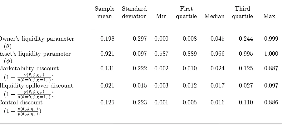
Panel A of Table III evaluates the quality of the model’s …t to the data. In the baseline

speci…cation (speci…cation (1)), the model estimates the average block premium to be 9.6%,

which is larger than the sample mean of 6.7%. In the extended speci…cation (speci…cation (2)),

the model gets closer, predicting an average block premium of 6.2%. Speci…cation (2) is better

at matching the fraction of discounts, but it underestimates the standard deviation of the block

premium. The model produces a correlation between actual and predicted block premiums of

about 0.11.

The two speci…cations predict similarCARmoments. Under both speci…cations, the model

underpredicts the mean and standard deviation of CAR, but gets close to matching the

frac-tion of negative CAR in the data. Despite underpredicting CAR, the model generates a

cor-relation between actual and predicted CAR of almost 0.4. The model can …t BP better than

CARbecause: (i) unlike share prices, block prices are also directly a¤ected by private bene…ts

of control, …re sale discounts and the bargaining power parameter; and, (ii) the variation in the

cash ‡ow distribution, which we estimate to be quite high, is smoothed out signi…cantly in p

by the fact that share prices are forward looking, therefore constraining the maximum possible

predicted CAR. A detailed discussion of point (ii) is provided in the Internet Appendix.

Recall from Section I that 74% of the trades with positive CAR exhibit a block premium

and that 75% of the trades with a negative CAR exhibit a block discount. In the baseline

speci…cation the corresponding numbers are 61% and 55% whereas in the extended speci…cation

the corresponding numbers are 77% and 67%. Note that speci…cation (2) performs well in

For both speci…cations, we reject the hypothesis that all of the model’s parameters are

zero (p-value of 0:00). Further, with 95% con…dence, we cannot reject the joint hypotheses

that the model is correctly speci…ed and that the moment conditions over-identify the model’s

parameters. We investigate the model …t also by inspecting the model’s ability to match the

moment conditions in the SMM estimation. TableIV reports a moment-by-moment match for

both speci…cations.

The model does a good job matching the moments that are most informative of and

: the unconditional mean of BP; the mean of BP CAR conditional on BP > CAR > 0;

the correlation of the valuation spread BP CAR with some of the proposed determinants of

liquidity conditional on BP > CAR >0; and, many of the correlations of BP and CAR with

some of the proposed determinants of liquidity shocks (the yield curve slope and its interactions

with GDP growth or market returns) and of …re sale values (target leverage relative to its

industry median, target industry’s asset speci…city). The ability to match the correlations of

BP andCARwith determinants of liquidity is consistent with the relatively low standard errors

for the associated coe¢ cients.

The model does poorly in matching the second order moments and speci…cally moments

that are related to CAR. One possible reason for this failure is the risk neutrality assumption

that eliminates all variation in risk premia. Future models should consider risk aversion and

variation in risk premia to better match the moments associated withCAR. Another possibility

for this failure is that that SMM gives these moments smaller optimal weights, as the estimation

procedure trades o¤ the matching error with the precision of the moments’measurement.

As an additional test to the …t of the model, we count the number of trades that satisfy

the condition that trading following a liquidity shock is ine¢ cient, that is, v( I) +B > v( R).

This condition is veri…ed in each speci…cation for all trades in the sample.

<INSERT TABLE III ABOUT HERE>

B. Parameter estimates

Panel B of TableIIIpresents the parameter estimates. We estimate the parameter associated

with market thinness, , to be 0:59 in speci…cation (1) and 0:43 in speci…cation (2). These

estimates are statistically signi…cant at the 1% level. Their magnitude suggests that a seller is

expected to meet a potential buyer absent a liquidity shock roughly once every two years.

In both speci…cations, the estimated incumbent’s bargaining power in the absence of a

liquidity shock is close 0.5. These point estimates are statistically signi…cantly di¤erent from

0, but not from 0.5. We take this result as additional empirical support for our model given

that there is no reason to expect buyers to have a bargaining advantage over sellers in times of

normal liquidity.

At the bottom of panel B of Table III, we present the estimates of the private bene…ts

function parameters. The estimated average private bene…ts per share in the block are 17.6%

in speci…cation (1) and 7.9% in speci…cation (2). Neither is statistically signi…cant at normal

signi…cance levels.

B.1. Cross-sectional determinants of owner’s liquidity

GDP growth has a negative and signi…cant e¤ect on . In terms of economic signi…cance,

and in both speci…cations, a one standard deviation increase inGDP growth is associated with a

decrease in of0:03. The sign of the point estimate supports the hypothesis that in expansions

agents have stronger balance sheets and are less likely to face liquidity shocks.

The coe¢ cient on Market Return is negative and has the strongest e¤ect on in terms of

economic signi…cance: one sample standard deviation increase in Market Return is associated

with a large decrease in of 0.11 in speci…cation (1) and of 0.31 in speci…cation (2). This

result is in line with that of GDP growth and suggests that periods of high market returns in

the sample are periods of increased liquidity. The e¤ect of Market Volatility is unexpectedly

negative, although not always signi…cant at the 5% level.

a statistically and economically signi…cant positive e¤ect on : The cost of funding as proxied

by theYield curve slope has positive e¤ect on , which is especially strong in speci…cation (2).

Speci…cation (2) adds the interactions between GDP growth and Market Return with the

Yield curve slope. The estimated coe¢ cients of these variables are positive and strongly

sta-tistically and economically signi…cant. These results support the hypothesis that blockholder

liquidity shocks are more likely to occur with the arrival of better alternative investment

op-portunities in expansions, together with high cost of borrowing.

B.2. Cross-sectional determinants of asset’s liquidity

The e¤ects of Target minus Industry Leverage and of Industry Speci…city on are negative

as expected, statistically signi…cant in both speci…cations in Table III, and in further tests

discussed later. In speci…cation (2), a one sample standard deviation increase in Target minus

Industry Leverage leads to a reduction in the …re sale parameter of 4 percentage points, and

one sample standard deviation increase in the speci…city of the industry’s assets is associated

with a decrease in the …re sale parameter of 2 percentage points.

While not statistically signi…cant, the Industry’s M&A Activity has a strong positive

ef-fect on …re sale prices. The sign of this estimate is consistent with the interpretation that a

large volume of M&A activity within an industry re‡ects enhanced liquidity for acquisitions

(Schlingemann, Stulz, and Walkling (2002)), although its lack of precision suggests the proxy

may be contaminated by supply e¤ects, which have the opposite sign.

Industry Market-to-Book has a positive e¤ect on …re sale prices, if not always statistically

signi…cant, implying that a given controlling block is worth more when there are more growth

options available in the industry. Finally, beyond these controls, we …nd insigni…cant e¤ects of

theTarget Volatility, or of the size of the block relative to its industry, Block-to-Industry Size.

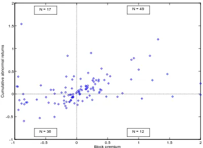
C. In-sample distributions of and

estimated average is 0.2, with a standard deviation of 0.3. This estimate suggests that on

average a blockholder is hit by a liquidity shock that forces a sale once every …ve years.8 The

table also shows that approximately 25% of the trades have an estimated of at least 24%. The

frequency of deals with extremely large may appear low relative to the42%of deals in the data

with negativeCAR. This discrepancy is explained by the following reasons. First, is an ex ante

measure of liquidity shocks computed using ex post data from each deal. A liquidity shock may

have occurred despite the low ex ante probability. Second, and more mechanically, the estimate

of is not equal to the proportion of deals with negative CAR but is a nonlinear function of

this statistic and also deal dependent. We further discuss in Section V.E the interpretation of

the size of the estimates of and of in the context of our model.

<INSERT TABLEV ABOUT HERE>

<INSERT FIGURE 3ABOUT HERE>

TableV shows that, conditional on a liquidity shock, the estimated block’s …re sale price is

on average 92% of the buyer’s block valuation, with 25% of the targets with an estimated of

less than 89%. The implied …re sale discounts are similar to estimates for other markets, that

is, to the aircraft liquidation values reported in Pulvino (1998) and to the gains from trading

on price pressure sales reported in Coval and Sta¤ord (2007). Panel (b) of Figure 3 shows the

predicted histogram of .

D. Illiquidity discounts

D.1. Marketability discount

We de…ne themarketability discount of a controlling block with respect to security bene…ts,

dM;as

dM( ) 1 v( ; ; ; :) v(0;1;1; :):

The formula makes explicit the dependence of v on , , and . It is easy to show that dM( )

dM( ) quanti…es the value of the shares in the block relative to the counterfactual scenario

where it is possible to trade at any time ( = 1) and voluntarily ( = 0). This measure of the

marketability discount di¤ers from the one in Longsta¤ (1995) because in dM it is presumed

that the blockholder remains in control, whereas in Longsta¤’s measure there is no presumption

of control.

Table V shows that the estimated average marketability discount is 13%, reaching a

max-imum of 89%. The predicted marketability discount varies with the predicted . Panel (a) of

Figure4plots the marketability discount function for every 2[0;1]. We see that, for the …rms

in the lower quartile of ;the marketability discount increases quickly, reaching 40% for just

below 20%. The estimated marketability discount is also large for blocks with intermediate …re

sale prices. However, for blocks with the highest …re sale parameter estimates, the marketability

discount is under 5% for any . Panel (b) plots the predicted distribution of the marketability

discount.

<INSERT FIGURE 4ABOUT HERE>

D.2. Illiquidity-spillover discount

We de…ne the illiquidity-spillover discount, dIS;as

dIS( ) 1 p( ; ; :) p(0;1; :):

We have that p(0; :) > p( ; :) for any >0 and that dIS _{>0. The illiquidity-spillover discount}

quanti…es the price of dispersed shares that would prevail in the absence of search costs. It is a

spillover e¤ect in that the dispersed shareholders are not hit by a liquidity shock nor experience

market thinness directly but rather through the blockholder. However, p incorporates the

possibility that control may change hands and that the value of assets will change as a result.

TableVshows that the cost of forced block turnover is important to dispersed shareholders:

we estimate an average illiquidity-spillover discount of2:1%on dispersed shares (maximum close

to 10%). This e¤ect is …ve times as large as the average quoted bid-ask spread (Bollen, Smith,

Panel (a) of Figure 5 plots the illiquidity-spillover discount against ; conditional on the

…rm’s cash ‡ow state before the trade. As the …gure shows, this discount is higher for …rms

with high cash ‡ow because these …rms have more to lose if, due to a liquidity shock, the

incumbent blockholder is forced to sell to a less e¢ cient rival. Panel (b) plots the predicted

distribution of the illiquidity-spillover discount.

<INSERT FIGURE 5ABOUT HERE>

D.3. Control discount

We de…ne the control discount from security bene…ts,dC, as

dC( ) 1 v( ; ; ; :) p( ; ; :) :

Given that v < p for any > 0, then dC _{> 0. The control discount measures the}

di¤er-ence in valuations of security bene…ts between the controlling blockholder and the dispersed

shareholders. This estimate of the control discount ignores the private bene…ts a¤orded to the

controlling shareholder. Given thatdIS is much smaller thandM, the estimated control discount

shares similar properties with the marketability discount, as displayed in TableV. As with the

marketability discount, Panel (a) of Figure 6 shows that the control discount displays high

sensitivity to the probability of a liquidity shock when the …re sale parameter is lowest (solid

line). Panel (b) of Figure 6 shows that the sample distribution of control discount is highly

skewed with many trades displaying negligible discounts.

<INSERT FIGURE 6ABOUT HERE>

The estimates of the control discount on blocks of shares in public corporations can be

applied to block valuations in the case of privately held corporations. Valuing blocks of shares

in privately held corporations is di¢ cult, as illustrated in Mandelbaum et al. v. Commissioner

of Internal Revenue (1995). As the court indicated, these di¢ culties arise from the limited

estimates of the control discount can be applied to a paired sample of comparable publicly traded

…rms with controlling blockholders to determine the block value. Using …rms with controlling

blockholders guarantees that the pricing by dispersed shareholders already incorporates the

added value of the blockholder and the illiquidity-spillover costs.

E. Interpreting discount estimates

Our modeling of search frictions has potential biases in the estimation of the parameters

and and hence potential biases in the measurement of the various discounts. Consider the

following two possible extreme alternatives. First, suppose that is a pure liquidity shock,

that is, one that does not necessarily force a sale. Then does not represent a pure …re sale

price but rather represents the blockholder’s reservation value. This reservation value is the

best outcome out of all possible ways of dealing with the liquidity shock, including when the

incumbent keeps the block but borrows against it as collateral; sells to a white knight, such

as a private-equity …rm supplying the needed liquidity; sells only a fraction of the block while

retaining control (though this is rare according to Barclay and Holderness, 1989); or, sells at a

…re sale price. While these possibilities are out of the model, we note that, since the …re sale is

the chosen alternative in our sample, then is an upper bound to the …re sale price.

Second, suppose that captures a more restrictive event: the event of a liquidity shock and

having failed to deal with it in any other way other than selling. By de…nition, this more

restrictive type of shock leads to a …re sale and then represents a pure …re sale price. In this

case, is a lower bound on a pure liquidity shock.

Consider now the impact of these two alternative interpretations of and on the

mar-ketability discount, dM_{. Becaused}M _{is decreasing in , an upper bound on the …re sale price as}

implied by the …rst scenario leads to a lower bound ondM_{. As for the second alternative, a lower}

bound on also leads to a lower bound on the marketability discount becausedM is increasing

in . In conclusion, while we may not be measuring and exactly as pure search costs, the

discount that is always a lower bound to the true marketability discount.

The illiquidity-spillover discount, dIS, is invariant to and increasing in . Hence the

esti-mation also produces a lower bound for the illiquidity-spillover discount. Finally, the control

discount dC is decreasing in , but monotonicity with respect to cannot be determined

ana-lytically. Numerically, we showed above that dC is increasing in , so that the estimated dC is

also a lower bound to the true control discount.

F. Illiquidity discounts by industry

To illustrate the cross-sectional di¤erences in the illiquidity discounts, TableVIpresents the

highest and lowest values of the discounts by 2-digit SIC code group of the target …rm. The

analysis excludes the 2-digit SIC groups with fewer than 3 observations.

Firms in the Air Transportation industry (code 45) have the highest average marketability

and control discounts. This result may be surprising given that aircraft would appear to be

assets of very low speci…city. However, Pulvino (1998) and Benmelech and Bergman (2008)

provide strong evidence that aircraft …re sales do exist, and that their liquidation values can

vary signi…cantly across airlines. The high discount estimates for this industry, which are the

result of a combination of relatively high estimates of (0.46) and relatively low estimates of

(0.81), are largely explained by high values of the high yield curve slope contemporaneous

to these trades, and the fact that the traded …rms were highly levered with respect to their

industry.

Firms in Business Services (code 73) and Electronic and Other Electrical Equipment (code

36) rank among the industries with the lowest for marketability discount. Their ranking is

explained by the fact that these industries have relatively high estimates of average , but also

high estimates of average . For Business Services, is relatively high due to a combination of a

steep yield curve and high values of theFontaine-Garcia index contemporaneous to the trades,

while is high due to low target leverage and low asset speci…city. In the case of Electronic

industry-speci…c M&A.

Industries 73 and 36 are interesting because, despite having some of the lowest marketability

discounts, they have the fourth and …fth highest illiquidity-spillover discounts, respectively.

The reason for their high illiquidity-spillover discount is the high variance of cash ‡ows in the

industry: they rank second and …fth in terms of cash ‡ow volatility, respectively. The high

cash ‡ow volatility yields a high option value associated with …nding a better blockholder to

run the …rm, but market thinness reduces the contribution of this option to share prices. For

the same reason, the …rms in Engineering, Accounting and Management Services (code 87) and

Building Contractors (code 15) rank …rst and second in terms of illiquidity-spillover discounts.

These industries have the highest and third highest estimated cash ‡ow volatilities, respectively,

among the industries in the sample.

<INSERT TABLEVI ABOUT HERE>

VI. Additional Tests

This section considers several extensions to our model. Unless noted, the results are

tabu-lated in an Internet Appendix.

A. Trading due to private bene…ts

In our model, blocks are traded due to liquidity shocks or e¢ ciency gains. In practice,

block trades may also occur due to di¤erences in private bene…ts of control, as in Burkart,

Gromb, and Panunzi (2000) or Dyck and Zingales (2004). Therefore, one important question

is whether our identi…cation of the modelled motives for trading is a¤ected by the omission of

the private bene…ts motive. For example, trades in our sample may have occurred because the

new blockholders enjoyed signi…cantly more private bene…ts than the incumbent while being

detrimental to dispersed shareholders, that is, R _< I_{. Given that those trades would also}

result in CAR < 0; we could potentially identify them incorrectly as liquidity shock-driven,