Further attempts to clarify the importance of category variability for categorisation

City, University of London Institutional Repository

Citation

:

This is the accepted version of the paper.

This version of the publication may differ from the final published

version.

Permanent repository link:

Link to published version

:

Copyright and reuse:

City Research Online aims to make research

outputs of City, University of London available to a wider audience.

Copyright and Moral Rights remain with the author(s) and/or copyright

holders. URLs from City Research Online may be freely distributed and

linked to.

1

Further attempts to clarify the importance of

category variability for categorization

Amotz Perlman, Ben-Gurion University of the Negev Ulrike Hahn, Cardiff University

Darren J. Edwards, Swansea University

Emmanuel M. Pothos, Swansea University

in press

Address correspondence to: Amotz Perlman,

Department of Psychology,

Ben-Gurion University of the Negev PO Box 653

Beer Sheva 84105 Israel

Email: [email protected]

2 Abstract

The issue of how category variability affects classification of novel instances is an important one for assessing theories of categorization, yet previous research cannot

provide a compelling conclusion. In five experiments we re-examine some of the factors which are thought to affect participant performance. In Experiments 1 and 2, participants

almost always classified the test item as belonging to the high-variability category. By contrast, in Experiment 3 we employed an alternative experimental paradigm, where the difference in variability of the two categories was less salient. In that case, participants

tended to classify a test item as belonging to the low-variability category. Two additional experiments (4 and 5) explored in detail the differences between Experiments 1, 2 on the

one hand, and 3 on the other. Some insight into the underlying psychological processes can be provided by computational models of categorization, and we focus on the continuous version of Anderson’s (1991) Rational Model, which has not been explored

before in this context. The model predicts that test instances exactly halfway between the prototypes of two categories should be classified into the more variable category,

consistent with the bulk of empirical findings. We also provided a comparison with a slightly reduced version of the Generalized Context Model (GCM) to show that its

predictions are consistent with those from the Rational Model, for our stimulus sets.

3

Inter-item variability affects behavior in a number of related areas. In categorization, the problem is how category variability influences item classification. This is an important

issue both because previous research has led to somewhat conflicting findings and because computational models of categorization make strong predictions. We discuss

some of the general literature on variability and proceed to present the relevant data from categorization, which is the focus of the present study, and corresponding computational analyses.

Variability plays a central role in studies of human inductive inference, where it has been argued that, all other things being equal, more variable, diverse evidence should

give rise to stronger inductive arguments. This diversity principle has been highlighted in the philosophy of science (see for example, Bacon, 1898; Carnap, 1950; Nagel 1939; Horwich, 1982; Howson & Urbach, 1993) and there has been considerable experimental

work examining the extent to which it is adhered to in our every day judgments by both adults (Osherson, Smith, Wilkie, Lopez & Shafir, 1990; Lopez, 1995; Lopez, Atran,

Coley, Medin & Schaffer, 1978) and children (Carey, 1985; Lopez, Gelman, Gutheil, & Smith, 1992; Gutheil & Gelman, 1997; Heit & Hahn, 2001).

The influence of diversity on inductive reasoning is likely to be related to the

influence of diversity or variability on categorization, although this link is seldom made. There is evidence that infants are sensitive to variability of categories (e.g., Mareschal,

Quinn, & French, 2002; Quinn, Eimas, & Rosenkrantz, 1993; Younger, 1985). With adults, it has been repeatedly reported that more variable observations promote broader or stronger generalizations (e.g., Rips, 1989; Stewart & Chater, 2002; Cohen, Nosofsky &

4

we call this effect the category variability effect. At the same time, there is some evidence that more variable categories are harder to acquire (e.g., Posner, Goldsmith &

Welton, 1967, Posner & Keele, 1968; Fried & Holyoak, 1984; Peterson, Meagher, Chait, & Gillie, 1973; Pothos, Edwards, & Perlman, in press). Finally, there has been some

investigation of the effects of inter item variability on memory (e.g., Homa & Vosburgh, 1976). Moreover, these various effects can be linked: Hahn, Bailey and Elvin (2005) observed effects of category variability on learning, category generalization and old/new

recognition that could be systematically related through the exemplar-based framework of the Generalized Context Model (GCM; e.g., Nosofsky, 1986, 1988). Detailed

modeling revealed that variability systematically affected sensitivity to distance in psychological space, and hence, similarity across these tasks.

Our focus is the category variability effect with adults. Closer scrutiny of the

literature reveals that, although there is plenty of empirical evidence regarding the impact of category variability on classification , results are not clear cut and

classification performance seems heavily influenced by minor, and seemingly superficial, methodological variations. Consequently, the main objective of the present paper is to identify a number of pertinent methodological manipulations and explore them further. A

secondary objective is to examine whether an influential categorization model, Anderson’s (1991) Rational Model, can provide any insight into the underlying

computational process. This model has not been explored before with respect to this issue, despite its clear relevance.

A well-known experiment by Rips (1989) provides a graphic illustration. Rips

5

diameter,” and asked them to visualize it. He next asked one group of participants if it was more similar to a pizza or a particular coin (a US currency quarter). Most of the

participants said that it was more similar to the quarter; presumably, the reason was that its diameter was closer to the diameter of the average quarter than to that of the average

pizza. He then asked a second group of participants if it was more likely to be a pizza or a quarter. Most of the participants decided pizza; seemingly because pizzas are found in a range of diameters (i.e., they are the more variable category), hence it is more likely that

they could include an exemplar with a 3-in diameter as well. By contrast, because the range of diameters in the coin category is so restricted, it seems unlikely that there would

be exemplars of the category which deviate from the typically observed extremes. An earlier report of a similar effect, but with meaningless stimuli, was made by Fried and Holyoak (1984), who showed that participants classified checkerboard examples that

were closer to the prototype (mean) of a lower variability category, as belonging to a high-variability category, which was further away.

There have been a number of extensions to the Rips’s (1989) experiment, which illustrate some subtle methodological issues. Cohen, Nosofsky, and Zaki (2001)

replicated Rips’s finding in two ways. First, they employed one-dimensional stimuli

(vertical lines), organized into a low and a high variability category, with a test instance halfway between the nearest neighbors of the two categories (in the following, test

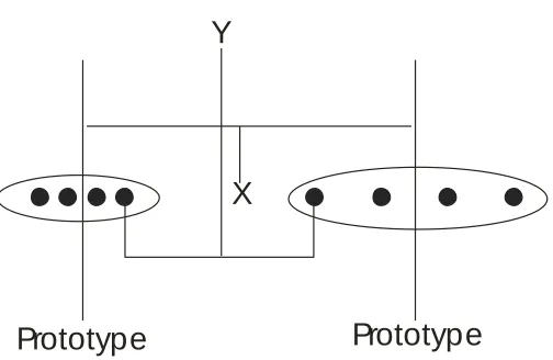
instances halfway between the nearest neighbors of two categories will be referred to as NN-halfway instances, to distinguish them from test instances located halfway between the prototypes of the two trained categories which will be referred to as P-halfway).

6

classification into the high variability category (note though that the classification rate for the high variability category was between 29.5% and 47.1%). Second, Cohen et al. also

examined stimuli which were color patches varying along two dimensions, brightness and hue (Exp. 2). In four conditions the NN-halfway test instance was always numerically

more likely to be classified into the high variability category (though these trends were not always significant).

Cohen et al. (2001) provided some interesting manipulations regarding the

importance of category variability in classification. Two methodological issues, in particular, are worth highlighting. First, in their Experiment 2, Cohen et al. defined the

low and the high variability category in such a way that, if participants were to classify the test instance in the low variability category, then there would not always be a linear category boundary separating the exemplars of the two categories. By contrast, if

participants classified the test instance in the high variability category (as most of them did), then there was always a simple linear boundary separating the exemplars of the two categories (this point is immediately obvious by inspecting Figure 4 in Cohen et al.’s

paper). There is evidence that whether a category boundary is linearly separable or not affects performance with the corresponding classification (e.g., Blair & Homa, 2001;

Ruts, Storms. & Hampton, 2004). Second, in Experiment 1, the presentation frequency of the exemplars favored the nearest neighbors of the two categories. Given the simple,

7

study the issue of category variability on classification without these methodological complications.

A related study is that of Sakamoto, Jones, and Love (2008), where participants saw test items which were NN-halfway; again, these test items were more likely to be

classified into the more variable category. In Sakamoto et al.’s study the stimuli were lines, in a way analogous to that of Cohen et al. (2002), and the training procedure was that of a standard supervised categorization experiment (participants went through several

presentations of the training stimuli, each time trying to guess their category membership and receiving corrective feedback). Sakamoto et al.’s results are consistent with those of

Cohen et al., but are somewhat at odds with earlier results from Stewart and Chater’s (2002) Experiment 1. Stewart and Chater (in their Experiment 1) also considered NN-halfway test instances, but manipulated format of presentation and the presence of a hint

regarding category variability. When Stewart and Chater employed a sequential mode of stimulus presentation (in their Experiment 1), the probability of classification into the

high variability category (without a corresponding hint) was only .25 (it was .37 with the hint). However, with simultaneous presentation of all the stimuli, this probability rose to .51 without a hint to participants that one category was more variable and .74 with such a

hint. Thus, when it comes to sequential presentation of the stimuli, and NN-halfway test instances, there is some conflict in the literature.

Overall, more recent research has somewhat emphasized NN-halfway test instances. While there are important theoretical reasons for studying NN-halfway test instances, it is worth noting that an NN-halfway item will actually be closer to the

8

the prototypes of two categories (a P-halfway item), as illustrated in Figure 1. Indeed, Cohen et al. (2001) found that a slightly reduced version of the GCM could not account

for the bias to classify NN-halfway instances into the more variable category. But, it is also theoretically pertinent to study P-halfway instances (cf. Hahn et al., 2005). One

reason is that the nearest neighbors between two categories may not be as important an aspect of category representation as, by contrast, the prototypes (note that in the Cohen et al., 2001, study the salience of the nearest neighbors was artificially enhanced in some

conditions, by increasing the frequency of these items). Thus, we think that the literature on category variability could be usefully extended by a focused study involving

P-halfway instances and this is what we aim to achieve with the present research (taking into account a range of relevant methodological manipulations). Notably, some work indicates that the default classification bias is to place an NN-halfway exemplar into the

high variability category (Cohen et al., 2001; Sakamoto et al., 2008), others that if

category variability is not made salient it will be classified in the low variability category

(Stewart & Chater, 2002). There are different ways in which variability can be made salient and this issue will be considered in our experiments.

Insert Figure 1

Our understanding of empirical results can be informed by computational models of categorization. Indeed, many computational models of categorization are sensitive to the underlying distributional characteristics of the categories that are learned. So, what do

9

prototype models determine the classification of novel instances only on the basis of category prototypes, they are blind to the effects of category variability (but see

Vanpaemel & Storms, 2008, for extensions of prototype models). Exemplar models are, in principle, sensitive to category variability, since category representations typically

involve information about all available exemplars. Cohen et al. (2001; see also Stewart & Chater, 2002) examined a version of the GCM with only one free parameter (the

sensitivity parameter) and showed that the model was more consistent with classification

of NN-halfway test instances into the low variability categories. But, as noted, the conclusions from this examination probably also depend on differences in relative

frequency between category exemplars and the complexity of the category boundaries. Stewart and Chater (2002) examined a ‘distributional’ approach (from Ashby &

Townsend, 1986), according to which probability distributions are used to represent

categories and these distributions are fitted using the observed stimuli (see also Fried & Holyoak, 1984). On this account classification of a new exemplar is based on the relative

likelihood of belonging to the distribution of each of the possible categories. An NN- halfway test item should typically be classified into the high variability category,

because the tight bunching of the exemplars in the low variability category means that the

test item is more standard deviations away from the mean of that category. A similar analysis has recently been reported by Hsu and Griffiths (2010), who examined the

10

Stewart and Chater’s analysis of the distributional approach and Hsu and

Griffiths’ (2010) examination of the baseline Bayesian model suggest that any

categorization model which represents categories in terms of the probability distribution of their members ought to predict that a halfway instance would be classified in the more

variable category. An important such model is Anderson’s (1991; see also Sanborn, Griffiths, & Navarro, 2010) Rational Model, which has come to be the most widely considered Bayesian model of categorization.

While one would expect an application of the Rational Model to the problem of category variability to lead to conclusions consistent with those of Stewart and Chater, it

is an important exercise to verify that this is indeed the case. Therefore, a secondary purpose of this work was to apply the continuous version of Anderson’s (1991; Anderson & Fincham, 1996) Rational Model to the problem of how category variability affects the

classification of novel stimuli. Note that the continuous version of the Rational Model (which assumes items are represented with continuous dimensions) has been examined

considerably less than the better known discrete version (which assumes that items are represented with discrete features).

The Rational Model assumes that the process of categorization is one of Bayesian

inference for novel stimuli. The key explanatory components of the Rational Model are the assumptions it makes regarding how experience is represented and employed when

categorizing novel instances. Specifically, it assumes that naïve observers base their category extensions on knowledge of the underlying category distributions (i.e., distributions of category exemplars). Thus, when a test instance is consistent with a

11

Model clearly predicts that classification would favor the more variable category. Thus, the issue of whether participants are sensitive to category variability or not bears on

whether participants can be assumed to encode distributional information from the observed instances and employ it for classification in the way prescribed by the Rational

Model.

More generally, examination of the Rational Model adds to the effort of

understanding cognitive process within formal probabilistic frameworks (e.g., Busemeyer

et al., 2011; Griffiths et al., 2010; Oaksford & Chater, 2007; Tenenbaum et al., 2006; Tenenbaum et al., 2011). Finally, it is worth noting that there are other categorization

models which could be applied to the category variability issue, such as the simplicity model (Pothos & Chater, 2002) or SUSTAIN (Love et al., 2004). Our choice to study the Rational Model relates primarily to the fact that, as we shall see, this model provides a

particularly clear intuition as to why category variability should matter.

The continuous version of the Rational Model

Anderson’s (1991) Rational Model is an incremental, Bayesian model of unsupervised

categorization. It assigns a new stimulus with feature structure F to whichever category k

makes F most probable. For example, a new object that looks like a ‘cat’ would be

assigned to the category of cats, since the feature structure of the object is most probable given this category membership. Specifically, the probability of classification of a novel

instance into category k is given by the productP(k)P(F|k).

cn c cn k P k    ) 1 ( ) ( ,

12

classified stimuli, and c is the coupling parameter. The coupling parameter determines how likely it is that a new instance will be assigned to a new category. Thus, c indirectly

determines the number of categories that the Rational Model will produce for a stimulus set.

The probability that the new object comes from a new category is given by

cn c c P     ) 1 ( 1 ) 0

( . P(F|k)is computed as



i x k

f ( | ), where i indexes the different

dimensions of variation of the stimuli and x indicates the different values dimension i can

take. That is, f_i(x|k) is the probability of displaying value x on dimension i in category

k, and is approximated by _a( _i, _i 1 1/ _i) i

t     , which is the t distribution with ai degrees

of freedom. _iand_i2are given by

n y n   0 0 0    and n y n n s n       0 2 0 0 0 2 2 0

0 ( 1) ( )

      ,

respectively, whereby _i ₀ n, _i ₀ n, n is the number of observations in

category k, y is their mean, and s2 is their variance. Finally, ₀ 1₀, ₀ is the

halfway point of the range of all instances and ₀ is the square of a quarter of the range.

This particular form for the Rational Model deviates very slightly from that in the original Anderson (1991) paper, but the above specification was guided by John

Anderson (personal communication; see also Pothos & Bailey, 2009, and Pothos, 2007,

which employed the Rational Model as stated above).

The account of the category variability effect given by the Rational Model can be

13

than the items of the other category. Suppose next that a novel exemplar halfway between the prototypes (means) of each of the two categories is presented; participants would be

asked to classify this novel exemplar in one category or the other. Deriving predictions regarding the classification of the intermediate item from the Rational Model is

straightforward. The model assumes that stimuli are presented sequentially and in the typical application of the model stimuli cannot be pre-assigned a classification. However, when there are two well-separated categories, the Rational Model will typically discover

them, regardless of order of presentation of the stimuli. Therefore, in order to derive a prediction for the critical intermediate item, we can first present to the Rational Model

the exemplars from the two categories, so that it can discover the two (intended)

categories, and subsequently present the intermediate item. Then, the classification of the critical test instance can be examined by presenting it last.

As noted, the standard version of the Rational Model, as proposed by Anderson (1991) and applied by us, has one free parameter, c, the coupling parameter. Lower

values of the coupling parameter make it less likely that dissimilar stimuli will be included in the same cluster and vice versa. The typical value of the coupling parameter is 0.5 and a typical range of exploring the coupling parameter, where relevant, would be

between values close to 0 and 1. We explored predictions of the Rational Model regarding category variability across a range of values of the coupling parameter. The

predictions of the Rational Model most relevant to our empirical situation correspond to values of the coupling parameter which lead to the intended classification. However, it is worth exploring the behavior of the model across several values of the coupling

14

more variable category. The input to the rational model was the stimulus coordinates for Experiment 1, as shown in Table 1a.

As expected, when the coupling parameter was very low all (or most) stimuli were assigned into separate categories (c=0.1 and c=0.2). Conversely, when the coupling

parameter was high all items were included in a single category (c=1). For c=0.3, 0.4, four separate groups were produced. Even though in these cases the halfway instance was classified into the low variability category, the low variability category was the largest

one as well: the Rational Model has a bias favoring classification into larger categories

(recall, Prob(category) ∝ nk, the number of items classified into the category so far). In

any case, as noted, all these results are not relevant for our empirical situation, since the

intended two-cluster classification was basically indicated to participants. For c= 0.5, 0.6, 0.7, 0.8, 0.9, the Rational Model predicted the intended two-cluster partition of the

stimuli. In all these cases, the critical test instance was classified into the more variable category. Thus, the Rational Model makes a robust prediction that a test instance halfway between two category prototypes should be assigned into the more variable category.

This situation is unchanged if one considers a category of low variability (instead of zero variability) and a category of high variability (e.g., as in Experiment 3). Overall, as long

as there are no large differences in category size, the Rational Model will predict that a P-halfway test instance will be classified into the more variable category.

It can be demonstrated intuitively why the rational model makes the prediction it

does. Figure 2 shows two normal distributions with a straight line halfway between the means (prototypes) of the two distributions. This situation corresponds to the stimulus

15

variability category structure has zero variability). The Rational Model works by examining how likely a new instance is, given membership into different candidate

categories. A new instance is likely to be a member of a category if it is consistent with the distributional properties of the category. Clearly, in the figure below, the instance is

much more likely given the left (more variable) category, than the right (see also Hsu & Griffiths, 2010, and Stewart and Chater, 2002). This simple, but compelling, intuition is the basis for the classification predictions from the Rational Model (for a related

illustration see Mareschal et al., 2002; for other examinations of the Rational Model, see Pothos, 2007, Pothos & Bailey, 2009, or Sanborn et al., 2010). In fact, the situation is

entirely analogous to that in standard independent samples t-tests for comparing two means.

Note that we have chosen to examine the Rational Model in an idealized situation,

without reference to participant data. We chose this approach mainly for two reasons. First, because in this way we can explore the generic model biases regarding variability

(that is, in the absence of complications which may arise from fits to noisy participant data). Second, because the standard version of the Rational Model allows relatively little flexibility in terms of particular fits anyway (the only parameter which can be

manipulated is the coupling parameter). Overall, the main relevant insight regarding the psychology of categorization from the Rational Model is that a bias to classify into the

more variable category can arise if participants encode the distributional properties of the encountered instances and utilize them in a Bayesian scheme for the classification of new instances. It is worth stressing that the assumption that the categorization process

16

contrasts with other influential approaches for categorization (e.g., prototype theory). Finally, the prediction regarding category variability from the Rational Model is robust,

that is there do not seem to be circumstances that lead to the reversal of the prediction (unless there are major differences in the relative size of the categories).

Insert Figure 2

Experiment 1

The first experiment was a basic test of the Rational Model prediction regarding category variability. In other words, we examined the prediction that a P-halfway test object will be classified as belonging to the high variability category. The procedure was designed to

make any differences in category variability as salient as possible, as this appears to make it more likely that a critical exemplar (either halfway between the prototypes or halfway

between the nearest neighbors) would be classified into the more variable category. This has been highlighted in at least three studies. For example, Smith and Sloman (1994), in an attempt to replicate Rips’s finding, reported that participants were more likely to

classify an NN-halfway critical instance in the high variability category if they could be shown (through their verbal protocols) to be aware that one category was indeed more

variable. Stewart and Chater (2002; Experiment 1) observed higher classification of an NN-halfway test instance into the more variable category if participants were told, during training, that one of the two categories was more variable. Finally, Sakamoto et al. (2008)

17

look more variable and so favored it regarding the classification of an NN-halfway critical instance.

We adopted a novel approach to the problem of making category variability salient. Rather than presenting to participants stimuli, we showed them a table with the

actual dimension values out of which the stimuli were meant to be constructed. In this way, participants could directly see the variability in each category (all participants were students in a psychology department, and so would have had some experience with

processing tables of numbers of this sort). Such an approach avoids a number of potentially tricky issues associated with previous studies. First, there would be no

problem of having to establish whether the way participants represent the stimuli is the same way as the one assumed by the experimenter (e.g., see Cohen et al., 2001). The numbers presented to participants are the exact numbers used in the examinations of the

Rational Model. Second, there are no issues arising from how well participants represent the differences between stimuli. Clearly, if participants fail to accurately perceive or

represent stimulus differences, there is no point asking about whether category variability can affect classification (cf. Smith & Sloman, 1994). Third, it might be the case that an intuition about variability may be more difficult to ascertain with a small number of

perceptual stimuli as opposed to a small set of numbers.

Regarding its other details, this experiment examined a P-halfway critical

18

simple linear ones (contrast with Cohen et al., 2001). In this way, we wanted to avoid any complications arising from category boundaries varying in complexity.

Methods

Participants

Participants were Swansea University undergraduate students, who volunteered to take part in the study. Twenty two participants were presented with Table 1 (a or b).

Procedure and stimuli

Participants were presented with the flowing instructions:

“A scientist in the Amazon discovered two types of spiders. The spiders are different in

terms of length of bodies and length of legs. Nine spiders that belong to each of the two groups (S1 group and S2 group) are presented in one table as follows:” At that point,

participants were shown either Table 1a or Table 1b, without the test item of course. The ‘a’ and ‘b’ versions of Table 1 correspond to whether the low variability category

was called S1 or S2. We also counterbalanced whether the prototype of the low variability category was ‘larger’ than the prototype of the high variability category; in

Tables 1a, 1b the prototype of the low variability category was smaller, but we also had an alternative set of materials in which it was larger. Participants were subsequently asked the following questions: “In what group is there more variability between the

spiders? 1. The S1 group or 2. The S2 group. A spider with 5 millimeters body and 5

millimeters legs is from: 1. The S1 group or 2. The S2 group.”

As can be seen in Table 1, the low variability category consisted of repeating the same item several times, that is, it had zero variability. This was done as an additional

19

salient. Moreover, the test instance was always exactly halfway between the prototypes of the two categories.

Insert Table 1

All materials were presented to participants as printed sheets of paper, and participants indicated their answers by circling the appropriate options. The experiment

lasted approximately five minutes.

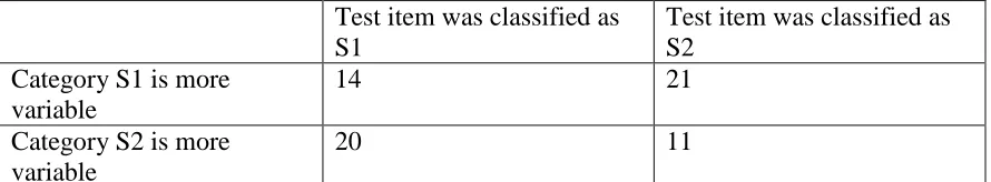
Results

All of the participants answered the first question correctly; the first question was meant to both increase the salience of category variability differences and to ensure that

participants were attending to the task. As can be seen in Table 2, participants almost

always classified the target item as belonging to the high-variability group, consistent with the prediction of the Rational Model. This can be examined statistically in two ways.

First, we can assume that factors other than category variability determine classification into the S1 or S2 category. In such a case, we would expect that classification of the test instance into the two categories will be the same, regardless of whether S1 is the more

variable category or not. Thus, we can compare the frequency of classifications across the two conditions (S1 is the more variable category vs. S2 is the more variable category),

with a chi-square test; this was found to be highly significant (Chi-square (1) = 8.82, p < .05). Second, we can examine the probability of classifying into the more variable category (regardless of whether this is S1 or S2), against a null hypothesis of chance

20

not consider classification into S1 vs. S2 as the main dependent variable, but rather classification into the more variable vs. less variable category as the main dependent

variable. A binomial distribution can be used to compute the probability of how likely it is to obtain k classifications into the more variable category, out of n, assuming an equal

probability of classifying into the more and less variable categories. This probability was

p=.001, so the null hypothesis that there is an equal classification probability into the less and more variable categories can be rejected. In other words, when S1 was the high

variability category, the test instance tended to be classified to S1 and when S2 was the high variability category, the test instance tended to be classified to S2.

Insert Table 2

Experiment 2

In Experiment 1 we found that participants classified a test instance halfway between the prototypes of a low and a high variability category to the more variable category.

However, no actual stimuli were presented. Such a manipulation was considered worth exploring in that it provided the closest possible match between the stimuli participants saw (the numbers in Table 1) and the input to Anderson’s (1991) Rational Model. In

Experiment 2, we adopted a more standard procedure, so as to examine the generality of the findings from Experiment 1. Half of the participants received only verbal descriptions

of the categories (that is, participants would see Tables 1a and 1b, as in Experiment 1), without any actual stimuli, and the other half received both the verbal descriptions and a set of actual objects (which were schematic spider-like forms).

21

Participants

The population sample consisted of 109 participants, Swansea University undergraduates,

who volunteered to take part in the study. Of these, 59 were presented with both the actual object and a verbal description and 54 participants were presented with only the

verbal description.

Procedure and stimuli

Stimuli were constructed on the basis of the values on Tables 1a and 1b which looked

like spider-like schematic drawings (Figure 3; note that there was a second set of stimuli corresponding to the counterbalancing of the values in Table 1, as discussed for

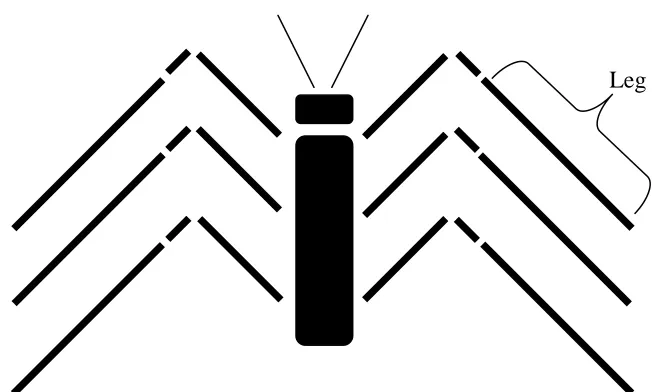
Experiment 1). The length of the legs and the length of the bodies corresponded to number of body parts and leg parts in the drawings. For example, in Figure 3 the spider on the left has four body segments (parts) and six leg segments. Additionally, together

with each spider stimulus, the number of leg and body parts were presented verbally as well. For example, the spider on the right of Figure 3 was presented with the label “2 body parts and 4 legs parts”. All of the stimuli in a group (S1 or S2) were presented on

the same sheet of paper.

Insert Figure 3

Participants received their instructions printed on an A4 sheet of paper. In the first condition, participants were presented with both the physical stimuli and the

corresponding verbal labels. Once participants indicated that they had read and

22

with the actual stimuli and their verbal descriptions and then with a third sheet (the stimuli in the S2 group; in all cases, the intended classifications were indicated). Note

that the physical size of the stimuli was such that all the stimuli in each group could fit onto a single A4 sheet. The question regarding category variability and the classification

of the item were asked in a final sheet, as has been the case in Experiment 1. The second condition was identical, but for the fact that participants saw only the verbal descriptions of the stimuli (this applies to the test stimulus as well).

Results

As can be seen in Table 3, participants who were presented with objects and verbal descriptions, were more likely to classify the intermediate item in the high variability category (Chi-square (1) = 13.665, p < .01; Binomial probability of chance classification

was found to be .0002). Accordingly, when S1 was the high variability category, participants tended to classify the test item as belonging to that S1 group and when S2

was the high variability category, participants tended to classify the test item as belonging to the S2 group. Similar results were found for participants who were presented only with the linguistic descriptions, so that, as shown in Table 3, participants were more likely to

classify the intermediate item in the high variability category (Chi-square (1)= 21.47, p < .01; Binomial probability of chance classification < .00005).

23

In Table 4 we examine the effect of presenting the actual physical stimuli. It is clear that this manipulation had very little effect and that participants always preferred to

classify the test item in the category that was more variable (Chi-square(1) = 1.18, p > .1). In other words, participants’ classification preferences were the same regardless of

whether training items were presented only verbally or with verbal descriptions combined with actual pictures of the stimuli. The conclusion from both Experiments 1 and 2 is that when the variability of a category is made salient, participants classify a test stimulus

halfway between the category prototypes in the more variable category, consistently with the predictions from the Rational Model.

Insert Table 4

Experiment 3

A key aspect in the procedure for Experiments 1 and 2 was that category variability was

made salient in a number of ways (the stimuli were shown concurrently and were

composed of segments which made stimulus differences obvious, participants were asked a question regarding category variability, and there was zero variability in one category).

In Experiment 3, we investigated a design analogous to that of Experiments 1 and 2, but where category variability was less salient. This was achieved with the use of somewhat

different stimuli (they were not composed of segments), dropping the question in the test phase relating to category variability, and using a sequential presentation procedure.

As discussed, previous, related research which employed a sequential stimulus

24

observed that an NN-halfway critical instance was more likely to be classified into the high variability category. By contrast, Stewart and Chater (2002) did not observe

classification into the high variability category with a sequential presentation; such a result was obtained only when the stimuli were presented concurrently (as in our

Experiment 2). Note, however, that all these studies employed a fairly extensive supervised categorization procedure. With this experiment, we were interested in categories which would be highly intuitive, so that a single presentation of the stimuli

would (or should) readily enable participants to understand them. This is a significant consideration in this context, because the Rational Model is a model of unsupervised

categorization, so that it cannot learn categories on the basis of feedback. Thus, the natural application of the Rational Model would be such that the intended categories are spontaneously recognized.

Finally, it is worth confirming the predictions of the Rational Model for the Experiment 3 stimuli (Table 5). For c=0.1 all items were assigned to their own clusters,

for c=1 all items were assigned to the same group. For c=0.2, 0.3, 0.4, 0.5, 0.6, 0.7, between five and three clusters were produced and in all cases the P-halfway instance was individually classified. For c=0.8, 0.9 the intended two-cluster classification was

produced and in both cases the P-halfway critical test instance was assigned to the more variable category. In other words, the Rational Model’s prediction is unchanged: the

model still predicts classification of a novel instance into the high variability category.

Methods

25

Participants were 66 Swansea undergraduates University students, who volunteered to take part in the study.

Stimuli

Stimuli were spider-like schematic drawings, analogous, but not identical, to the ones

used in Experiment 2 (see Figure 4). The length of the legs and the length of the bodies were mapped to the values in Tables 5 by assuming a Weber fraction of about 8%; such a Weber fraction is a reasonable estimate for our stimulus dimensions, since they

effectively correspond to lengths (e.g., Morgan, 2005). Moreover, as in other experiments, we counterbalanced whether the low variability category consisted of ‘small’ or ‘large’ stimuli. These considerations increase our confidence that the assumed

representation was the actual psychological one, though we did not carry out a more detailed examination of this issue (as, e.g., Cohen et al., 2001). The range of actual

lengths for both legs and bodies was the same, and it was 0 mm (when there was no body or legs) to 76.1 mm. The smallest actual length (when it was 1) of a body or leg was 20

mm. In this experiment, each stimulus was printed individually onto a sheet of paper, which was cropped to be as large as the stimulus; stimuli were subsequently laminated. Finally, in this experiment, we created two new low/ high variability categories, as seen

in Table 5. Table 5 corresponds to stimuli such that the low variability category

corresponds to low exemplars with generally low physical values and the high variability

category corresponds to exemplars with high physical values. Another set of stimuli was created by reversing the correspondence between physical values and category

26

variability category was ‘larger’ or smaller than the prototype of the high variability

category. In all cases, the test item was a P-halfway item..

Insert Figure 4

Procedure

Participants were first told that they would be presented with two groups of objects and

that the objects differed in terms of the length of the bodies and the length of the legs; two examples of possible objects were then shown to illustrate the critical dimensions. They were also told that each of the two groups had eight members. The experimenter

then started showing to participants the members of each group one by one. Each stimulus was printed on a laminated card and the stimulus order was the same as that on

Table 5 (a or b; likewise for the alternative set of values, corresponding to the

counterbalancing mentioned above). Once a stimulus had been shown, it was taken away. Finally, participants were told that they would have to decide to which group they wanted

to assign a test stimulus they were about to see. Following the question, the test stimulus was presented and participants indicated their response orally to the experimenter.

Insert Table 5

Results

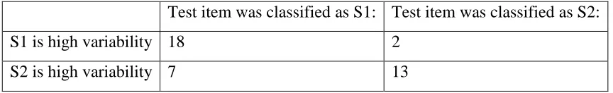
As can be seen in Table 6, participants tended to classify the target item as belonging to

27

participants tended to classify the test item as belonging to category S2, and likewise for category S2.

Insert Table 6

Experiment 4

Experiment 1, 2, and 3 provide conflicting intuitions regarding whether classification into

the more variable category is always favored or not. It appears that classification into the more variable category has to do with the extent to which differences in category

variability are made salient or not. In Experiment 3, although the two categories did differ in relative variability, there were several manipulations which were introduced to

undermine the ability of participants to perceive the relative variability of the two

categories. Specifically, in Experiment 3 the low variability category did not have zero variability, the question about variability (which was meant to function as a hint that the

two categories differed in variability) was not included, and, finally, the stimuli were sequentially presented and were not made of individual segments (in Experiments 1, 2 the stimuli were made of individual segments, so as to make any differences between

different stimuli more salient). Under such conditions, there was a preference to classify the P-halfway instance into the less variable category.

We would like to understand in more detail the factors which contribute to the perception of a difference in category variability. In Experiment 4, we employed stimuli identical to those of Experiment 2 (spider-like images, composed of segments). The low

28

But the stimuli in Experiment 4 were presented sequentially, instead of concurrently on a single sheet of paper (as in other experiments, participants were told the intended

categories). Thus, there was a single difference between Experiment 2 and Experiment 4, namely that in the latter experiment the stimuli were presented sequentially. Sequential

presentation is one of the factors which has been highlighted in previous research as encouraging classification into the less variable category (Stewart & Chater, 2002). Indeed, in Experiment 3, which employed sequential presentation, there was a bias to

classify in the less variable category. Thus, with Experiment 4 we try to isolate the

importance of sequential vs. concurrent presentation regarding the bias to classify into the

more variable category.

Methods

We recruited 40 experimentally naïve participants from the undergraduate population of

the Ben-Gurion University. The stimuli were identical to those of Experiment 2. The procedure was identical to that of Experiment 3, that is, each stimulus (with its intended

category label) was individually presented to participants. As this experiment was run in Israel, all materials were translated in Hebrew.

Results

As can be seen in Table 7, participants tended to classify the target item as belonging to the more variable group (Chi-square (1) = 12.91, p < .05; Binomial probability of chance

29

concurrent to sequential, is in itself insufficient to overcome the bias to classify a P- halfway test item into the more variable category.

Insert Table 7

Experiment 5

In Experiments 1, 2 and Experiment 3 we observed a bias for classification into the more and less variable categories respectively, but Experiments 1, 2 differed from Experiment

3 in several ways. Experiment 4 rules out one of the possible relevant differences between Experiments 1, 2 and Experiment 3. Namely, Experiment 4 showed that even

with a sequential presentation it is possible to obtain the bias for classification into the more variable category. However, Experiment 4 still differs from Experiment 3 in several ways. In Experiment 4, the less variable category still had zero variability (in Experiment

3 it did not), the stimuli were composed of segments (in Experiment 3 they did not), and the question about variability was included (in Experiment 3 it did not). Thus, there are

several factors which might be contributing to overcome the bias for classification into the more variable category in Experiment 3.

Experiment 5 was designed to examine another one of these factors, specifically

the question (hint) about variability. Previous researchers had noted that providing a hint regarding the difference in variability between the two categories increased classification

of an NN-halfway test item into the more variable category (Stewart & Chater, 2002; see also Smith & Sloman, 1994; Sakamoto et al., 2008). In the present series of experiments, such a hint had the form of asking participants which category was more variable. Is this

30

variable category? Experiment 5 was identical to Experiment 4, but the question about category variability was dropped. (Recall, Experiment 4 was identical to Experiment 2,

but for the fact that in Experiment 4 the stimuli were sequentially presented, while in Experiment 2 presentation was concurrent.)

Methods

We recruited 40 experimentally naïve participants from the undergraduate population of the Ben-Gurion University. The stimuli and procedure were identical to those of

Experiment 4, but for the fact that the question about category variability was not included. As this experiment was run in Israel, all materials were translated in Hebrew.

Results

As can be seen in Table 8, participants tended to classify the target item as belonging to the more variable group but the results were not significant (Chi-square (1) = 1.76, p > .1;

Binomial probability of chance classification = 0.057). In other words, the results of Experiment 5 are exactly in between the results of Experiment 1, 2, and 4 and the results

of Experiment 3. Experiment 5 shows that not including the question about category variability is an important factor in whether participants classify into the more variable category or not.

Insert Table 8

General discussion

The empirical objective of this study was to reassess some of the conclusions regarding the impact of category variability on the classification of instances halfway between two

31

chose to focus on test instances halfway between prototypes (P-halfway instances), because prototypes are undeniably important characteristics of a category. By contrast,

some researchers have considered test instances halfway between the nearest neighbors of two categories (NN-halfway instances). We were reluctant to adopt this alternative

approach. The nearest neighbors between two categories would be the least typical members of the categories (in statistical terms, they might be outliers, though whether they are outliers or not would depend on the overall distributional characteristics of the

relevant categories). Therefore, their importance in the classification of new instances is debatable. Even though standard exemplar models do not specifically weigh some

category members more than others, whether this is indeed the case or not has yet to come under close empirical scrutiny.

Our experiments were designed to incorporate a number of factors which may

impact on classification into the more variable category. These factors were: the form of the stimuli (whether they were made of segments or not; in the former case, stimulus

differences would be more salient), stimulus presentation format (concurrent vs. sequential), the variability of the low variability category (if it is zero, then presumably the difference in variability between the low and the high variability categories is more

obvious), and a question about which category was more variable (this was meant to encourage participants to appreciate that there was a difference in the variabilities of the

two categories). Experiments 1 and 2 were designed to have in place several of the factors thought to encourage participants to appreciate the difference in the variability of the two categories. In these cases, we found that a test instance halfway between the two

32

Experiment 3 most of these factors were eliminated, leading to a preference for classifying the halfway test instance as belonging to the low variability category.

Experiments 4 and 5 were designed to explore in more detail the conditions which make it more likely that a P-halfway test instance would be classified into the more

variable category. Experiment 4 was identical to Experiment 2, but for the fact that the stimuli were presented sequentially instead of concurrently. We found that in Experiment 4 classification into the more variable category was still favored. Experiment 5 was

identical to Experiment 4 but for the fact that the question about variability was dropped. In that case the results showed no significant bias to classify in the low or high variability

category. Thus, Experiments 4 and 5 provide a graded picture for how the pattern of results in Experiment 2 eventually lead to the pattern of results in Experiment 3 and highlight the relative importance of the corresponding experiment characteristics. Table 9

provides a summary of the experiments and key results.

Insert Table 9

This pattern of results is partly consistent with previous relevant research. For

example, as with previous researchers, we concluded that in general when the difference in variability between two categories was made salient, the test instance was more likely

to be classified in the more variable category (Sakamoto et al., 2008; Smith & Sloman, 1994; Stewart & Chater, 2002). We also confirmed the importance of a hint regarding the difference in variability between the two categories (Stewart & Chater, 2002). But, we

33

in undermining the assumed bias to classify a halfway instance into the more variable category (Stewart & Chater, 2002).

It is worth providing a brief consideration of why we observed a bias for

classification into the less variable category in Experiment 3, though a full examination

of this issue is beyond the scope of our work. One possibility is that the processing of non-identical stimuli when presented sequentially does not lead to memory traces that are stable enough and detailed enough, for participants to get an accurate sense of differences

in category variability, or, indeed an accurate sense of the categories themselves. Under such circumstances, maybe the low variability category is favored for the classification of

the test instance simply because it is learned better (or, because for the low variability category participants find it easier to come up with a heuristic rule to represent it; cf. Ashby et al., 1998). That is, classification results in Experiment 3 may depend not on

which category is more or less variable, but rather on which category had been better acquired.

Experiment 3 was actually the only experiment in which the low category variability had non-zero variability. Is this a critical factor in terms of the preference for the low variability category we observed in this experiment? We think this is unlikely.

First, there is no theory as to why zero variability would be qualitatively different from low, but non-zero variability. Second, even given the fact that the stimuli in the low

variability category were identical, it is arguable as to whether the psychological

representations of the stimuli were exactly identical as well. Participants probably felt the stimuli were nearly the same, but to establish exact identity closer scrutiny would be

34

our tentative suggestion is that a difference between zero and low variability is only one of the factors making a difference in the variability of categories salient, and does not

impact on participant performance in another way.

To sum up, our results add support for the view that classification of a P-halfway

test instance is more likely to be in a high variability category, as opposed to a low variability one, as long as the difference in category variability is salient. Our results complement the considerable related literature on NN-halfway test instances and

consolidate some of the intuitions regarding when it is more likely for classification into the more variable category to occur.

We also explored the predictions from the Rational Model of categorization (Anderson, 1991; Sanborn, Griffiths, & Navarro, 2010), which is the predominant Bayesian model of categorization. We implemented the continuous version of the

Rational Model, which clearly predicts that a P-halfway test item will be classified into the more variable category. It is worth noting that this prediction holds across a wide

range of manipulations of its main parameter, the coupling parameter. Our results are mostly consistent with the Rational Model, since participants did indeed typically classify the P-halfway test instance into the more variable category. This suggests that perhaps the

bias for classification of P-halfway instances into the more variable category could arise because of a representation of the distributional properties of category exemplars and an

assessment of new instances in terms of such distributional properties. However, the Rational Model cannot explain, for example, the results in Experiment 3, whereby participants favored classification into the less variable category. We can speculate as to

35

3 result. The most obvious culprit is the assumption regarding the input to the model. As noted above, perhaps the sequential presentation of the stimuli did not allow participants

to develop the intended categories or appreciate the differences in the variability of categories (note that the Rational Model, and other related computational models, have

no straightforward way to formalize this idea). However, as also noted, we cannot preclude the possibility that there are restrictions in the applicability of the psychological processes assumed by the Rational Model and that, in some cases, alternative

categorization modes are engaged (cf. Ashby et al., 1998).

Nosofsky (1991) argued that certain versions of exemplar theory are consistent

with the predictions of the Rational Model (for his argument he employed a precursor to the GCM). So, one would expect that predictions from the GCM would (typically) converge with predictions from the Rational Model. But, as noted, Cohen et al. (2001)

found that a slightly reduced version of the GCM was not consistent with a bias for classification into the more variable category, at least for NN-halfway instances. What is

the situation for P-halfway instances? Rather than fit the GCM to participant data, as has been the case for our examination of the Rational Model, we believe a more informative analysis of the model’s properties would be provided by an idealized situation whereby

the P-halfway instance (e.g., in Table 1a) is assigned with 100% probability to either the low or the high variability category—an examination of the model’s sum of squares (SoS) error for the alternative classifications will reveal the model’s bias regarding more

vs. less variable categories.

We explored the full version of the GCM, subject only to the requirement that the

36

parameter was constrained to be between 1 and 2 (since the exponential and Gaussian similarity functions have been the only ones which have been supported in the literature)

and the Minkowski power metric parameter was constrained to be between 1 and 2 as well (since the City block and Euclidean metrics are likewise the only ones which have

been advocated as psychologically relevant). Attentional weights were allowed to vary freely between 0 and 1, subject to a constraint that they sum to 1. Finally, the upper limit of the sensitivity parameter was manipulated (with perfectly linear categories and perfect

classification probabilities, the GCM will nearly always favor the max allowed value of the sensitivity parameter; Pothos & Bailey, 2009). For the Table 1a stimuli, we examined

upper limits for the sensitivity parameter of 100, 50, 10, and 5, 1, and 0.5, and in all cases the SoS error was higher when the P-halfway instance was assigned to the low variability category than when it was assigned to the high variability category. Analogous results

were obtained for the Table 3 stimuli.

These results show that for our stimulus sets the GCM favors classification of a

P-halfway test instance into the more variable category. Intuitively, the GCM favors classification into a more variable category for P-halfway instances because of its

exponentially decaying similarity function. A P-halfway test instance will be closer to the

nearest neighbor from the high variability category, than the low variability one.

Moreover, an exponentially decaying similarity function means that classification of the

test instance will be more heavily influenced by near instances, while the influence of instances further away will rapidly (exponentially) diminish. The consistency of the Rational Model and the GCM in relation to P-halfway instances highlights the

37

In conclusion, we presented several new experiments regarding classification biases for a test instance halfway between the prototypes of two categories and examined

the predictions from two important categorization models. The emerging conclusion is that there is a bias for classification into the more variable category, although this bias

38

Acknowledgements

This research was partly supported by ESRC grant R000222655 to EMP. We would like to thank John Anderson for his help with the specification of the Rational Model.

References

Anderson, J. R. (1991). The adaptive nature of human categorization. Psychological Review, 98, 409-429.

Anderson, J. R. (1993). Rules of the Mind. Lawrence Erlbaum Associates: Hillsdale, NJ.

Anderson, J. R., & Fincham, J. M. (1996). Categorization and sensitivity to correlation. Journal of Experimental Psychology: Learning, Memory, and Cognition, 22, 259–277.

Ashby, G. F. & Townsend, J. T. (1986). Varieties of perceptual independence.

Psychological Review, 93, 154-179.

Ashby, G. F., Alfonso-Reese, L. A., Turken, A. U., & Waldron, E. M. (1998). A Neuropsychological Theory of Multiple Systems in Category Learning. Psychological Review, 105, 442-481.

Bacon, F. (1620/1898). Novum Organum. London: George Bell and Sons.

Blair, M. & Homa, D. (2001). Expanding the search for a linear separability constraint on category learning. Memory & Cognition, 29, 1153-1164.

Busemeyer, J. R., Pothos, E. M., Franco, R., & Trueblood, J. (2011). A quantum

theoretical explanation for probability judgment errors. Psychological Review, 118, 193-218.

39

Carnap, R. (1950). Logical foundations of probability. University of Chicago Press.

Cohen, A.L., Nosofsky, R.M., & Zaki, S.R. (2001). Category variability, exemplar similarity, and perceptual classification. Memory & Cognition, 29, 1165-1175.

Fried, L. S., & Holyoak, K. J. (1984). Induction of category distributions: A framework for classification learning. Journal of Experimental Psychology: Learning, Memory, and Cognition, 10, 234–257.

Griffiths, T. L., Chater, N., Kemp, C., Perfors, A., & Tenenbaum, J. B. (2010).

Probabilistic models of cognition: exploring representations and inductive biases. Trends in Cognitive Sciences, 14, 357-364.

Gutheil, G., & Gelman, S. A. (1997). Children’s use of sample size and diversity

information within basic-level categories. Journal of Experimental Child Psychology, 64, 159-174.

Hahn, U., Bailey, T. M., & Elvin, L. B. C. (2005). Effects of category diversity on learning, memory, and generalization. Memory & Cognition, 33, 289-302

Heit, E., & Hahn, U. (2001). Diversity-based reasoning in children. Cognitive Psychology, 43, 243-273.

Homa, D., & Vosburgh, R. (1976). Category breadth and the abstraction of prototypical information. Journal of Experimental Psychology: Human Learning and Memory, 2, 322-330.

40

Howson, C. & Urbach, P. (1993). Scientific reasoning: The Bayesian approach. Chicago: Open Court.

Hsu, A. S. & Griffiths, T. L. (2010). Effects of generative and discriminative learning on use of category variability. Proceedings of the 32nd Annual Conference of the Cognitive Science Society.

Lopez, A. (1995). The diversity principle in the testing of arguments. Memory & Cognition, 23, 374-382.

Lopez, A., Gelman, S. A., Gutheil, G., & Smith, E. E. (1992). The development of category-based induction. Child Development, 63, 1070-1090.

Lopez, A., Atran, S., Coley, J. D., Medin, D. L., & Smith, E. E. (1997). The tree of life: Universal and cultural features of folkbiological taxonomies and inductions. Cognitive Psychology, 32, 251-295.

Love, B. C., Medin, D. L., & Gureckis, T. M. (2004). SUSTAIN: A network model of category learning. Psychological Review, 111, 309-332.

Mareschal, D., Quinn, P. C. & French, R. M. (2002). Asymmetric interference in 3- to 4-month-olds' sequential category learning. Cognitive Science, 26, 377-389.

Medin, D. L. & Schaffer, M. M. (1978). Context Theory of Classification Learning.

Psychological Review, 85, 207-238.

Morgan, M. J. (2005). The visual computation of 2-D area by human observers. Vision Research, 45, 2564-2570.

41

Nosofsky, R. M. (1984). Choice, similarity, and the context theory of classification.

Journal of Experimental Psychology: Learning, Memory, and Cognition, 10, 104-114.

Nosofsky, R. M. (1986). Attention, similarity, and the identification categorization relationship. Journal of Experimental Psychology: General, 115, 39-57.

Nosofsky, R. M. (1988). Exemplar-based accounts of relations between classification, recognition, and typicality. Journal of Experimental Psychology: Learning, Memory, and Cognition, 14, 700-708.

Nosofsky, R. M. (1991).Relation between the rational model and the context model of categorization. Psychological Science, 2, 416-421.

Oaksford, M. & Chater, N. (2007). Bayesian rationality: The probabilistic approach to human reasoning. Oxford: Oxford University Press.

Osherson, D. N., Smith, E. E., Wilkie, O., Lopez, A., & Shafir, E. (1990). Category-based induction. Psychological Review, 97, 185-200.

Peterson, M. J., Meagher, R. B. Jr., Chait, H., & Gillie, S. (1973) The abstraction and generalization of dot patterns. Cognitive Psychology, 4, 378-398.

Posner, M. I., & Keele, S. W. (1968). On the genesis of abstract ideas. Journal of Experimental Psychology, 77, 353-363.

Posner, M. I., Goldsmith, R., & Welton, K. E. Jr. (1967) Perceived distance and the classification of distorted patterns. Journal of Experimental Psychology, 73, 28-38.

42

Pothos, E. M. & Chater, N. (2002). A Simplicity Principle in Unsupervised Human Categorization. Cognitive Science, 26, 303-343.

Pothos, E. M. & Bailey, T. M. (2009). Predicting Category Intuitiveness With the Rational Model, the Simplicity Model, and the Generalized Context Model. Journal of Experimental Psychology: Learning, Memory, and Cognition,35, 1062–1080.

Pothos, E. M., Edwards, D. J., & Perlman, A. (in press). Supervised vs. unsupervised categorization: Two sides of the same coin? Quarterly Journal of Experimental Psychology.

Quinn, P. C., Eimas, P. D., & Rosenkrantz, S. L. (1993). Evidence for representations of perceptually similar natural categories by 3-month-old and 4-month-old infants.

Perception, 22, 463-475.

Rips, L. J. (1989). Similarity, typicality, and categorization. In S. Vosniadou & A. Ortony (Eds.), Similarity and analogical reasoning (pp. 21–59). New York: Cambridge

University Press.

Ruts, W., Storms, G., & Hampton, J. (2004). Linear separability in superordinate natural language concepts. Memory & Cognition, 32, 83-95.

Sakamoto, Y., Jones, M., & Love, B. C. (2008). Putting the psychology back into psychological models: Mechanistic versus rational approaches. Memory & Cognition, 36,1057-1065.

Sanborn, A. N., Griffiths, T. L., & Navarro, D. J. (2010). Rational approximations to

43

Shepard, R. N. (1987). Toward a Universal Law of Generalization for Psychological Science. Science, 237, 1317-1323.

Smith, E. E. & Sloman, S. A. (1994). Similarity- versus rule-based categorization.

Memory & Cognition, 22, 377-386.

Stewart, N., & Chater, N. (2002). The effect of category variability in perceptual

categorization. Journal of Experimental Psychology: Learning, Memory, and Cognition, 28, 893–907.

Tenenbaum, J.B., Griffiths, T.L., & Kemp, C. (2006). Theory-based Bayesian models of inductive learning and reasoning. Trends in Cognitive Sciences, 10, 309-318.

Tenenbaum, J. B, Kemp, C., Griffiths, T. L., & Goodman, N. (2011). How to grow a mind: statistics, structure, and abstraction. Science, 331, 1279-1285.

Younger, B. A. (1985). The segregation of items into categories by ten-month-old infants. Child Development, 56, 1574-1583.

44

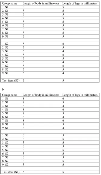
Table 1

The tables below show the test items and their dimensions, exactly as presented to participants in

Experiment 1. The test items were supposed to correspond to hypothetical spiders. Low values correspond to exemplars from the low variability category.

a.

Group name Length of body in millimeters Length of legs in millimeters

1. S1 3 5

2. S1 3 5

3. S1 3 5

4. S1 3 5

5. S1 3 5

6. S1 3 5

7. S1 3 5

8. S1 3 5

9. S1 3 5

1. S2 8 6

2. S2 7 5

3. S2 6 4

4. S2 8 6

5. S2 7 5

6. S2 6 4

7. S2 8 6

8. S2 7 5

9. S2 6 4

Test item (S2) 5 5

b.

Group name Length of body in millimeters Length of legs in millimeters

1. S1 8 6

2. S1 7 5

3. S1 6 4

4. S1 8 6

5. S1 7 5

6. S1 6 4

7. S1 8 6

8. S1 7 5

9. S1 6 4

1. S2 3 5

2. S2 3 5

3. S2 3 5

4. S2 3 5

5. S2 3 5

6. S2 3 5

7. S2 3 5

8. S2 3 5

9. S2 3 5