Transfer function characterization for HFCTs used in partial discharge detection

Transfer Function Characterization for HFCTs used in

Partial Discharge Detection

Xiao Hu, W. H. Siew, Martin D. Judd

University of Strathclyde 204 George Street Glasgow G1 1XW, UK

and

Xiaosheng Peng

State Key Laboratory of Advanced Electromagnetic Engineering and Technology School of Electrical and Electronic Engineering

Huazhong University of Science and Technology, Wuhan, China, 430074

ABSTRACT

High frequency current transformers (HFCTs) are widely employed to detect partial discharge (PD) induced currents in high voltage equipment. This paper describes measurements of the wideband transfer functions of HFCTs so that their influence on the detected pulse shape in advanced PD measurement applications can be characterized. The time-domain method based on the pulse response is a useful way to represent HFCT transfer functions as it allows numerical determination of the forward and reverse transfer functions of the sensor. However, while the method is accurate at high frequencies it can have limited resolution at low frequencies. In this paper, a composite time-domain method is presented to allow accurate characterization of the HFCT transfer functions at both low and high frequencies. The composite method was tested on two different HFCTs and the results indicate that the method can characterize their transfer functions ranging from several kHz to tens of MHz. Results are found to be in good agreement with frequency-domain measurements up to 50 MHz. Measurement procedures for using the method are summarized to facilitate further applications.

Index Terms — HF transformers, current transformers, transfer functions, time domain measurements, partial discharges.

1

INTRODUCTION

PARTIAL discharge (PD) is a localized electrical discharge that only occurs in part of the insulation between conductors [1]. PD is indicative of local defects within electrical insulation and has been recognized as an effective tool for diagnosing the insulation condition of high voltage (HV) equipment. By measuring PD, defects that may develop into faults can be found and rectified, thus helping to achieve improved operational reliability and maintenance efficiency. High frequency current transformers (HFCTs) are widely used as sensors in PD detection and monitoring systems applied to HV equipment. Their role in PD detection is to convert transient currents into corresponding voltages that can be recorded by measurement or monitoring equipment. Typical HFCTs used in PD detection applications have bandwidths of three to four decades (e.g., 10 kHz to 10 MHz) and the current levels they are designed to measure are usually much lower than the power frequency currents carried by the HV circuit [2]. Since no direct connection to a circuit under

test is required, HFCTs provide good electrical isolation of the measurement instrument. This is a major advantage of clamp-on HFCTs as it allows measurement of PD pulses with minimal disturbance to the circuit (they can often be retrofitted while plant remains in service). PD usually generates short transient current pulses that usually have a risetime in the ns range so that the bandwidth can extend up to 1 GHz [3]. The transient currents can be measured by clamping HFCTs around conductors in which they flow. In this way, HFCTs have been widely applied to detect PD in high voltage components including power cables and cable accessories, power and instrument transformers, rotating machines and switchgears [4-7]. Particularly, on-line PD testing of power cables and cable accessories takes place predominantly using HFCT sensors [8].

A typical HFCT consists of a ferrite core wound with a coil that is terminated with a load impedance that is usually 50 Ω for PD measurement [2]. The voltage output of the HFCT is proportional to the current flowing through it at a given fixed frequency. Overall, the HFCT has a frequency-dependent response that is effectively a bandpass characteristic. PD-induced

Figure 1.Structure of a HFCT with a single-turn primary carrying current Ip and a multi-turn secondary generating output voltage Uo across a resistive load Rl [2].

Figure 2. Equivalent circuit of the HFCT where Ip is primary current; Is and Us are the secondary current and voltage respectively; Np and Ns are primary and secondary turn numbers; Rs is the secondary winding resistance; Ls is the secondary leakage inductance; Cs is the parasitic secondary loading capacitance; Rl is the output load resistance; and Uo is the HFCT output voltage.

current pulses are broadband and the response of the HFCT modifies the pulse features. It can be advantageous if the HFCT’s effect on the measured PD pulses is corrected to have better resolution of the original features since advanced PD monitoring systems are increasingly moving to higher sampling rates for PD pulses, and using more detailed features of the PD pulses for the purpose of separating PD signals from noise and classification of different PD types [9,10]. To make the correction, a possible solution is to create a digital model of the HFCT response that allows its transfer function has to be accurately characterized [11]. While for commercial HFCTs, a frequency response plot should be provided, this may not be sufficient for reasons including: 1) limited frequency band that may not cover the full spectrum of the PD pulse; 2) no information on the phase response; 3) insufficient detail of the test configuration and methodology used to perform the frequency response measurement.

Approaches to characterizing the response of a HFCT can be divided into frequency-domain and time-domain methods. For the frequency-domain method, a signal source is used to feed the HFCT with a sinusoidal current that is swept over a range of frequencies and its corresponding output voltage is recorded. By dividing the voltage output by the input current at each frequency, the HFCT transfer function is obtained [12], [13]. The frequency-domain method is straightforward but tends to be less accurate at high frequencies because, as the wavelength gets shorter, the physical size of the mounting arrangement of the HFCT and test rig are no longer of insignificant dimensions compared to the wavelength. As a result, impedance mismatch effects become significant and degrade the measurement. To improve the accuracy of the frequency-domain method at high frequencies, some calibration measures were developed [14-16] but implementing them requires sophisticated equipment such as vector network analyzers which are not easily accessible. For the time-domain method, a pulse source is used to excite the HFCT and its transfer function is derived numerically using fast Fourier transform (FFT) methods applied to the output voltage and the input current waveforms [17]. The time-domain method based on the pulse response is effective at high frequencies but can have poor accuracy at low frequencies because the time length of the time-domain responses will be limited for experimental and numerical reasons. However, it is the long-time response that is related to the low frequency contents in the spectrum.

Both the time-domain and frequency-domain methods have some disadvantages. In this paper, based on the time-domain method a composite measurement scheme is devised. The scheme is simple to use and effective for characterizing HFCT transfer functions over a range of frequencies well beyond the typical 3 dB points of the HFCT (104 to 107 Hz). The objective of the proposed method is to obtain the HFCT transfer function in a form suitable for integration into a modeling framework for simulating HFCT-based PD detection in high voltage cables.

2 STRUCTURE AND EQUIVALENT CIRCUIT

OF HFCTS

A HFCT consists of a toroidal core material (usually with high permeability such as ferrite) and insulated copper wire wound on the core with a load impedance connected between its terminals. Figure 1 shows a typical diagram of a HFCT in use, which has a single-turn primary consisting of the central current-carrying conductor and multi-turn secondary. A resistive load is connected to the secondary terminals to convert the secondary current to a corresponding voltage. The turns ratio arrangement (one-turn primary and multi-turn secondary) combined with the use of a resistive load at the secondary can increase the secondary voltage while at the same time alleviating the parasitic inductance problem that becomes more apparent at higher frequencies [2].

A simplified equivalent circuit of the HFCT is shown in Figure 2. Based on the equivalent circuit and transformer theory [18] it is possible to derive a transfer function between the primary current Ip (input) and the HFCT output voltage

Uo. Firstly, the secondary voltage Us can be calculated by

dt d N

Us s





 (1) where Φ is the magnetic flux in webers passing through the magnetic core. The total magnetomotive force (MMF) in ampere-turns excited by the primary and secondary currents Ip and Is can be calculated as

s s p

pI N I

N

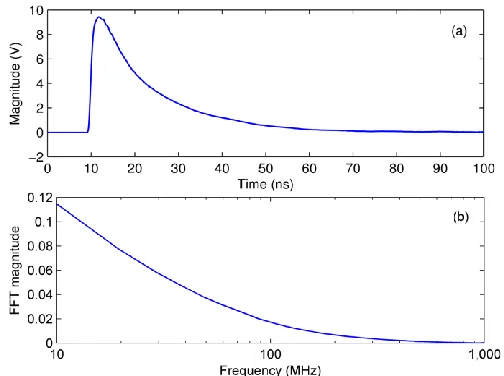
Figure 3.(a) Output waveform of the avalanche transistor pulse generator and (b) its FFT magnitude spectrum. The generated pulse typically has a risetime below 1 ns. The sampling rate used to acquire the waveform was 10 GS/s. and the resulting Φ is

c r m m m A l R R MMF







 (3)

where Rm is the magnetic core reluctance, lm is the magnetic

path length, Ac is the cross-sectional area of the magnetic

core, μ0 = 4π × 10-7 H/m is the permeability of free space and

μr is the relative permeability of the core material.

By substituting equations (2) and (3) into equation (1), the secondary voltage Us is then represented as

dt I N I N d l A N

U p p s s

m c r s s ) (

0  









where Np = 1 for the HFCT. Secondly, in the equivalent

circuit Uo can be expressed in terms of Us using Laplace

notation as s l s s l s s s l s l o R R C R R L s C L R s s U R s U       ) ( ) ( )

( ₂ (5)

By applying the Laplace transform to both sides of equation (4) and substituting into equation (5), the transfer function between Uo and Ip is finally obtained as

s l s s l s s s l p l s p o R R M C R R L s M L C R s s I R N N sM s U          ) ( ) ( ) ( ) / ( )

( ₂ (6)

where M = Ns2μ0μrAc/lm. Using equation (6) and assuming

that the HFCT component values are known, the magnitude and phase responses of the HFCT transfer function can be plotted. In practice, a reverse process is often adopted, whereby plotting the HFCT transfer function through measurement first and then a process of fitting to equation (6) is used to estimate the values of the unknown parameters.

3 TRANSFER FUNCTION

CHARACTERIZA-TION USING TIME-DOMAIN METHOD

By feeding a transient into a HFCT under test, the time-domain method requires measuring both the transient input (primary current) Ip and the HFCT output Uo waveforms, and

then the frequency-dependent transfer function TFct in V/A

(Ω) can be calculated by

] [ FFT ] [ FFT p o ct I U

TF  (7) where FFT is the fast Fourier transform. The feed arrangement for Ip is often made by terminating the transient

source with a resistance Rin. Hence, Ip can be obtained

through Ip = Uin / Rin where Uin is the voltage across Rin.

Compared to the frequency-domain method where measurement has to be carried out at each individual frequency, the time-domain method, with only one measurement, can give the complex transfer function (both magnitude and phase) at all frequencies that are generated by applying FFT to the waveforms. This makes it particularly attractive for measuring the HFCT transfer function over a wide frequency range. However, since the spectral content of

a transient source can cover a specific frequency band only, using the transient source as the input is not sufficient for characterizing the complete transfer function of HFCTs which usually have bandwidths of three to four decades of frequency.

4 COMPOSITE TIME-DOMAIN METHOD

Considering that a HFCT can have a very wide usable bandwidth, a composite time-domain measurement scheme was adopted. By using a transistor avalanche pulse generator with a sub-nanosecond risetime as the signal source, the obtained pulse response can be substituted into equation (7) to calculate the HFCT transfer function in the range of 10 MHz to 1 GHz. Similarly, by using a standard function generator to apply a positive pulse as the signal source (edge transition times in the region of 13 to 15 ns), the HFCT transfer function can be obtained in the range of 20 kHz to 1 MHz. At frequencies between 1 and 10 MHz, the HFCT transfer function is resolved using further numerical processing described later.

The lowest resolvable frequency flow of an FFT spectrum is

inversely proportional to the record length T of time-domain data [19] and can be calculated by

T flow

1

 (8) A trace of the avalanche pulse was acquired for a record length of T = 100 ns. Figure 3 shows the voltage waveform and its FFT spectrum from the spectrum's lowest resolvable frequency flow = 10 MHz. After a few hundred megahertz, the

spectrum magnitude was less than one tenth of the value at 10 MHz. The bandwidth of the oscilloscope used for the measurements was 1 GHz, which is sufficient to cover the spectral content of the pulse.

Figure 4.(a) Voltage waveform and (b) FFT spectrum of the positive pulse applied by the function generator. The rising edge has a risetime of 13 ns and the falling edge has a falltime of 15 ns. The spectrum ripple is a function of the pulse width. The sampling rate used to acquire this waveform was 500 MS/s.

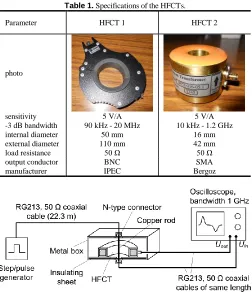
Table 1.Specifications of the HFCTs.

Parameter HFCT1 HFCT2

photo

sensitivity 5 V/A 5 V/A -3 dB bandwidth 90 kHz - 20 MHz 10 kHz - 1.2 GHz internal diameter 50 mm 16 mm external diameter 110 mm 42 mm load resistance 50 Ω 50 Ω output conductor BNC SMA manufacturer IPEC Bergoz

Figure 5.Diagram of the setup for measuring HFCT transfer functions. The HFCT is placed in the box on an insulating sheet. The input and output waveforms are recorded at the 50 Ω inputs of a wideband digital sampling oscilloscope.

rising and one falling. Compared with Figure 3b, the FFT pulse spectrum of Figure 4b contains data over a lower band of frequencies, namely 20 kHz to 1 MHz. The spectrum's lowest frequency decreased to 20 kHz because of the 50 μs record time.

The HFCT transfer function for the two bands of frequencies may be combined to produce one complete composite response. One possible solution is to have the high frequency part's minimum frequency decreased from 10 MHz to 1 MHz and the low frequency part's maximum frequency increased from 1 MHz to 10 MHz. This would make it possible to find a frequency between 1 MHz and 10 MHz where the response of the two parts come very close and thus can be made coincident at that frequency. In terms of frequency limits, the transfer function calculated using equation (7) will have its maximum and minimum frequencies defined by the parameters of the FFT input data. Therefore, in order to decrease the minimum frequency of the calculated transfer function, the number of points NFFT used in calculating FFT in equation (7) needs to be increased. This can be done by adding zero-valued samples to the end of the time-domain data to increase the length of the window T [19]. In this paper, the record of the avalanche pulse response contained 1,002 samples. Adding 15,382 zero-valued samples to the end of the record made it 16,384 samples so that the frequency resolution of the corresponding FFT spectrum can be decreased to 0.61 MHz (i.e., the extended minimum frequency of the high frequency part). For the low frequency part obtained using the positive pulse response, the FFT maximum frequency was 250 MHz which was determined by the Nyquist law and the 500 MS/s sampling rate used to acquire the data of the positive pulse response. Nevertheless, from around 1 MHz upward there was increasingly apparent noise in the calculated transfer function. This was caused by that the frequency spectrum of the positive pulse was mainly

within 1 MHz. In order to remove the noise, calculating the running median of the transfer function was implemented. It will be shown later that at frequencies < 10 MHz this approach was effective for smoothing out the noise in the low frequency part of the transfer function.

5 TIME-DOMAIN MEASUREMENT ON

HFCTS

5.1 HFCT SPECIFICATIONS

Two quite different types of HFCT have been used in the practical measurements. Their transfer functions are of interest to allow implementation of a modeling framework for simulating HFCT-based PD detection in high voltage cables. The HFCTs and their specifications are as shown in Table 1. While the sensitivities and bandwidths provided in the specifications are appropriate for the purpose of selecting HFCTs for specific applications, they do not sufficiently define the response to enable modeling of the HFCTs' effects on the PD-induced current pulse shapes. To that end, HFCT transfer functions including the phase response have to be characterized numerically through measurements.

5.2 MEASUREMENT SETUP

Figure 6.(a) positive pulse response and (b) avalanche pulse response of HFCT 1. They were obtained by using the positive pulse shown in Figure 4 and the

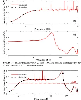
avalanche pulse shown in Figure 3 as the input respectively. _{Figure 7.(a) Low frequency part 20 kHz - 10 MHz and (b) high frequency part} 1 - 500 MHz of HFCT 1 transfer function.

Figure 8.HFCT 1 transfer function from 20 kHz - 500 MHz. (* The peak located around 50 MHz was found to be due to the conductor passing through the HFCT at a position near the aperture edge.)

linked by a copper rod that passes through the aperture of the CT. The metal box itself links the screens of the coaxial cables and also provides electromagnetic shielding for the HFCT under test. The metal box setup is similar to the test arrangement recommended by an IEC standard for calibration of bulk current injection (BCI) probes [20]. Based on the IEC set-up or modified versions of it, high frequency calibration of various current transducers have been investigated by other researchers with emphasis on different aspects of the current transducers [16, 21, 22].

The signal sources were connected in turn to the oscilloscope by two lengths of coaxial cable. The coaxial cable connecting the transient source and the metal box was 22.3 m in length, which was sufficiently long to prevent the reflected signal caused by the impedance mismatch at the connection to the metal box from overlapping with source signal on the oscilloscope trace. The coaxial cables connecting the output of the metal box and the output of the HFCT to separate channels of the oscilloscope were of equal length to minimize time offset between the records of the HFCT output and the source input.

5.3 MEASUREMENT RESULTS

Using each of the transient sources discussed in the previous section as the input, the corresponding transient response was measured for both HFCT 1 and HFCT 2. Figure 6 shows the measurement results for HFCT 1. The average function of the oscilloscope was used in the measurement to remove as much random noise as possible from the recorded pulses. Substituting the responses into equation (7) and based on the above discussion of frequency ranges, the low frequency part (20 kHz to 10 MHz) and the high frequency part (1 to 500 MHz) of HFCT 1 transfer function were calculated and are shown in Figure 7. The noise in the low frequency part can be smoothed out effectively by calculating the running median of the transfer function. The smoothed version of each part is also shown in Figure 7. The two parts of the transfer function were found to differ by only 1.1% at 5

MHz which was selected as the coincident or overlapping frequency for the composite response. By this means, HFCT 1 transfer function covering frequencies from 20 kHz to 500 MHz was obtained as shown in Figure 8.

HFCT 1 transfer function was found to vary with the center conductor position within the HFCT aperture. Figure 9 shows two positions which were near the edge and at the centre of the HFCT aperture, respectively. The transfer function shown in Figure 8 reflects the response when the conductor was placed near the aperture edge. A peak in the transfer function is apparent at around 50 MHz. Figure 10 shows the corresponding result when the conductor was positioned at the aperture centre, where there is no peak at 50 MHz. Extensive measurements on HFCT 1 suggested that this position-dependent effect was not a result of measurement inaccuracy. The peak may be attributed to capacitive coupling between the primary and secondary of the HFCT. The coupling capacitance will contribute to the secondary loading capacitance Cs in the HFCT's equivalent circuit shown in

Figure 2. A position near the aperture edge will increase the stray capacitance while at the center, the capacitance would be minimized [2]. Considering that the resonance frequency f0 of the secondary equivalent circuit can be calculated as

s sC

L f

 2

1

Figure 12.HFCT 1 transfer functions from both time-domain and frequency-domain measurements with (a) conductor near aperture edge and (b) conductor at aperture center. Maximum differences between the transfer functions from the different methods were found as 3.8% and 3.3% for those in (a) and (b) respectively.

Figure 13.HFCT 2 transfer functions from both time-domain and frequency-domain measurements. For the time-frequency-domain measurement result, the record length of the positive pulse response was 1000 μs making 1 kHz as the lowest frequency of the obtained transfer function.

Figure 9.Two positions of the center conductor in the HFCT aperture: (a) near the edge, and (b) centrally located.

Figure 10.HFCT 1 transfer function from 20 kHz - 500 MHz obtained with the conductor passing through the center of the HFCT aperture. The peak at 50 MHz evident in Figure 8 has gone, while the -3 dB bandwidth remains almost the same.

Figure 11.HFCT 2 transfer function from 8 kHz - 1 GHz.

increased capacitance Cs is more likely to cause a resonant

frequency to move into the measurement band. In practical measurements, keeping the conductor at the aperture center is preferred so as to minimize capacitive effects. However, for HFCT 1, a position near the aperture edge is suggested for in-situ installation by the manufacturer, probably due to that the higher sensitivity achieved in this position, as well as for convenience of installation for PD detection applications without the need for an additional support bracket.

The same procedures for measuring the transient responses and calculating the composite transfer function were repeated for HFCT 2, apart from that the positive pulse response was recorded for 125 μs. The low and high frequency sections were overlapped at 1.5 MHz to produce the transfer function from 8 kHz to 1 GHz, as shown in Figure 11. According to equation (8), the 8 kHz lowest frequency was defined by the time window of the recorded positive pulse response 125 μs. Comparing with the -3 dB bandwidth of 10 kHz to 1.2 GHz suggested in Table 1, Figure 11 shows that the transfer function has a lower cutoff frequency of 10 kHz (estimated by assuming a fixed flat 5 V/A response as quoted in the specification). The upper cutoff frequency exceeds the bandwidth of the oscilloscope and therefore cannot be confirmed. Within the characterized frequency range, the transfer function of HFCT 2 was found independent of the

conductor position through the HFCT.

6 FREQUENCY-DOMAIN MEASUREMENTS

Frequency-domain measurements were subsequently carried out for comparison with the HFCT transfer functions obtained from time-domain measurements, in particular those at low frequencies. The measurement setup shown in Figure 5 was again used but the transient source was replaced by a signal generator that can provide sinusoidal signals at frequencies up to 50 MHz.

Figure 14.PD testing of a defective 11 kV EPR cable. HFCT 1 was used in the test. Ck and Zm represent the coupling capacitor and measuring impedance respectively and both belong to a commercial PD measuring system. Zm has an upper limited frequency of 10 MHz [9].

Figure 15.PD pulses measured simultaneously with HFCT 1 and measuring impedance Zm: (a) pulse shape, and (b) FFT spectrum of the pulses.

from the transfer functions, particularly those present in the low frequency parts calculated from the positive pulse responses of the HFCTs.

For both HFCTs, the lower cutoff frequency according to the manufacturers' specifications in Table 1 agree well with the measurement results. In terms of the upper cutoff frequency, HFCT 1 specification suggests 20 MHz while the time-domain results with (i) conductor near aperture edge, and (ii) conductor at aperture center show cutoff frequencies of 70 MHz and 60 MHz respectively. The response of HFCT 2 begins to increase markedly above 300 MHz, rising to a significant resonance peak at about 1 GHz.

7 SUMMARY OF THE COMPOSITE

TIME-DOMAIN METHOD

The procedures of the composite time-domain method and some experience gained in practical measurement are summarized as follows:

1. Select transient sources which are suitable for characterizing HFCT transfer functions at the low frequencies and the high frequencies respectively. For example, a positive pulse and an avalanche pulse were used in this work to account for the frequencies of < 1 MHz and > 10 MHz respectively. Ideally, the frequency ranges of the selected transient sources overlap with each other.

2. Feed the output of each of the transient sources through a HFCT under test and record the corresponding transient response. According to equation (8), the lowest resolvable frequency of a transient response is inversely proportional to the time for which the response is recorded. This is particularly important with regard to the lowest frequency of the obtained HFCT transfer function.

3. Calculate the HFCT transfer function's low frequency and high frequency parts from the recorded transient responses. Determine a frequency range (e.g., 1 to 10 MHz in this work) which is common for the low frequency and high frequency parts. Join the two parts at a frequency where the smallest difference between the transfer functions in the common frequency range is found, thereby forming the composite response.

4. Background noise that is present in the transient responses may be passed to the calculated transfer functions. It was found that a longer record of the transient responses will result in higher noise in the calculated transfer functions. To minimize this effect, the record length should be as short as possible provided that the HFCT output waveform has been completely included. However, it is not feasible to eliminate the noise from the obtained transfer function completely. As a remedy, calculating the running median average of the transfer function has been found to remove the noise effectively.

8 LABORATORY PD MEASUREMENT WITH

HFCT 1

An artificial defect of a 7 mm × 7 mm breach in the outer conductor was created in a 1.5 m 11 kV EPR cable sample. PD testing of the cable sample under AC voltages was carried out with both HFCT 1 and measuring impedance Zm

connected to detect PD. A detailed diagram of the measurement circuit is shown in Figure 14. Testing at various voltage levels was performed. Taking PD pulses measured at 9 kV as an example, the pulse shape and FFT spectrum of the pulses are shown in Figure 15. It can be observed in Figure 15a that the risetime and pulse width of the first pulse in the HFCT measurement result are 50 ns and 100 ns respectively whereas these are 110 ns and 160 ns in the Zm measurement

result. The total duration (including the first pulse and followed oscillation) of the HFCT-measured pulse is about half the duration of the Zm-measured pulse. Figure 15b

indicates that the FFT spectrum of the Zm-measured pulse

pulses in both time and frequency domains were thought to be caused by effects such as different measurement positions, coupling mechanisms and transfer responses of the two sensors. Although the former two effects have yet to be accounted for, the effect of the sensor transfer response on the measured pulses can be corrected if sufficient details of the sensor transfer response are known and to that end the approach presented in this paper provides a convenient solution for determining the transfer function of HFCT sensors.

9 CONCLUSION

Using the time-domain method to characterize HFCT transfer functions is effective since the complex-valued transfer functions over a range of frequencies can be obtained with only one measurement. In this paper, a composite time-domain method superimposing short and longer transient responses of HFCTs is presented to obtain the low and high frequency parts of the HFCT transfer function and then joining the two parts to produce the transfer function over a wider frequency band. Measurements using the proposed method were carried out on two different HFCTs. The measurement results indicate that the method can characterize effectively the HFCT transfer functions over the extended frequency band 1 kHz to 500 MHz. The results agree with those obtained from frequency-domain measurements at frequencies up to 50 MHz, which confirms the validity of the proposed method to characterize a HFCT's response in the lower range of frequencies.

ACKNOWLEDGMENT

EPSRC funding of this research through grant EP/G029210/1 is gratefully acknowledged by the authors. Research funding of the National Natural Science Foundation of China through grant 51541705 is also acknowledged.

REFERENCES

[1] IEC 60270, “High-voltage test techniques - partial discharge measurements”, IEC Standard, 2000.

[2] S. A. Dyer, Wiley Survey of Instrumentation and Measurement, New York: John Wiley & Sons, 2004.

[3] J. Densley, “Ageing mechanisms and diagnostics for power cables - an overview”, IEEE Electr. Insul. Mag., Vol. 17, No. 1, pp. 14–22, Jan.-Feb. 2001.

[4] IEC 62478, “High voltage test techniques - measurement of partial discharges by electromagnetic and acoustic methods", IEC Standard, 2016. [5] M. Haessig, R. Brumlich, J. Fuhr and T. Aschwanden, “Assessment of insulation condition of large power transformers by on-site electrical diagnosis methods”, IEEE Int’l. Sympos. Electr. Insul. (ISEI), Anaheim CA, USA, pp. 368-372, 2000.

[6] IEEE Std 1434-2014, “IEEE guide for the measurement of partial discharges in AC electric machinery”, IEEE Standard, 2014.

[7] L. Renforth, M. Seltzer-Grant, R. Mackinlay, S. Goodfellow, D. Clark and R. Shuttleworth, “Experiences from over 15 years of on-line partial discharge (OLPD) testing of in-service MV and HV cables, switchgear, transformers and rotating machines”, IEEE IX Latin American Robotics Sympos. IEEE Colombian Conf. Automatic Control, Bogota, Colombia, pp. 1–7, 2011.

[8] G. C. Stone, “Partial discharge diagnostics and electrical equipment insulation condition assessment”, IEEE Trans. Dielectr. Electr. Insul., Vol. 12, No. 5, pp. 891–904, 2005.

[9] X. Peng, J. Wen, Z. Li, G. Yang, C. Zhou, A. Reid, D. M. Hepburn, M. D. Judd and W. H. Siew, “SDMF based Interference Rejection and PD Interpretation for Simulated Defects in HV Cable Diagnostics”, IEEE Trans. Dielectr. Electr. Insul., Vol. 24, No. 1, 2017.

[10] X. Peng, J. Wen, Z. Li, G. Yang, C. Zhou, A. Reid, D. M. Hepburn, M. D. Judd and W. H. Siew, “Rough Set Theory Applied to Pattern Recognition of Partial Discharge in Noise Affected Cable Data”, IEEE Trans. Dielectr. Electr. Insul., Vol. 24, No. 1, 2017.

[11] Q. Li, W. H. Siew, M. Stewart, K. Walker and C. Piner, “Digital compensation method for high frequency current probes”, Inst. of Phys., J. Measurement Sci. Techn., Vol. 13, No. 4, pp. 529–532, 2002.

[12] F. P. Mohamed, W. H. Siew, J. J. Soraghan, S. M. Strachan, and J. McWilliam, “The use of power frequency current transformers as partial discharge sensors for underground cables”, IEEE Trans. Dielectr. Electr. Insul., Vol. 20, No. 3, pp. 814–824, June 2013.

[13] J. A. Ardila-Rey, M. V. Rojas-Moreno, J. M. Martnez-Tarifa, and G. Robles, “Inductive sensor performance in partial discharges and noise separation by means of spectral power ratios”, Sensors, Vol. 14, No. 2, pp. 3408–3427, 2014.

[14] A. R. Ruddle, S. C. Pomeroy, and D. D. Ward, “Calibration of current transducers at high frequencies”, IEEE Trans. Electromagn. Compat., Vol. 43, No. 1, pp. 100–104, 2001.

[15] G. Cerri, R. De Leo, V. M. Primiani, S. Pennesi, and P. Russo, “Wideband characterization of current probes”, IEEE Trans. Electromagn. Compat., Vol. 45, No. 4, pp. 616–625, 2003.

[16] H. Sekiguchi and T. Funaki, “Proposal for Measurement Method of Transfer Impedance of Current Probe”, IEEE Trans. Electromagn. Compat., Vol. 56, No. 4, pp. 871–877, 2014.

[17] A. Elhaffar and M. Lehtonen, “High frequency current transformer modeling for traveling waves detection”, IEEE Power Eng. Soc. General Meeting, Tampa, FL, USA, pp. 1–6, 2007.

[18] C. W. T. McLyman, Transformer and Inductor Design Handbook, New York: Marcel Dekker, Inc., 2004.

[19] J. S. Chitode, Digital Signal Processing, Pune, India: Technical Publi-cations Pune, 2008.

[20] IEC61000-4-6, “Electromagnetic compatibility (EMC) – part 4-6: Test-ing and measurement techniques – immunity to conducted disturbances, induced by radio-frequency fields”, IEC Standard, 2013

[21] C. F. M. Carobbi and L. M. Millanta, “Circuit loading in radio-frequency current measurements: The insertion impedance of the transformer probes”, IEEE Trans. Instrum. Meas., Vol. 59, No. 1, pp. 200–204, 2010. [22] P. S. Crovetti and F. Fiori, “A critical assessment of the closed-loop bulk

current injection immunity test performed in compliance with ISO11452-4”, IEEE Trans. Instrum. Meas., Vol. 60, No. 4, pp. 1291–1297, 2011.

Xiao Hu graduated from Xi'an Jiaotong University with a B.Sc. degree and a M.Sc. degree in electrical engineering in 2006 and 2009, respectively. He received his Ph.D. degree from the University of Strathclyde in 2014 for research on FDTD modeling of partial discharge in high voltage cables. He is currently a lecture in Guizhou University, China and his research includes partial discharge measurement and modeling.

W. H. Siew is a Reader in the Department of Electronic & Electrical Engineering, University of Strathclyde, Glasgow, Scotland. He is a triple alumnus of the University of Strathclyde with degrees in B.Sc. (Hons) in electronic & electrical engineering; Ph.D. in electronic & electrical engineering; and Master of Business Administration. His areas of research include large systems electromagnetic compatibility; cable diagnostics; lightning protection; and wireless sensing systems. He is the Convener of CIGRE WG C4.30; a member of the Technical Advisory Panel for the IET Professional Network on Electromagnetics; and a member of IEEE TC5 & TC7 and CIGRE WG C4.31. He is also involved in the maintenance of IEC 61400-24. He is a Chartered Engineer and is an MIEE and an MIEEE.

High Voltage Research Laboratory. In 2014 he founded High Frequency Diagnostics, a specialist consultancy business that works in partnership with companies developing new electromagnetic wave sensor technologies and applications.

Xiaosheng Peng (M’11) received the B.Sc. And M.Sc. degrees from Huazhong University of Science and Technology, China in 2006 and 2009, respectively,