Quantifying dielectrophoretic collections of sub micron particles on microelectrodes

Meas. Sci. Technol.15(2004) 254–266 PII: S0957-0233(04)66559-3

Quantifying dielectrophoretic collections

of sub-micron particles on

microelectrodes

D J Bakewell and H Morgan

Department of Electronics and Electrical Engineering, University of Glasgow, Glasgow G12 8LT, UK

E-mail: [email protected] and [email protected]

Received 25 July 2003, in final form 20 October 2003, accepted for publication 24 October 2003

Published 28 November 2003

Online at stacks.iop.org/MST/15/254 (DOI: 10.1088/0957-0233/15/1/037)

Abstract

This paper presents a technique for measuring and quantifying the dielectrophoretic collection of sub-micron particles on planar

microelectrode arrays. Fluorescence microscopy and video recording is used to measure the number of particles collecting on an electrode as a function of time for various experimental parameters, such as applied electrode voltage and frequency. Video images are processed using analytical methods that take advantage of the geometrical properties of the electrode array to extract quantitative information which is used to characterize the dielectric properties of particles. The time-dependent collection profiles can be characterized by three parameters: the initial dielectrophoretic collection rate, the initial to pseudo-steady-state transition and the rise time. This method can be used as a general technique to characterize the

dielectrophoretic properties of populations of sub-micron-scale particles.

Keywords: non-uniform electric fields, particle concentration,

dielectrophoretic collection, AC electrokinetics, Fokker–Planck equation, dielectrophoresis, interdigitated electrode array

1. Introduction

Novel electrokinetic methods for the non-contact manipulation of nanoscale particles in microfabricated structures are currently being explored by a number of groups world-wide (Morgan and Green 2003, Jones 1995). The future applications of this enabling technology are wide-ranging, particularly in biotechnology (Abramowitz 1996, Chenget al 1998, Crippen et al 2000). In recent years, alternating current (AC) electrokinetic methods, such as electrorotation and dielectrophoresis (DEP), have been used to manipulate and separate many types of sub-micron particles with biological properties, including viruses, proteins, DNA and surface-modified latex microspheres (Cuiet al2001, Asburyet al2002, Chouet al2002).

1 _{Present address: School of Electronics and Computer Science, University} of Southampton, Highfield, Southampton SO17 1BJ, UK.

Quantifying dielectrophoretic collections of sub-micron particles on microelectrodes

x

u

z

u y

u

+Vo −Vo −Vo −Vo

w d

2w+ 2d Fluorescently labelled particles are attracted

onto electrode edges by DEP forces.

Glass slide Glass cover-slip

h

+Vo +Vo

Microscope lens

δe

Interdigitated electrode

Vertical (orthogonal)

Transverse

Longitudinal

lz

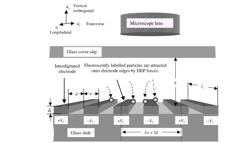
Figure 1.Diagram of a DEP collection experiment (using interdigitated electrodes fabricated on glass with widthw, interelectrode spacing

dand thicknessδe)notto scale. The movement of the fluorescently labelled particles, suspended in an aqueous medium, is monitored with a microscope.

(This figure is in colour only in the electronic version)

motion). The time-dependent accumulation of particles near the electrodes is called the DEP collection. Conversely, particle movement away from the electrodes diffusing into solution after the DEP driving force has been switched off is called particlerelaxation.

The application of DEP using planar electrodes means that the DEP forces are essentially short-ranged and ideal dielectrophoretic particle movement can be usefully described in several stages. Figure 2(a) depicts stages of an ideal DEP particle collection on a planar interdigitated electrode array:

(i) before DEP is switched on att =t0, where particles are

uniformly distributed,

(ii) t>t0particles driven by DEP forces collect on electrodes,

giving rise to a depletion zone above the array,

(iii) DEP forces continue to attract particles near the electrode surfaces, while above the depletion zone particles diffuse in so that the zone progressively moves away from the electrode surface, and

(iv) steady state, where DEP particle forces are balanced by diffusion (t→ ∞).

Two important parameters describing DEP collections (and relaxations) are, firstly, the initial time rate of increase in particles located near the electrodes or collection rate (immediately after the DEP force is switched on att = t0).

This is illustrated by the dotted line in figure 2(b). Secondly, the change in particle collection between DEP being switched on and the steady state—called the initial to steady-state transition, which is also illustrated in figure 2(b) byF(where Fis the normalized fluorescence intensity, see equation (11)). The first experiments on the use of DEP collections for determining dielectric properties of particles were summarized by Pohl (1978). Subsequent measurements of time-dependent

collections using optical absorption were reported by Talary and Pethig (1994) and Gascoyne et al(1994) who used the technique to measure the collections of cells and bacteria. Recently Milner et al (1998) and Suehiro et al (1999) also measured DEP collections using impedance methods. The latter developed a model which related the change in impedance to the cell concentration in an aqueous solution. However, very little work has been done in measuring and quantifying the time-dependent dielectrophoretic collection of sub-micron-scale particles on microelectrodes.

Asbury and co-workers (Asbury and van den Engh 1998, Asbury 1999, Asbury et al 2002) described measurements of the time-dependent DEP collection of DNA onto planar arrays and fitted these results by a single or double exponential profile. Their method quantitatively measured the peak values of the fluorescence near the electrode edges. These quantitative results of DNA trapping were performed at low AC frequencies ranging from∼10 Hz to 10 kHz (typically 30 Hz) and exhibited a dependence on electrolyte conductivity and on molecular weight. Fluorescence profiles of DNA being released and diffusing away from the electrode surfaces were also described. In this paper we describe analytical methods for quantitatively determining DEP time-dependent collections based on fluorescence microscopy and describe the application of this method to quantifying the high frequency time-dependent collection of 216 nm diameter carboxyl-modified latex microspheres. Video images of the fluorescently labelled beads collecting onto 10 µm width 10 µm gap planar interdigitated arrays under the action of DEP were processed using MATLAB 5.0TM _{software routines based on these}

(a)

(b)

Figure 2.(a) Diagram illustrating the one-dimensional (1D) movement of particles between a glass cover slip (upper boundary) and planar interdigitated electrode array (lower boundary). (i) shows the distribution of particles before the onset of DEP att=t0, (ii) shows particle collection near the electrodes immediately after applying the DEP force (t>t0) giving rise to the initial collection rate and a particle depletion zone above the array, (iii) shows continued particle collection at the electrodes (tt0) and the particle depletion zone moving upwards from the electrode plane, and (iv) shows the particle distribution at steady state (t→ ∞) where DEP particle forces are balanced by diffusion. (b) Graph of particle collection on the electrode array versus time corresponding to (a). The observed quantity is fluorescence

F(t)or particle numbern(t). The dielectrophoretic collection profiles for the arrangement can be described by the initial collection rate ˙

F(0)(or ˙n(0)) and the initial to pseudo steady-state change,F(orn). The initial collection rate ˙n(0)parameter (shown by the dotted line) pertains to times,t>t0, very soon after the DEP force is switched on when particles collect near electrodes solely under the action of the DEP force. Much later, attt0, the particle movement is governed by DEP and diffusion. At pseudo steady-state the movement by DEP is balanced by diffusion.

time-dependent fluorescent intensity profiles characterizing the particle collection around a representative electrode edge. The technique of spatially integrating particle fluorescence intensity around the electrode edges enables comparison of the particle collections with those predicted by theoretical simulations and can also be applied to fluorescently labelled DNA, viruses and proteins.

This paper also describes DEP collections for AC frequencies ranging from 0.5 to 5 MHz and extends the previous work of Bakewell and Morgan (2001) by including the electrical potential dependence of DEP collections for applied peak voltages V0=1–4 V. The experimental results

show that the dielectrophoretic response decreases as the frequency is increased and the voltage is reduced. These

experimental observations are expected from the reduction in the effective polarizability predicted by the Clausius– Mossotti function and the square-law voltage dependence of the DEP force. Comparisons with trends predicted from computer simulations using a Fokker–Planck equation (FPE) model (Gardiner 1985) indicates that other effects, such as electrohydrodynamic fluid motion or changes to the field gradient due to particles collecting on the electrodes, contribute to the quantitative differences between

theory and experiment. One consequence of these

Quantifying dielectrophoretic collections of sub-micron particles on microelectrodes 2. Theory

The FPE describes the behaviour, in space and time, of the concentration of particles in solution when subjected to an arbitrary external force. Under the influence of a time-averaged DEP force FDEP for non-interacting particles, the

concentrationcis related to the particle fluxJby

∂c

∂t = −∇·J= −

1

ζ∇·

   cαp

4∇|E|

2

FDEP   

+D∇ · ∇c (1)

where αp is the real part of the effective polarizability of

the particle (or dipole moment per unit electric field),∇ is the gradient operator, E is the electric field (peak value), ζ is the particle friction coefficient and D is the Boltzmann temperature-dependent diffusion constant, D = kBT/ζ. It

is understood x ≡ x,y,z,c ≡ c(x,t),J ≡ J(x,t). For a spherical particle,αp =4πr3εmRe{fCM}, where Re{fCM}is

the real part of the Clausius–Mossotti function,ris the particle radius and εm is the medium permittivity (Pohl 1978, Jones

1995, Morgan and Green 2003). Furthermore, the applied electrode voltage V0 and electric fieldE ≡ E(x)are related

throughE=V0K, whereKdefines the relationship between

the field and electrode geometry. The FPE can be solved numerically to give the particle concentration profile, provided that all the constants are known.

The DEP force on a particle is shown in equation (1) to depend on the effective polarizability αp and the square of

the electric field gradient, which can be calculated from the analytical solution to Laplace’s equation for the interdigitated electrodes (Morganet al2001). The FPE can be simplified to a two-dimensional (2D) problem for the interdigitated electrode array shown in figure 1, where the electrodes are considered to be infinitely long and therefore end effects can be ignored.

The time-dependent accumulation of particles, or collection profile, for the FPE reduced to 2D is given by the particle number n(t) per unit longitudinal length, which is related to the concentration over a cross sectional area A:

n(t)=

A

c(x,t)dx=

x2

x1 y2

y1

c(x,y,t)dxdy. (2)

An expression for theinitial collection rate of particles ˙

n(0)(·denotes time derivative) arriving at the electrodes can be determined by assuming the initial particle concentration to be uniform throughout the volume, implying, att =0,∇c=0=

∇2_{c. The initial collection rate is approximately proportional}

to the DEP force and can be used as a measure of the dielectric properties of the particles. Combining equations (1) and (2), it can be shown ˙n(0) ∝ αpV02n(0)/ζ, whereV0 is the applied

electrode voltage (peak) and n(0) is the initial number of particles. Thus, two collection experiments (labelled ‘1’ and ‘2’) using the same electrode array,ζ,n(0), etc, but assuming separateparameter values forV0andαp, will have theoretically

predicted collection ratios

˙ n2(0)

˙ n1(0)

= αp2V 2 02

αp1V

2 01

. (3)

The steady-state distribution of the particles occurs as t → ∞ and is governed by the balance of fluxes (DEP and diffusion). This is found by solving equation (1) with

∂c/∂t = 0. The ratios of steady-state particle concentration

for two collection experiments with separate parameter values forV0andαpare

c2(x,y,∞) c1(x,y,∞)

=Cexp

1 4kBT

(αp2V

2 02−αp1V

2

01)|K(x,y)| 2

(4) whereC is an arbitrary integration constant.

3. Experimental materials and methods

To perform a typical DEP particle collection experiment, 40µl of a fluorescently labelled 216 nm diameter bead suspension was micro-pipetted into the electrode array well. A 18× 18 mm2_{cover slip was placed over the suspension to reduce}

evaporation and to enable the array to be viewed under a microscope, as shown schematically in figure 1. The DEP experiment was recorded using a CCD camera (not shown) set with automatic gain control turned off. The video images were of the planar electrode array, of area∼=190µm×250µm.

3.1. Planar interdigitated electrode arrays

The planar interdigitated electrodes, shown in figure 1, were fabricated on glass microscope slides using standard positive S1818 resist photolithography and metallic vapour deposition techniques (Pacansky and Lyerla 1979). The Ti–Pd–Au electrodes had thicknessδe =120 nm, width=w=10µm,

gap = d = 10 µm and length lz ∼= 2 mm. Eight

separately addressable electrode arrays were fabricated on a slide spanning a total rectangular planar area of 200 mm2_{. Two}

narrow cover slips, fixed along the long sides of the rectangular 8-electrode array, enabled the heighthof the 18×18 mm2_cover

slip above the electrode plane to be well controlled. Using a 40µl microsphere droplet resulted inh∼=200µm.

The electrode arrays fabricated on glass were in turn mounted on a printed circuit board. As indicated in figure 1, neighbouring electrodes in the array were supplied with electrical potentials of opposite (±V0) polarity. The

frequency and voltage supplied to the electrodes was controlled by a digital data synthesizer (DDS) and the electrode potentials were switched on/off manually and monitored by an oscilloscope.

3.2. Preparations of latex microspheres and experimental measurements

The model colloidal particles used for DEP experiments were 216 nm diameter carboxyl-modified polystyrene fluorescent microspheres FluoSpheres®_{(Molecular Probes, Eugene, USA,}

microsphere suspension wasσm=1.7 mS m−1(Jenway 4701,

RS Components, UK). Assuming the density of polystyrene is 1.05 g cm−3 _{the final microsphere concentration used at}

the start of the DEP experiments was estimated as cV = 3.613×1015m−3orcV ∼=4×10−3µm−3(Bangs 1997). This value approximately agreed with the number of beads visible over the planar array before the onset of DEP, assuming a 1µm vertical depth-of-focus.

3.3. Development of video image processing software

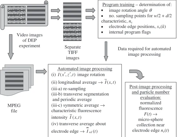
Figure 3 shows typical recorded video images of a DEP experiment before and after applying the electric field. Both images are approximately half-length frame size (540×360 pixels) and have been cropped and juxtaposed for illustrative purposes. Figure 3(a) shows the planar interdigitated array before application of the electric potential where particles exhibit Brownian motion in the suspending medium. This corresponds to figure 2(a)(i). Figure 3(b) shows particle collection in the immediate vicinity of the electrodes under the action of positive DEP about five seconds after applying the field. The particle concentration in the plane immediately above the electrodes is depleted—as depicted in figure 2(a)(ii). The time-dependent particle concentration on the electrodes is determined by experimental conditions, in particular the polarizability which is a function of frequency. Consequently, an accurate measurement of bead concentration as a function of time should enable a quantification of the frequency-dependent DEP force.

In order to achieve quantitative evaluation we have developed the following image processing technique outlined schematically in figure 4. Video footage is captured using a miroVIDEO®DC 30 (CA, USA) frame grabber and converted by Photo-Paint 6.0® (Corel, CA, USA) from an AVI file to either a sequence of TIFF images or a MPEG movie file (Haskell et al 1997), as indicated in figure 4. The capture rate ranges from 1 to 25 frames s−1_{. A}

time-dependent fluorescence profile of the collection experiment is constructed by sequentially image processing each frame automatically using a user-interactive program written in MATLAB 5.0TM _{(programs available from the author). The}

image processing takes advantage of the transverse periodicity and symmetry of the array. Figure 4 outlines the conversion of the time sequence of video image intensities recorded from the camera, written asI(x,z,t), to the fluorescence intensity F(t)representing DEP particle collection near a representative electrode edge. A key intermediate step is the transformation of the 2D intensity of each frame to a 1D intensity plot with transverse dimensions periodically and symmetrically averaged to an electrode half-width and half-gap (w/2 +d/2). This intensity, representing the fluorescence of the array, is called a characteristicintensity, I˜(x,t) (written in discrete form asI(i,˜ t)) and can be evaluated as a function of time and experimental conditions, such as frequency and voltage.

A simpler method of quantifying particle collection using fluorescence microscopy was demonstrated by Asbury and van den Engh (1998) and Asbury (1999). These authors quantified DNA collection by averaging the height of the fluorescence signal from each electrode strip. We have extended this procedure and integrated the signal in a well-defined region

either side of the electrode edge (i.e. in the transverse direction). Relating time-dependent particle collection to the area of the fluorescent signal has the advantage of being able to directly quantify the number of particles in a defined region on the electrodes and facilitates a more accurate comparison with simulation.

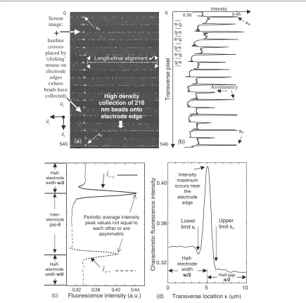
3.3.1. Image processing set-up—array geometry. Each frame is processed automatically to generate a time-dependent particle collection profile. In order to set up the automated frame processing, data are entered into the software about the geometry of the array using a sample of TIFF images for ‘training’ the program, as outlined in figure 4. To ensure correct alignment for pixel averaging the image was often rotated, typically through an angle−0.3◦ θ 0.3◦, since an angular error of 0.1◦over 720 pixels horizontally resulted in a mismatch of approximately 1 pixel in the ‘vertical’ axis of the screen image. Figure 5(a) shows a rotated video frame of a DEP collection, cropped for illustration, where the angular alignment of the electrode edges concurs with the horizontal axis of the screen.

To construct the characteristic intensity I(r,˜ t) for an electrode half-width and half-gap (w/2 +d/2), each electrode and neighbouring gap is paired and the number of electrode-gap pairs, npr, is selected in the program. The number of

edges is ned = 2npr + 2. In figure 5(a) the transverse

position of the first and last electrode edges is denoted as xa andxb. The number of pairs and edges in this figure is npr = 8 and ned = 18. The location of electrode edges in

the transverse direction is entered by visual inspection using the mouse-controlled hairline. Each registered location is shown by the cross, ‘+’, marker superimposed on the image in figure 5(a) and is written as x+(k), where k ∈ [1,ned].

The number of pixels between electrode edges varies by as much ±5% whereas the electrode dimensions are known to remain constant, w = d = 10 µm. To circumvent this problem, the longitudinally averaged intensity is re-sampled such that each electrode width and gap between xa and xb receives the same number of samples. The number of sample points forw/2=d/2 is given byn1/2. Hence the number of

sample points for eachw/2 +d/2characteristicis therefore nc=2n1/2. Typically, 30n1/250. Parameter values for θ,nc,x+(k)and internal program flags are stored for use in

automated processing, as indicated in figure 4.

Quantifying dielectrophoretic collections of sub-micron particles on microelectrodes

Figure 3.Positive DEP collection of 216 nm diameter fluorescent microspheres ontod=w=10µm interdigitated electrodes (a)∼1 s before the DEP force was applied (b)∼5 s after the DEP force was applied.

MPEG file

Video images of DEP

experiment _Separate TIFF images

Program training – determination of: image rotation angleθ no. sampling points forw/2 +d/2 characteristic,nc

electrode edge positions,x+(k) internal program flags

Automated image processing (i)I(x′,z′,t)image rotation (ii) longitudinal average→ I(x,t) (iii-a) re-sampling

(iii-b) transverse segmentation and periodic average (iii-c) symmetric average→ characteristic fluorescence intensity~I(x,t)

(iv) transverse average about electrode edge→ Ied(t)

Data required for automated image processing

Post-image processing and particle number

evaluation: normalized fluorescence F(t)→ micro-sphere collection near electrode edgene(t)

Figure 4.Schematic of image processing software that converts the 2D fluorescence intensityI(x,z,t)recorded in each video frame to normalized fluorescenceF(t)representing DEP particle collections (and relaxations) in the near vicinity of a electrode edge representative of the interdigitated electrode array.

(i) Each frame is either a TIFF image, or decoded MPEG image, and is rotated by θ such that I(x,z,t) → I(x,z,t), whereθ is specified by the training program described in the previous section. The rotated image, I(x,z,t), is written in discrete formI(r,c,t)suitable for pixel averaging, whererandcare respectively pixel values for each rowrand columnc.

(ii) The longitudinal fluorescence intensity average along the columnscfor each pixel location (rowr) in the transverse direction is given by

¯

I(r,t)∼=z cmax

c=1

I(r,c,t)

z cmax

c=1

1

= 1

cmax cmax

c=1

I(r,c,t) (5)

wherez is the finite differential increment along the longitudinal direction, uz, and cmax = 720 is the total

number of column pixels. A plot of the average intensity

¯

I(r,ti) extracted from the program for the example greyscale frame of figure 5(a) is shown in 5(b). The plot shows the presence of beads at the edges corresponds to peaks in the average intensity and the values are generally higher over the gold electrodes than the gaps since the former reflect more scattered light.

(iii) (a) Re-sampling of the longitudinally averaged intensity

¯

I(r,t)is performed by the following mapping:

¯

I(r,t) Intensity

→ ¯ I(x,t) Interpolate

→ ¯ I(xs,t) Resample

→ ¯ I(j,t) Reconstructed Intensity

. (6a)

0

(a)

Screen image:

+

hairline crosses placed by ‘clicking’ mouse on electrode edges (where beads have

collected)

540

z u

x u y u

Longitudinal alignment

High density collection of 216

nm beads onto electrode edge

xb xa

(b)

0.30 0.45

Intensity 0

540

Tr

ansverse

p

ix

el

xa

xb

Asymmetry

Transverse locationx(µm)

Half-gap d/2

Char

acteristic

fl

u

oresc

ence

intensit

y

Half-electrode

width

w/2

Intensity maximum occurs near

the electrode

edge

0.36

0.32 0.40

0 5 10

(d)

0.32 0.36 0.40 0.44

Fluorescence intensity (a.u.)

Inter-electrode gapd

Half-electrode widthw/2

Half-electrode widthw/2

g e I₋ ~

e g I ₋ ~

Periodic average intensity peak values not equal to

each other or are asymmetric

(c)

e-g

g-e e-g

g-e

Lower limitxl

Upper limitxu e-g

g-e

Figure 5.(a) Positive DEP collection image processed frame (37 s after DEP force applied) with (b) associated average longitudinal greyscale intensity for each transverse pixel. (c) is the periodic average of the fluorescence intensity forI˜e−g(x,t)(——) andI˜g−e(x,t) (— — —) for the two segment types shown in (b). The symmetric average ofI˜e−gandI˜g−eis thew/2 +d/2characteristicintensityI˜(x,t), (d), that represents the pixel intensity for the entire video frame.

{1,2, . . . ,ned − 1} and i = {1,2, . . . ,nc} assigns

transverse locations where the interpolated intensity

¯

I(x,t)is re-sampled at locations

xs(j)=x+(k)+i[x+(k+ 1)−x+(k)]/nc. (6b)

(b) To construct thew/2 +d/2 characteristic intensity, the fluorescence profile in the transverse direction between xa and xb is segmented into two transverse types and averaged. Several examples are illustrated in figure 5(b), the segments labelled ‘e–g’ signify pixels located within the transition from electrode half-width to half-gap (moving down figure 5(b) fromxatoxb), and the segments labelled ‘g–e’ signify pixels lying within the transition from half-gap to electrode half-width. The intensities along each of the two segment types are averaged over

the electrode and gap pairsnpraccording to

˜

I(i,t)

˜ Ie−g

= 1

npr npr

k=1

¯

I(i+n1/2+ 2nc(k−1),t)

Ie−g segments

∀i = {1,2, . . . ,nc} (7a)

˜

I(i+nc,t)

˜ Ig−e

= 1

npr npr

k=1

¯

I(i +n1/2+ 2nc(k−1)+nc,t)

Ig−e segments

∀i = {1,2, . . . ,nc} (7b)

where thetildasymbol (∼) denotes a ‘periodic’average profile spanning the intervalw/2 +d+w/2 (one electrode width and gap) and subscripts ‘e–g’ and ‘g–e’ correspond to the examples in figure 5(b). Then1/2 end segments

Quantifying dielectrophoretic collections of sub-micron particles on microelectrodes

The variation of the peak intensities in figure 5(b) is approximately proportional to the number of beads accumulated at each of the electrode edges. Some of the intensities at the edges showed a marked asymmetry, as depicted in figure 5(b), and are clearly shown in the periodic average, figure 5(c). This is not expected from the theory that predicts the DEP force and hence particle collection (for positive DEP) on both sides of any electrode edge should be the same. Fluctuations similar to these have been reported by other workers (Asbury and van den Engh 1998).

(c) The symmetric average is obtained by rotating theI˜g−e

profile by 180◦, as shown in figure 5(c), and superimposing onto theI˜e−gprofile. The average yields thecharacteristic

intensityI˜(x,t), written indiscreteform asI˜(i,t):

˜

I(i,t)= 1₂

˜

I(i,t) Ie−g

+I(˜2nc+ 1−i,t)

Ig−erotated 180◦

∀i= {1,2, . . . ,nc}. (8)

TheI˜(i,t)for the example in figures 5(a)–(c) is shown in figure 5(d) (redrawn with the transverse axis horizontal).

˜

I(i,t) is called the characteristic intensity since it represents the average intensity alonguzand the periodic and symmetric average across ux. The periodic and symmetric properties of the array enables the transverse regionux to be divided into ‘cells’. Thus I˜(i,t)spans 0x xc, wherexc= w+₂d. Figure 5(d) shows the peak

of the intensity due to bead accumulation is located close to the electrode edge, positioned atxe = w₂. The

time-dependentw/2+d/2 fluorescence intensity characteristic,

˜

I(i,t), is stored as a matrix where each row represents a time ‘slice’ att=tj, the first column is the time (s) and the remaining columns are the associated intensity profiles. An example of a 3D plot of the matrix resulting from particle collection for thew/2 +d/2 transverse interval is shown in figure 6.

(iv) The time-dependent intensity profile for particle accu-mulation is determined from the characteristic intensity

˜

I(x,t) by averaging in the transverse direction ux typ-ically for a small region of interest centred about the electrode edge, xe. This interval is specified by xu–xl,

where xl and xu are the lower and upper limits

illus-trated in figure 5(d) and are related to the integer values il and iu: xl = (il−1)x = (il−1)(w+₂d)/(nc −1), xu=(iu−1)x=(iu−1)(w₂+d)/(nc−1), withx the

finite differential increment along the transverse direction,

ux.

The average ofI˜(x,t)overxu–xlis evaluated using the

trapezium rule:

I =

ed(t)= xu

xl

˜

I(x,t)dx

xu

xl

dx ∼= Iˆed(t) iu−il

= 1

iu−il _˜

I(il,t)+I˜(iu,t)

2 +

iu−1

i=il+1

˜

I(i,t)

(9)

where the subscript ‘ed’ denotes the average is over the transverse interval ‘in the near vicinity of the electrode edge’ and the double overbar denotes spatial averages in both directions ux and uz. If the limits are reasonably close to

the electrode edge xe = w₂, but not too close, the integral

is a measure of the fluorescence intensity of particles located ‘about the electrode edge’. Ifxl is too low andxu too high,

the change in intensity ‘about the electrode edge’ is poorly represented. On the other hand, if xl and xu are close to

each other at the edge, xe = w₂, the integral Ied(ti)is prone to changes in the precise shape of I(x˜ ,t). Small changes in the shape of I˜(x,t) can occur due to misjudgements of the position of the electrode edges during image processing set-up.

3.3.3. Post-image processing: normalized fluorescence intensity. Fluctuations in the fluorescent light source often occur with mercury lamps (Ploem and Tanke 1987) which results in small-time variations in Ied(t). These fluctuations

can be smoothed by normalizing Ied(t) with respect to the

average intensity I˜(i,t) representing the entire w/2 +d/2 transverse interval. This is thetotalintensity,=IT(i,t):

I =

T(t)=

ˆ

IT(t) nc−1

= 1

nc−1 _˜

I(1,t)+I˜(nc,t)

2 +

nc−1

i=2

˜

I(i,t)

.

(10) The normalized intensity can be found by dividing equations (9) by (10) and this approach is suitable, for example, for dielectrophoretic measurements of DNA collecting over the interelectrode gap (Bakewell 2002). For colloidal particles collecting near the electrode edges, the normalized fluorescence intensityF(t)is more suitably expressed in terms of=Ied(t)andI

=

lu(t), which is the average intensity for thex

intervalsawayfrom the edge, 0x xlandxux w₂+d:

F(t)= I =

ed(t)

I =

lu(t)

= Iˆed(t)/[iu−il]

[IˆT(t)− ˆIed(t)]/[il−1 +nc−iu]

(11)

where Iˆed(t)and IˆT(t) are given by equations (9) and (10).

The post-image processing step of fluorescence normalization is indicated in figure 4 and an example of F(t) evaluated using I˜(x,t), shown in figure 6, is illustrated in figure 7. In general, normalization tends to increase the sensitivity of the rise profile and in the hypothetical case, where particle collection onto the electrode edge causes almost entire particle depletion elsewhere such that=I ed(t) = 0 and I

=

lu(t) → 0,

then F(t) → ∞. In practice, DEP experiments do not exhibit extreme particle depletion, except when the aqueous suspending medium has almost entirely evaporated, so (11) is satisfactory to use.

3.3.4. Determining DEP collections from normalized fluorescence intensity. The fluorescence intensity,=Ied(t)can

be written in terms of the fluorescence from particles within a small≈1µm vertical depth-of-focus (located close to the electrode plane) and fluorescence from particles above the focal plane in the bulk solution. A similar phenomenological model for =Ilu(t) can also be written. Combining both

expressions using (11), the temporal change in normalized fluorescence for the DEP collection time intervalt–t0is

F(t)=F(t)−F(t0)=k[ne(t)−ne(t0)] +εf(t)

w/2

d/2 )

, ( ~

t x I

Frame number

x u

Half electrode

width, half-gap Time (s)

Time

~ steady state

P2 P1

P3

t= 0 s P4

Figure 6.Example of a characteristicw/2 +d/2 fluorescence intensityI˜(x,t)of a sequence of video frames that shows DEP particle collection and relaxation about a representative electrode edge for the experimental condition,V0=2 V, f =1 MHz.

0 20 40 60 80 100 120 140 160 180 200

0.95 1 1.05 1.1 1.15 1.2

Frame number

t= 0 (DEP starts) Timet(s) t= 137 s

FA(t) collection profile, or ‘rise’, fitted by a double exponential function

FA(t) relaxation profile, or ‘fall’, fitted by single

exponential

Norm

alized

Fluorescenc

e

F

(

t

)

FB(t)

FB(120) approaching steady state

FC(t)

FA(t)

FC(120) practically at steady state

FA(t):Vo= 2 V , f= 1 MHz

FB(t):Vo= 2 V , f = 0.5 MHz

FC(t):Vo= 2 V , f = 2 MHz

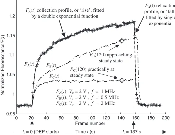
Figure 7.Examples of normalized fluorescenceF(t)for DEP collections and relaxations for different experimental conditions. TheFA(t) collection and relaxation profile was evaluated fromI˜(x,t), illustrated in figure 6.

where ne(t) is the number of particles at an electrode edge

of a representative cell for xl x xu, k is a constant

and the error is εf. The subscript ‘e’ denotes the particle number is determined byexperimentviaFand the particles are in the near vicinity of the electrode edge. The constant k includes optical parameters such as the numerical aperture of the objective, re-absorption of emitted light, quantum efficiency of the fluorophore, absorption, scattering and excitation absorbance. The constant also includes the effect of fluorescence in the transverse region away from the edge, 0 x xland xu x xc, which is assumed to remain

unchanged during the course of the experiment.

Essentially, the background fluorescence within the plane of focus is eliminated by assuming it remains unchanged for

t > t0. The error termεf accounts for any deviation from these together with other assumptions and is typically small,

εf(t) <0.1kne(t). This means the difference in normalized

fluorescence about the electrode edge is approximately proportional to the difference in particle concentration near the edge. Re-arranging (12), and without loss of generality settingt0=0, at timetthe change in particle number located

near the electrode is approximated by

ne(t)=[F(t)−εf(t)]/k∼=F(t)/k. (13)

Quantifying dielectrophoretic collections of sub-micron particles on microelectrodes

0.00 0.05 0.10 0.15 0.20

0 20 40 60 80 100

∆n =2.92988 + 860.05119∆F - 2109.55941∆F

2

from collection 2 from collection 1

∆

n=n

(

tj

)–

n(0)

∆F = F(tj) - F(0)

Individual beads in high density clusters along electrode edges cannot be

discriminated

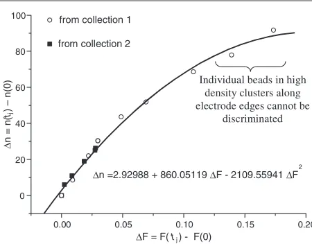
Figure 8.Relationship between the change in average bead number ne(collected on the electrode edges) and change in fluorescence F.

is mapped in figure 8 for two sets of data and was fitted to a second-order polynomial using Origin 4.1TM_{. The relationship}

between ne andFis linear for lowne. For highF,

however, individual beads lying on the electrode edges in groups or clusters are practically impossible to distinguish. Therefore, the value of the constant was taken from the linear term in the polynomial,k =1/860.

Considering infinitesimal time increments, t = t0+t

and taking limitst→0+, (13) leads to

˙

ne(0)=F(˙ 0)/k (14)

where the dot ‘·’ denotes the time derivative and is understood to be in the +tdirection att0=0. Experimental values for the

initial particle collection rate can be estimated by measuring the gradient of Fover small increments in time immediately before and after the DEP force is applied, ˙F(0) ∼₌ δF/δt. An alternative and more robust method deduces ˙F(0) from the entire collection characteristic,F(t). The characteristic is fitted to an analytical function, typically a double exponential, and the function is differentiated with respect to time. The equation for the DEP collection starting att =t0suitable for

fitting with commercially available software, such as Origin 4.1TM_{, has the form}

F(t)=F0−F1exp[−(t−t0)/τe1]−F2exp[−(t−t0)/τe2]

(15) whereτe1andτe2are the rise times and componentsF1>0 and F2>0. Differentiating with respect to time, settingt=t0=0

and using (14), the initial collection rate is given by

˙ ne(0)=

˙ F(0)

k =

F1/τe1+F2/τe2

k . (16)

4. Results and discussion

The DEP collections and relaxations for the 216 nm diameter fluorescently labelled microspheres were investigated for two independent variables: applied DEP frequency, f, and peak potential,V0. Three different frequencies were applied using V0=2 V: f =500 kHz, 1 MHz, and 2 MHz. No collections

were observed for f 3 MHz. Collections using three peak

voltages,V0 =1, 2 and 4 V, were conducted at f =2 MHz.

In each experiment the particlecollectionwas observed for 2–3 min, followed by particlerelaxation(DEP switched off, V0=0 V), which was observed for 30–60 s.

Since particle collections tended to vary over the area of an array, collections and relaxations were performed insets ofthreeexperiments. In each set, the same area of the array was used to record particle collections (and relaxations) for all of the three possible states of the independent variable (f orV0). This enabled the collections to be compared with

each other to avoid, as far as possible, any disparities in bead density arising from variations in electrode edge definition during micro-fabrication.

4.1. An example of DEP collection and relaxation

A typical characteristic intensityI˜(x,t)is illustrated in figure 6 for a 216 nm diameter fluorescent bead DEP collection on the planar interdigitated electrode array described in section 2 with experimental conditions V0 = 2 V and f = 1 MHz. The

characteristic was generated using expressions (5)–(8). The first feature ofI˜(x,t)is that 2 min after the onset of DEP, the collection over the electrode edge is substantially at a steady state. The video was frame grabbed at a rate of 1 frame s−1_{, so}

the entire collection and relaxation required about 200 frames to image process.

The second feature of figure 6 is that a small decrease in fluorescence occurs over the lower and upper transverse intervals after the onset of DEP (t = 0 s), at points located near P1 and P2. The precise cause of this reduction is not

entirely clear but it generally occurs with all DEP experiments, so it is not attributed to fluctuations in the source intensity. Restoration of the fluorescence also occurs after the DEP is switched off, as shown near points P3 and P4. The

fluorescence reduction (and restoration) phenomena tend to be more pronounced when the DEP force is strong, so it is likely to be due to DEP-induced depletion of particles within and above the focal plane. Fluorescence depletion and restoration affects no more than about 10% of the intensityI(x,˜ t)so the approximation for the errorεf(t)in (13) applies. As shown in figures 5(a)–(d) the intensity is slightly higher over the (gold) electrode than the (glass) gap since the former reflects more light. Small temporal variations in the source are evident and can be minimized or cancelled by normalization.

Spatially averaging and normalizing I˜(x,t) using equations (9)–(11) led to a collection and relaxation normalized fluorescence profile,FA(t), shown in figure 7. The

data points (denoted ‘+’) constituting the collection, or ‘rise’, were fitted with Origin 4.1TM _{for 120 s, yieldingτ}

e1 ∼= 3

and τe2 ∼= 45 s. Data for the relaxation, or ‘fall’, were

fitted to a single exponential τe3 ∼= 2 s. The double and

single exponential fits have been superposed on the data points as shown (— — —). Many collections resembled the ‘well rounded’ form ofFA(t), where it was clear the collection was

substantially at steady state (zero time rate of fluorescence change) at 120 s and exhibited short rise times. An example of this isFC(t)with parametersV0=2 V and f =2 MHz, where τe1 ∼=2 andτe2 ∼=9 s. Other collections, however, deviated

τe1∼=5 andτe2∼=170 s. The relaxation fall times forFB(t)

and FC(t)wereτe3=∼1 s andτe3∼=2 s, respectively2.

Figure 7 highlights a number of key characteristics typical of DEP collections and relaxations and these are discussed further in the next section. The most important observation is that the magnitude of the fluorescence profile, or increase in fluorescence after the DEP force is switched on,F(t), and the initial rate of change of fluorescence, ˙F(0), are key measures of the DEP strength. ProfilesFA(t),FB(t)andFC(t)in figure 7

show a respective decreasing DEP strength and it is clear

FA(t) > FB(t) > FC(t)and ˙FA(0) > F˙B(0) >F˙C(0),

that is, both F(t) and ˙F(0) concurrently follow the same trends.

4.2. Quantitative measurements

Profiles for the time-dependent normalized fluorescenceF(t) were evaluated as described for the above example. The number of sample points for each (w/2 +d/2) characteristic wasnc=100 and the number of electrode pairs wasnpr=8.

The image processing parameters all had the propertyiu−il=

16, i.e. the transverse length ofthex–ycross section designated collection area, using the expressions for the lower and upper limits in (9) withw = d = 10µm, wasx = xu−xl ∼=

1.6µm. Typically, the integer values ranged fromil=43 to

49 andiu =59 to 65, depending on the transverse alignment

of the frames used for the set-up described in section 3.3.1. The differences in the normalized fluorescenceF(120) = F(120)− F(0)were calculated using (12). All collections, except for theV0= 1, f =2 MHz case, were best fitted by

a double exponential (15) using Origin 4.1TM_{. The relaxation}

after collection was best fitted by a single exponential, with fall amplitude and time,F3andτe3. Values for the initial collection

rates ˙F(0) were computed using (15) with fitted amplitudes F1 and F2 and timesτe1and τe2and values were confirmed

using a linear fit to the fluorescence gradient, δF/δt. The particle parameters ˙ne(0)/ne(0) and ne(120)/ne(0) were

evaluated using equations (13) and (16) using a nominal value ofne(0) = 2.8. This enabled a comparison with theoretical

predictions using an FPE model.

The values of the collection parameters, including rise and fall timesτe1,τe2andτe3, are shown in table 1 (rise amplitudes

F1andF2and fall amplitudeF3are omitted for clarity).

Table 1 shows that the values of the fluorescence change at t = 120 s, F(120) = F(120) − F(0) and ˙F(0) concurrently follow the same trends as illustrated in figure 7 and both parameters, ne(120)/ne(0) and ˙ne(0)/ne(0), are

key measures of the DEP response. The values of the particle parameters ne(120)/ne(0)and ˙ne(0)/ne(0)for set

I with a constant peak voltage V0 = 2 V and variable

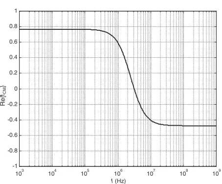
frequency f = 0.5, 1, 2 MHz show the DEP response decreases with increasing frequency. This is expected since equation (1) shows the DEP force is proportional to the effective polarizability of these microspheres predicted by the real part of the Clausius–Mossotti function, Re{fCM},

plotted in figure 9. Figure 9 shows the Re{fCM}for the same

low conductivity medium as used in the DEP experiments decreases 3×from 0.5 to 2 MHz and is negligible at 3 MHz— consistent with the observation of no DEP collections for

2 _{The curve fitted for the relaxationF}

C(t)has been removed for clarity.

103 104 105 106 107 108 109 -1

-0.8 -0.6 -0.4 -0.2 0 0.2 0.4 0.6 0.8 1

f(Hz)

Re{

fCM

}

Figure 9.Frequency-dependent real part of the Clausius–Mossotti function Re{fCM)used for predicting the polarizability of 216 nm diameter latex microspheres in a low conductivity medium (1.7 mS m−1_).

f 3 MHz. The values of the collection parameters

ne(120)/ne(0) and ˙ne(0)/ne(0) in table 1 for set II with

constant frequency f = 2 MHz show the DEP response

markedly decreases with voltage, as predicted from the theory that predicts the DEP force∝V2

0. The rise timesτe1andτe2

are consistently higher than the fall timeτe3 for substantial

DEP collections and this is expected of a system where the collection occurs under a combination of deterministic and stochastic forces, in contrast to relaxation that occurs solely by diffusion.

Each of the values in table 1 is an average of three experimental values compiled from the six sets (of three experiments) and there was statistical variation in the F(t) profile between each experiment under the same V0 and f

conditions. Figure 7 indicates this statistical variation for the condition V0 = 2 V by illustrating that the DEP collection

profile FA(t) at f = 1 MHz is greater than for FB(t) at f = 0.5 MHz for this particular DEP experiment—-which is in contrast to the average shown in table 1. The reason for these variations between substantially strong DEP collections is not entirely clear at this stage but may be due to fluid motion (Ramos et al 1998, 1999, Green et al 2000a, 2000b) that confounds the observations and needs further investigation.

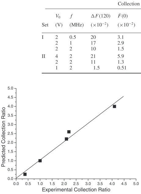
A brief comparison of the collection parameters with theoretical predictions is illustrated in figure 10. The initial collection rate ( ˙ne(0)/ne(0)) was normalized with respect to

the value at f = 1 MHz andV0 = 2 V (an average of the

two, approximately equal, values listed in each set was taken). The predicted parameter was obtained from equation (3) using the Clausius–Mossotti function which is plotted in figure 9. Figure 10 shows this parameter for different frequencies and voltages, using the data presented in table 1. Also shown is a linear regression to the data, which has a slope of unity and indicates that measurement of the ratios of the initial collection rate is an excellent indicator of the dielectrophoretic properties of the system. In contrast, the ratios of the initial to steady-state transition (ne(120)/ne(0)) are inconsistent with theoretical

Quantifying dielectrophoretic collections of sub-micron particles on microelectrodes

Table 1. Experimental frequency and voltage-dependent DEP particle collection and relaxation data. The values are an average of three separate experiments which have been rounded to two significant figures.

Collection

Relaxation

V0 f F(120) F˙(0) τe1 τe2 τe3 Set (V) (MHz) (×10−2_{) (×10}−2₎ ne(120)

ne(0) ˙

ne(0)

ne(0)

(s) (s) (s)

I 2 0.5 20 3.1 58 9.4 4.1 220 1.2

2 1 17 2.9 48 8.9 2.9 35 1.6

2 2 10 1.5 29 4.6 2.9 17 1.4

II 4 2 21 5.9 62 18 2.3 17 1.4

2 2 11 1.3 32 4.1 5.8 88 1.5

1 2 1.5 0.51 4.2 1.6 3.5 — 2.5

0.0 0.5 1.0 1.5 2.0 2.5 3.0 3.5 4.0 4.5 5.0

0.0 0.5 1.0 1.5 2.0 2.5 3.0 3.5 4.0 4.5 5.0

Pr

edicted

C

o

llect

ion

R

a

tio

Experimental Collection Ratio

Figure 10.Correlation between experimental and predicted values of the initial collection rate. The ratios of the parameter were normalized with respect to their values at f =2 MHz andV0=2 V.

entirely clear and may be related to limitations in the model or to experimental effects such as mentioned above.

5. Conclusion

Video recorded fluorescence microscopy was used to measure and quantify the time-dependent dielectrophoretic collections of 216 nm diameter carboxyl-modified latex microspheres onto 10µm width 10µm gap planar interdigitated electrodes as a function of frequency and applied voltage. Analytical methods utilizing the geometrical properties of the electrode array and implemented in MATLAB 5.0TM _{were used to characterize}

the dielectrophoretic response of the microspheres. The time-dependent particle collections, in the near vicinity of each electrode edge, were characterized by three parameters: the initial DEP collection rate, the transition from initial to pseudo-steady-state at 120 s and the rise time. The relaxation profiles were summarized by the fall time parameter.

Collection time profiles exhibited a clear decrease in the DEP response as the frequency increased from 500 kHz to 2 MHz and this trend concurred with the reduction in the real part of the effective polarizability of the microspheres predicted by the Clausius–Mossotti function. The DEP response also decreased as the peak electrical potential was reduced from 4 to 1 V and the trend concurred with a square-law voltage dependence of the DEP force. The trends in the

rise times are not as conclusive. However, the results show rise times are greater than the fall times for appreciable DEP collections, as expected from system dynamics. The initial DEP collection rate parameter was in good agreement with the predicted variation in DEP force at different applied voltages and frequencies, as given by equation (3). However, the initial to pseudo-steady-state transition was not as sensitive as theory predicts. Both parameters are dependent on particle concentration but in practice this technique is only suitable for a limited range of concentrations. At low concentrations there are insufficient particles collecting during a reasonable time frame to yield useful data; at high concentrations particle interactions and background fluorescence complicate the analysis. The analytical methods described in this paper show a promising application for characterizing the dielectrophoretic collections of sub-micron particles using fluorescence microscopy.

References

Abramowitz S 1996 Towards inexpensive DNA diagnosticsTrends Biotechnol.14397–401

Asbury C L 1999 Manipulation of DNA using nonuniform oscillating electric fieldsPhD DissertationUniversity of Washington, Seattle, USA

Asbury C L and van den Engh G 1998 Trapping of DNA in nonuniform oscillating electric fieldsBiophys. J.741024–30 Asbury C L, Diercks A H and van den Engh G 2002 Trapping of

DNA by dielectrophoresisElectrophoresis232658–66 Bakewell D J 2002 Dielectrophoresis of colloids and

polyelectrolytesPhD DissertationUniversity of Glasgow, Scotland, UK

Bakewell D J and Morgan H 2001 Measuring the frequency dependent polarisability of colloidal particles from

dielectrophoretic collection dataIEEE Trans. Dielectr. Electr. Insul.8566–71

Bangs 1997Technical Notes #49 and #206Bangs Laboratories Inc., USA

Cheng J, Sheldon E L, Wu L, Uribe A, Gerrue L O, Carrino J, Heller M J and O’Connell J P 1998 Preparation and hybridisation analysis of DNA/RNA fromE.Colion microfabricated bioelectronic chipsNature Biotech.16541–6 Chou C-F, Tegenfeldt J O, Bakajin O, Chan S S, Cox E C,

Darnton N, Duke T and Austin R H 2002 Electrodeless dielectrophoresis of single- and double-stranded DNA

Biophys. J.832170–9

Crippen S M, Holl M R and Meldrum D R 2000 Examination of dielectrophoretic behaviour of DNA as a function of frequency from 30 Hz to 1 MHz using a flexible microfluidic test apparatusProc. Micro Total Analysis Systems

Cui L, Holmes D and Morgan H 2001 The dielectrophoretic levitation and separation of latex beads in microchips

Electrophoresis223893–901

Gardiner C W 1985Handbook of Stochastic Methods for Physics, Chemistry, and the Natural Sciences(Berlin: Springer) Gascoyne P R C, Noshari J, Becker F F and Pethig R 1994 Use of

dielectrophoretic collection spectra for characterizing differences between normal and cancerous cellsIEEE Trans. Ind. Appl.30829–33

Green N G, Ramos A, Gonzalez A, Morgan H and

Castellanos A 2000a Fluid flow induced by non-uniform AC electric fields in electrolytic solutions on micro-electrodes. Part I: experimental measurementsPhys. Rev.E614011–8 Green N G, Ramos A and Morgan H 2000b AC electrokinetics: a

survey of sub-micrometre particle dynamicsJ. Phys. D: Appl. Phys.33632–41

Haskell B G, Puri A and Netravali A N 1997Digital Video: An Introduction to MPEG-2(Boston: Kluwer)

Jones T B 1995Electromechanics of Particles(Cambridge: Cambridge University Press)

Milner K R, Brown A P, Betts W B, Goodall D M and Allsopp D W E 1998 Analysis of biological particles using dielectrophoresis and impedance measurementBiomed. Sci. Instrum.34157–62

Morgan H and Green N 2003AC Electrokinetics: Colloids and Nanoparticles(Baldock, Herts: Research Studies Press) Morgan H, Izquierdoa G, Bakewell D, Green N G and

Ramos A 2001 The dielectrophoretic and travelling wave forces for interdigitated electrode arrays: analytical solution using Fourier seriesJ. Phys. D: Appl. Phys.341553–561 Pacansky J and Lyerla J R 1979 Photochemical decomposition

mechanisms for AZ-type photoresistsIBM Res. Dev.2342–55 Ploem J S and Tanke H J 1987Introduction to Fluorescence

Microscopy(Oxford: Oxford University Press) Pohl H A 1978Dielectrophoresis(Cambridge: Cambridge

University Press)

Ramos A, Morgan H, Green N G and Castellanos A 1998 AC electrokinetics: a review of forces in microelectrode structures

J. Phys. D: Appl. Phys.312338–53

Ramos A, Morgan H, Green N G and Castellanos A 1999 AC electric-field-induced fluid flow in microelectrodesJ. Colloid Interface Sci.217420–2

Suehiro J, Yatsunami R, Hamada R and Hara M 1999 Quantitative estimation of biological cell concentration suspended in aqueous medium by using dielectrophoretic impedance measurement methodJ. Phys. D: Appl. Phys.322814–20 Talary M S and Pethig R 1994 Optical technique for measuring the