A fourier pseudospectral method for
some computational aeroacoustics
problems
Xun Huang* and Xin Zhang†
Aeronautics and Astronautics, School of Engineering Sciences University of Southampton, Southampton, SO17 1BJ, UK
ABSTRACT
A Fourier pseudospectral time-domain method is applied to wave propagation problems pertinent to computational aeroacoustics. The original algorithm of the Fourier pseudospectral time-domain method works for periodical problems without the interaction with physical boundaries. In this paper we develop a slip wall boundary condition, combined with buffer zone technique to solve some non-periodical problems. For a linear sound propagation problem whose governing equations could be transferred to ordinary differential equations in pseudospectral space, a new algorithm only requiring time stepping is developed and tested. For other wave propagation problems, the original algorithm has to be employed, and the developed slip wall boundary condition still works. The accuracy of the presented numerical algorithm is validated by benchmark problems, and the efficiency is assessed by comparing with high-order finite difference methods. It is indicated that the Fourier pseudospectral time-domain method, time stepping method, slip wall and absorbing boundary conditions combine together to form a fully-fledged computational algorithm.
1. INTRODUCTION
Pseudospectral time-domain methods were developed to achieve spectral level accuracy in numerical solutions of the partial differential equations. So far, a number of attempts were made to apply numerical algorithms based on the pseudospectral time-domain methods to simulate various wave phenomena such as electromagnetic, seismic and acoustic waves [1, 2, 3, 4], with various degrees of success. It is accepted that pseudospectral time-domain methods have high spatial resolution that meets the requirements of numerical simulation of aeroacoustic phenomena. In this work, we apply a class of pseudospectral time-domain method based on the Fourier transformation to sound propagation problems commonly encountered in aeroacoustics.
The basic idea of pseudospectral time-domain method is to represent the spatial derivatives in the spectral domain by a set of basis functions. There are two categories of orthogonal functions which are commonly used as the basis functions. One is the Fourier series that can be used in periodical problems [1]. The other and more commonly used function is the Chebyshev polynomials. The advantage of the Chebyshev pseudospectral time-domain method lies in its ability to deal with non-periodic problems on non-uniform and multi-domain computational grids [5, 6], at the cost of computational efficiency. On the other hand, the Fourier pseudospectral time-domain method is simple to implement and has comparatively low computing cost. It does though have certain restrictions, e.g. solutions should satisfy Lipschitz condition; the method has to work on a uniform grid and is only applicable to periodical problems. The current work addresses some of these issues/restrictions in the development of numerical algorithms based on the Fourier pseudospectral time-domain method, under the context of computational aeroacoustics.
In the implementation of a Fourier pseudospectral time-domain method, discrete Fourier transforms are applied to get a spectral pair of the original variables. The spatial derivatives of the original variables can be approximated through multiplications of the spatial sampling frequency and spectral pair of the variables. In the case of a one-dimensional problem, the spectral pair of the original variable y(x, t) is Y–
(
kx, t)
, and the spectral pair of its derivative, ∂y(x,t)/∂x, is jkxY–(
kx, t)
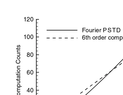
, where kxis the wavenumber rather than the meaning of sampling frequency in the temporal sequence. According to the Nyquist criteria, only 2 points-per-wavelength are required to obtain exact results [7]. This compares with other high-order finite difference methods, such as compact schemes, where typically 8 or more points-per-wavelength are required to meet the dispersion requirement.Compared to a typical high-order finite difference compact scheme, a potential performance limiting factor in applying the Fourier pseudospectral time-domain method is the relative deterioration in computation efficiency as larger grids are used. For a one-dimensional problem, the cost of performing discrete Fourier transform is proportional to O(m log2m), where m is the number of the discrete spatial points. A high-order finite difference method will typically require O(km) counts to obtain the derivative, where k is a constant for a specific scheme and generally has a value less than 6. Fig. 1 gives an illustration of the relative computation counts for one derivative scaled to the size of the computation domain. For a large computation domain, a pseudospectral time-domain method could potentially have lower computation efficiency than some high-order finite difference methods.
propagation of an open rotor [8, 9]. A summary of the present work is provided in Section 5.
2. GOVERNING EQUATIONS AND ALGORITHM 2.1. Governing Equations
The governing partial differential equations used to describe linear wave propagation phenomena in a uniform medium are given below. The one-dimensional convection equation takes the form of
(1)
The one-dimensional linearized Euler equations for acoustics wave propagation are given as:
(2)
(3)
The two-dimensional linearized Euler equations for acoustics wave propagation are given as:
(4)
(5)
∂ ′ ∂ +
∂ ′ ∂ =
v t
p
y 0,
∂ ′ ∂ +
∂ ′ ∂ =
u t
p
x 0,
∂ ′ ∂ +
∂ ′ ∂ =
p t
u
x 0.
∂ ′ ∂ +
∂ ′ ∂ =
u t
p
x 0,
∂ ′ ∂ +
∂ ′ ∂ =
u t
u
x 0.
Fourier P S T D 6th order compact 100
80
60
40
20
10 20
Computation Counts
120
0
0 30
[image:3.842.86.296.65.227.2]Grid points
(6)
In the above equations, t is the time, x and y are the Cartesian coordinates, u′and v′are velocity perturbations, and p′is the pressure perturbation. For the rest of the paper, the prime sign will be dropped for convenience. The fluid is modelled as a perfect gas, and all variables are nondimensionalised using a reference length L*, a reference sound
speed a*, and a reference density ρ*.
2.2. An Algorithm in the Pseudospectral Domain
With the assumption that the spatial domain is periodical, the one-dimensional convection equation, Eq. (1) can be transformed to:
(7)
where U–
(
kx, t)
is the pseudospectral pair for u(x,t), and kxis the wavenumber in the x direction. For this problem, an efficient algorithm can be employed to integrate Eq. (7) directly to the new time step t + k∆t as an ordinary differential equation to yield U–(
kx, t + k∆t)
, by using a suitable time-stepping scheme, e.g. a low-dissipation and low-dispersion Runge-Kutta scheme [10]. Temporal solution is obtained by applying an inverse Fourier transform to U–(
kx, t + k∆t)
, producing an updated solution u(x,t + k∆t).Following the same approach, the one-dimensional linear wave equations are transformed by the Fourier pseudospectral time-domain method to:
(8)
(9)
where P–
(
kx, t)
and U–(
kx, t)
are the pseudospectral pair for the pressure perturbation p(x,t) and velocity perturbation u(x,t) respectively.The transformed two-dimensional linear wave equations are as follows:
(10)
(11)
dV k k t
dt jk P k k t
x y
y x y
, ,
, , ,
(
)
+(
)
= 0dU k k t
dt jk P k k t
x y
x x y
, ,
, , ,
(
)
+(
)
= 0dP k t
dt jk U k t
x
x x
,
, ,
( )
+( )
= 0dU k t
dt jk P k t
x
x x
,
, ,
( )
+( )
= 0dU k t
dt jk U k t
x
x x
,
, ,
( )
+( )
=0
∂ ′ ∂ +
∂ ′ ∂ +
∂ ′ ∂ =
p t
u x
v
(12)
In Eqs. (10 – 12), and are the two-dimensional Fourier transforms of the velocity perturbations u(x,y,t) and v(x,y,t) and pressure perturbation p(x,y,t) respectively. Eqs. (8–12) could be stepped in the spectral domain directly as well. The above procedure can be applied to linear wave propagation equations with an underline mean flow to obtain and solve the transformed ordinary differential equations in pseudospectral domain.
2.3. Performance Analysis
The original algorithms of Fourier pseudospectral time domain method [6, 7] has the following form:
(13)
where DFT and IDFT denote forward and inverse discrete Fourier transforms. Other than the algorithm presented in section 2.2, this procedure is much more general. But the forward and inverse discrete Fourier transforms will have to be used at each time step to obtain the spatial derivatives.
As mentioned in section 2.2, some computational aeroacoustics applications could be solved as ordinary differential equations in the forms of Eqs. (7–12). For this type of problems, the approach adopted in this work is to apply discrete Fourier transform only at the start of the computation. The computation cost for the spatial derivatives at each time step is removed within this procedure.
In the case of a one-dimensional computational domain of m grid points, the fast Fourier transform algorithm requires operations in the order of O(m log2(m)), a typical low-dissipation and low-dispersion Runge-Kutta scheme requires operations in the order of O(4m), and a typical prefactored compact scheme’s computational complexity is in the order of O(6m) [11]. Consequently, it can be estimated that for each time step, the cost of a high-order finite difference method is in the order of O(10m), and the Fourier pseudospectral time domain method of the original algorithm (Eq. (13)) needs computation counts in the order of O(m log2 m + 4m). By comparison, the new computation procedure only requires operations in the order of O(4m). In fact it was acknowledged that for some applications the early algorithm for the Fourier pseudospectral time domain method had a comparable computing speed to an efficient finite difference scheme [12], even if a coarser grid was employed.
3. ISSUES AND SOLUTIONS
There are several issues in applying Fourier pseudospectral time domain method to computational aeroacoustics problems, such as resolution requirement and boundary
du
dt IDFT jk DFT f x
i
x i i
+ ( ( ( ))) = 0,
P k k t
(
x, y,)
U k k t
(
x, y,) (
, V k k tx, y,)
d P k k t
dt jk U k k t jk V k k t
x y
x x y y x y
, ,
, , , , ,
conditions. These are discussed in this section. The discussions apply to both algorithms of the pseudospectral time domain method.
3.1. Points-per-wavelength Requirement
For the Fourier pseudospectral time domain method a grid resolution of 2 points-per-wavelength is enough. Results in Fig. 2 presented demonstrate this point. In this exercise, the one-dimensional advection equation (Eq. (1)) with initial condition
of is solved. Two resolutions are employed: points-per-wavelength of 4 and 2. The computed results compare well with the analytical solutions.
3.2. Hard-wall Boundary Condition
The Fourier pseudospectral time domain method can be used to solve computational aeroacoustics problems effectively with high spatial resolution. The same property can be found in Schulten’s characteristic method [13]. However, the characteristic method could not solve problems with the presence of solid bodies and simulate the resulted sound reflection.
Based on the idea of generalized function [14], we now supply a hard-wall condition for the Fourier pseudospectral method. For simplicity the one-dimensional wave propagation Eqs. (2–3) are used in the derivation. We assume a stationary hard-wall condition on the left boundary of the computation domain at x = 0. The hard-wall condition suggests zero normal velocity at the wall. To ensure a correct velocity field, the following condition needs to be enforced
(14)
u( )0 u(0 ) u(0 ) .
2 0
= + + − =
uinit = 0 5e−4 2 x−50
2
. log( )( )
(a) (b)
0.6 0.6 0.7
0.4 0.3 0.2
89 90
x x
91 0.1
0 –0.1
Analytical solution
Fourier P S T D Fourier P S T D
u
0.6 0.6 0.7
0.4 0.3 0.2
89 90 91
0.1 0 –0.1
Analytical solution
u
88 92
[image:6.842.29.367.350.561.2]88 92
Figure 2. One-dimensional Gaussian pulse propagation with low
points-per-wavelength. (a) PPW = 4, ∆t / ∆x = 0.1, steps = 200. (b) PPW = 2, ∆t /
Eq. (3) can be re-casted using the idea of generalized derivative for functions with discontinuities [14] to
(15)
Eq. (15) can be transferred by a discrete Fourier transform to
(16)
where u(0+, t) is approximated by u(0,t), which is obtained from an inverse discrete Fourier transform operating on in each step.
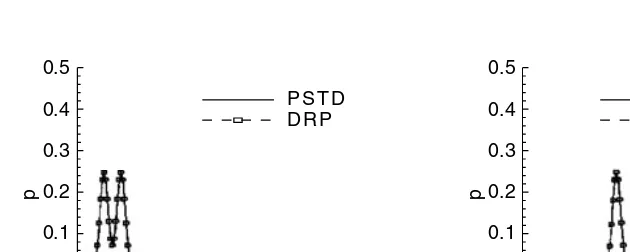
An example of the application with hard-wall condition is shown in Fig. 3, where a one-dimensional wave is reflected from a hard wall at the left boundary. The initial
condition is a Gaussian pulse defined by Eqs. (8) and (16) are used to obtain the solutions. Comparison is made with a fourth-order dispersion-relation-preserving (DRP) scheme [15]. In the most part, two results agree well, but a rewrap wave appears when the Fourier pseudospectral time domain method is used. It is generated by the periodical boundary condition and can be absorbed by the technique described in the next section.
3.3. Absorbing Condition for Rewrap Waves
The original Fourier pseudospectral time domain method works for problems with periodical boundaries. When the periodical assumption is not satisfied, wave rewrap phenomenon will appear and contaminate the solutions in the computation domain. In this work, an explicit form of buffer zone techniques [16] is applied to absorb the reflected waves. The buffer zone technique works in the spatial domain, and
pinit = 0 5e− 2 x=20 9 uinit = 0
2
. log( )( ) / , .
U k t
( )
x,∂
( )
∂ +
( )
++ =
P k t
t jk U k t
u t
x
x
x x
,
, 2 0( , ) 0,
∆ ∂
∂ + ∂
∂ +
[
+ − −]
=p x t t
u x t
x u t u t x
( , ) ( , )
(0 , ) (0 , ) δ( ) 0.
(a) (b)
0.5
0.4
0.3
0.2
0.1
0
50 0
p
x
100 150 200
–0.1 0.5
0.4
0.3
0.2
0.1
0
50 0
p
x
100 150 200
–0.1
P S T D D R P P S T D
[image:7.842.42.357.63.189.2]D R P
Figure 3. One-dimensional Gaussian pulse reflected by a left hard-wall; without
consequently the new algorithm for the Fourier pseudospectral time domain method requires more operation counts. The exact number depends on the width of the buffer zone; there is therefore a trade-off between memory and speed.
In the implementation, the solution vector is explicitly damped after every several time step by
(17)
where is the solution vector computed after regular time steps and F0is the target solution. The damping coefficient, σ, varies according to the function,
(18)
where L is the width of the buffer zone, x is the distance from the inner boundary of the buffer zone and σmaxand βare set to 1.0 and 3.0 respectively. In this work the target solution F0is set to 0.
4. APPLICATIONS TO BENCHMARK PROBLEMS
The aforementioned method is applied to two benchmark test cases. Results and discussions are given here. In the first case, a two-dimensional Gaussian pulse propagation problem with hard-wall and absorbing boundaries was computed, employing temporal integration directly on pseudospectral space. In the second case, the algorithm in the form of Eq. (13) was used to solve for an open rotor problem with nonlinear terms.
4.1. Wave Propagation and Reflection
This case is the first problem of category 4 that is defined at first computational aeroacoustics workshop [8]. The initial condition is a Gaussian acoustic pulse given by:
(19)
uinit = 0, (20)
vinit = 0. (21)
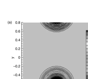
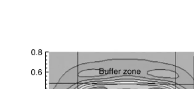
Eqs. (10–12) are used to solve the problem. ∆t / ∆x is set to 0.5. Results are presented in Fig. 4. The hard-wall boundary condition on the bottom boundary appears to have reproduced the reflected waves off the bottom wall. In this exercise, the length of the buffer zone is set to 10 grid points. In the current computation, the buffer zone is not updated at each time step. Instead, the solutions inside the buffer zone are updated at regular step intervals, e.g. once every 2 or 4 steps, to save computing time furthermore. The algorithm employed for this exercise can be found in the appendix.
pinit e
x y
= −log( ) + +( . )/ .
,
2 2 0 62 0 006
σ σ
β ( )x max
x L
L
= 1 − −
F( ,x t + ∆t)
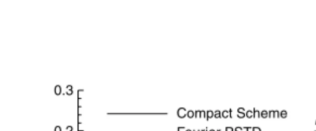
The pressure distribution along the x = 0 axis is given in Fig. 5 and compared with the prediction given by a prefactored compact scheme [11]. The computing time t and L2error against to an analytical solution of linearized Euler equations [15] are listed in Table 1, where the spatial resolution is low, from around 3 points-per-wavelength to 12 points-per-wavelength. 0.6 0.4 0.2 0 –0.2 –0.4 –0.6
–0.6 –0.4 –0.2 0 0.2 0.4 0.6 0.8 0.32 0.26 0.20 0.14 0.08 0.02 –0.04 –0.10 0.6 0.4 0.2 0 –0.2 –0.4 –0.6
–0.6 –0.4 –0.2 0 0.2 0.4 0.6 0.8 P 0.32 0.26 0.20 0.14 0.08 0.02 –0.04 –0.10 P 0.6 0.4 0.2 0 –0.2 –0.4 –0.6
–0.8 –0.6 –0.4 –0.2 0 0.2 0.4 0.6 0.8 1 0.32 0.26 0.20 0.14 0.08 0.02 –0.04 –0.10 0.6 0.4 0.2 0 –0.2 –0.4 –0.6
–0.6 –0.4 –0.2 0 0.2 0.4 0.6 0.8 P 0.32 0.26 0.20 0.14 0.08 0.02 –0.04 –0.10 P x 0.8
Buffer zone Buffer zone
Buff er z one Buff er z one Buff er z one Buff er z one –0.8 y 0.8 –0.8 y
–0.8 1
x
–0.8 1
x 0.8
–0.8
y
–0.8 1
[image:9.842.25.367.69.375.2]x 0.8 –0.8 y (a) (b) (c) (d)
Figure 4. The propagation of a two-dimensional Gaussian pulse. (a) t = 0.25,
without buffer zone. (b) t = 0.4, without buffer zone. (c) t = 0.25, buffer zone. (d) t = 0.4, buffer zone.
Table 1. Computing time t and L2error of the first benchmark problem
Schemes 16 ××16 64 ××64
It has been discovered that with Fourier pseudospectral time domain method, if a buffer zone is not applied, wave rewraping will contaminate the solutions. However, if the rewrap wave is not considered in computing L2 errors over two grids, they are 0.0107 and 0.00083 correspondingly, indicating the pseudospectral method is actually more exact than the compact scheme. Fig. 4(c – d) and Fig. 5(b) illustrate that a buffer zone keeps removing the rewrap wave. The agreement is generally good as well. However, the buffer zone affects the spectra of the solution near the hard wall as it absorbs the rewrap wave. It has been found that this difference will remain stable as the solution develops. L2 error results in Table 1 also indicate that the buffer zone does affect the accuracy of the Fourier pseudospectral method. But for the majority of the domain, there are no significant differences in the solutions (see Fig. 5(b)). Fig. 6 also presents a comparison between the Fourier pseudospectral time domain method and the prefactored compact scheme after 110 time iterations.
In terms of computation efficiency, the Fourier pseudospectral method, with or without a buffer zone, represents a saving of up to 200% compared with the prefactored compact scheme.
4.2. Open Rotor
The second test case is that of the open rotor noise defined in category 2 benchmark problem at third computational aeroacoustics workshop [9]. It has nonlinear source terms and could not be described in pseudospectral domain accordingly. The simplified algorithm using a temporal stepping directly on Eqs. (7–12) is not applicable here. Consequently the original algorithm in the form of Eq. (13) is used to show the effectiveness of the Fourier pseudospectral method for general problems.
The governing equations in cylindrical coordinates and the definitions of the problem are as follows:
(a) (b)
Compact Scheme 0.2
0
0 0.2 0.4 0.6 0.1
–0.1
–0.2 –0.4
Fourier PSTD
0.8 –0.6
y 0.3
–0.2
p
Compact Scheme 0.2
0
0 0.2 0.1
–0.1
–0.2 –0.4 –0.6
Fourier PSTD
0.4 –0.8
y 0.3
–0.2
[image:10.842.41.358.63.195.2]p
Figure 5. A comparison of two-dimensional Gaussian pulse propagation predicted
(22)
(23)
(24)
(25)
where x is the axial coordinate, r the radial coordinate, and Φthe azimuthal angle. u,v,w are the velocity perturbations in the x,r,Φ directions respectively, and p is the pressure perturbation. The nonlinear terms are defined as:
(26)
Sr= 0, (27)
(28)
(29)
~
S r x S x J r r ,
r x M MN ( , ) ( ) ( ), , = ≤ > λ 0 1 1
S r x t
S r x t
S r x
S r x e
x x
iM t
Φ Φ Φ Φ Ω
Φ
( , , , ) ( , , , ) Re
( , ) ( , ) , ( ) = −
S x e x
( ) = −(ln )(2 10 )2,
∂ ∂ + ∂ ∂ + ∂ ∂ + ∂ ∂ = p t u x r ur r r w 1 1 0 Φ , ∂ ∂ = − ∂ ∂ + w t r u S 1
Φ Φ,
∂ ∂ = − ∂ ∂ + v t p
r Sr,
∂ ∂ = − ∂ ∂ + u t p
x Sx,
0.6 P 0.10 0.08 0.06 0.04 0.02 Buffer zone
Buffer zone Buffer zone
Buffer zone Buffer zone
Buffer zone 0.00 –0.02 –0.04 –0.06 –0.08 –0.10 0.2
0.2 0.4 0.6 0.8 –0.2
–0.4
–0.6
–0.6 –0.4 –0.2 0.4 0 0 x 1 –0.8 0.8 y –0.8 0.6 P 0.100 0.080 0.060 0.040 0.020 0.000 –0.020 –0.040 –0.060 –0.080 –0.100 0.2
0.2 0.4 0.6 0.8 –0.2
–0.4
–0.6
[image:11.842.45.360.69.214.2]–0.6 –0.4 –0.2 0.4 0 0 x 1 –0.8 0.8 y –0.8 (a) (b)
Figure 6. A comparison of two-dimensional Gaussian pulse propagation after 110
time steps. Pressure contours. (a) Fourier PSTD method. (b) 6thcompact
(30)
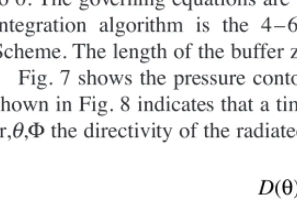
where JMis the M th-order Bessel function of the first kind, λMNis the N th root of J′M or J′M(λMN) = 0. The parameters are M = 8,N = 1,λ8,1 = 9.64742 and Ω= 0.85. The computation domain covers [–5,5] in the axial direction and the radial direction. The size of the grid ∆x and the time step ∆t obey the relation ∆t /∆x = 0.5. Φ is set to 0. The governing equations are solved by the algorithm given in Eq. (13). The time integration algorithm is the 4 – 6 low-dissipation and low-dispersion Runge-Kutta Scheme. The length of the buffer zone is 15 grid points.
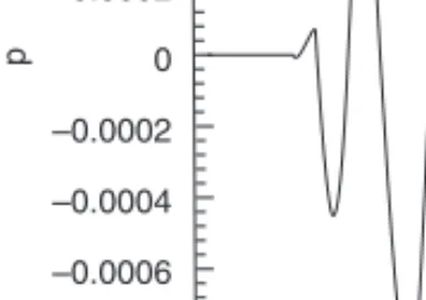
Fig. 7 shows the pressure contours after 80 time steps. The monitored time history shown in Fig. 8 indicates that a time periodic state is reached. In spherical coordinates (r,θ,Φthe directivity of the radiated sound is defined as:
where r, Φand θare radius, azimuthal angle and polor angle respectively.
is the time average of P2(r,Φ,θ,t). The predicted directivity of the rotor noise is
compared with an analytical solution [9] in Fig. 9. Here the radius r is set to 3. Although the radius is not large enough, the two results still agree well. The computing time t and error Err of DRP, Compact and the Fourier pseudospectral schemes are compared in Table 2, where
Err D i Danalytical i
i
=
( )
− ∈ −
=
∑
θ ( ) ,θ θ 20 160 .1 8
P r2
( ,Φ θ, )
D r P r
r
( )θ = lim ( , , )θ →∞
2 2 Φ
~
S r x S x rJ r r ,
r
M MN
Φ( , )
( ) ( ), ,
= ≤
>
λ
0
1 1
4
3
2
1
P 0.0005
–0.0015
–0.0035
–0.0055
–0.0075
–0.0095
–0.0115
–0.0135
–5 –4 –3 –2 –1 0 1 2 3 4 5
x
5
0
[image:12.842.52.346.357.577.2]r
In this case, the pseudospectral method is only employed to obtain the spatial differential terms. The numerical error affiliated with the buffer zone and the slip wall boundary condition does not exist. Consequently, results in Table 2 indicate that the Fourier pseudospectral time domain method can obtain much more accurate solutions
0
4 6 8
0.0006
0.0004
0.0002
–0.0002
–0.0004
–0.0006
p
0.0008
–0.0008
2
t
[image:13.842.44.352.63.217.2]10
Figure 8. Pressure time history generated by an open rotor at (x = – 0.1, r = 1.9).
6E-06
7E-06 Fourier PSTD
Analytical solution
5E-06
3E-06 4E-06
2E-06
1E-06
0
0 20 40 60 80 100 120 140 160 180
D
[image:13.842.99.293.258.394.2]θ
Figure 9. Directivity of an open rotor acoustic radiation, r = 3.0; a comparison
between prediction and analytical solution. θis the polar angle.
Table 2. Computing time t and L1error of the second
benchmark problem
Schemes 100××100 200××200
DRP t = 21.6s, Err = 7.9e–6 t = 186s, Err = 6.1e–6
Compact t = 34.1s, Err = 6.8e–6 t = 557s, Err = 5.9e–6
with smaller points-per-wavelength numbers. It is also much more efficient than other high-order finite difference methods.
5. CONCLUSIONS
The Fourier pseudospectral time domain method has been applied to some benchmark problems pertinent to computational aeroacoustics. For linear wave propagation problems, a new algorithm has been developed and tested. The updated time stepping method relaxes time stepping restrictions. A hard-wall boundary condition is supplied for simple geometry and has been validated. Combined with the buffer zone technique to reduce contamination due to wave rewrap, the algorithm becomes fully-fledged to some linear wave propagation problems. For general problems with nonlinear terms, the original algorithm of the Fourier pseudospectral time domain method is shown to be an alternative to high-order finite difference methods.
ACKNOWLEDGMENTS
Xun Huang is supported by a scholarship from the School of Engineering Sciences, University of Southampton.
REFERENCES
[1] Kosloff, D., and Kosloff, R., A fourier method solution for the time dependent Schrödinger equation as a tool in molecular dynamics, Journal of Computational Physics, 1983, 52(1), 35–53.
[2] Driscoll, T. A., and Fornberg, B., A block pseudospectral method for Maxwell’s equations, Journal of Computational Physics, 1998, 140(1), 47–65.
[3] Wang, Y., and Takenaka, H., A multidomain approach of the Fourier pseudospectral method using discontinuous grid for elastic wave modeling, Earth Planets Space, 2001, 53, 149–158.
[4] Liu, Q. H., PML, and PSTD algorithm for arbitrary lossy anisotropic media, IEEE Microwave And Guided Wave Letters, 1999, 9(2), 48–50.
[5] Fornberg, B., A Practical Guide to Pseudospectral Methods, Cambridge University Press, 1998.
[6] Liu Q. H., and Zhao, G., Review of PSTD methods for transient electromagnetics, International J. Numerical Modeling, 2004, 17, 299–323 .
[7] Liu, Q. H., The PSTD algorithm: A time-domain method requiring only two cells per wavelength, Microwave and Optical Technology Letters, 1997, 15(3), 158–165. [8] Hardin, J. C., Ristorcelli, J. R, and Tam, C. K. W., (Eds.), ICASE/LaRC Workshop
on Benchmark Problems in Computational Aeroacoustics, NASA CP-3300, NASA, 1995.
[9] Milo, D. D., (Eds.), Third computational aeroacoustics (CAA) workshop on benchmark problems, Technical Report NASA CP-2000-209790, NASA, 2000. [10] Hu, F. Q., Hussaini, M. Y., and Manthey, J., Low-dissipation and low-dispersion
[11] Ashcroft, G., and Zhang, X., Optimized prefactored compact schemes. Journal of Computational Physics, 2003, 190(2), 459–477.
[12] He, J. P., Shen, L. F., Zhang, Q., and He, S. L., A pseudospectral time-domain algorithm for calculating the band structure of a two-dimensional photonic crystal, Chinese Phys. Lett., 2002, 19(4), 507–510.
[13] Schulten, J., On the use of characteristics in CAA, AIAA Paper 2002-2584, 2002. [14] Farassat, F., Generalized functions and kirchhoff formulas, AIAA Paper 96-1705,
1996.
[15] Tam, C. K. W., and Webb, J. C., Dispersion-relation-preserving finite difference schemes for computational acoustics, Journal of Computational Physics, 1993, 107(2), 262–281.
APPENDIX: SAMPLE CODE FOR TWO-DIMENSIONAL WAVE EQUATIONS
function [x,y,u,v,p,clocka,clockb]=Wave2DFreqBCRewrap2(dx,ntsteps)
%******************************************************************% % x,y:grid; u,v,p:velocity and pressure;
% dx:spatial step; ntsteps:operation steps;
%******************************************************************% RK_dt=dx*0.3; %CFL, RK_dt=0.1, 0.05,and 0.025 have been tested before.
[x,y]=meshgrid(–0.8+dx:dx:0.8); %make grids. dimen=size(x); dimen=dimen(1);
u=0*x;v=0*x;p=exp(-log(2.0)*(x.^2+(y+0.6).^2)/0.006); Uifft=u;Vifft=v;
omegaT1=[0.25,0.33333333333,0.5,1.0]*RK_dt; %Runge-Kutta coef inv_dimen=1/dimen; inv_dx=1/dx;max_half=dimen/2;
tmp=-sqrt(-1)*2*pi*inv_dimen*inv_dx;
Vall=zeros(1,dimen); %Vall is used for hard wall reflection. totalstep=0; clocka=clock;
P=fft2(p,dimen,dimen);U=fft2(u,dimen,dimen);V=fft2(v,dimen,dimen); U=fftshift(U);V=fftshift(V);P=fftshift(P); P0=P;U0=U;V0=V;
while(totalstep<ntsteps) for s=1:1:1
for subit=1:1:4 for m=1:1:dimen
for n=1:1:dimen
Tmp_Px=tmp*(n–max_half–1)*P(m,n); Tmp_Py=tmp*(m–max_half–1)*P(m,n); Tmp_Ux=tmp*(n–max_half–1)*U(m,n);
Tmp_Vy=tmp*(m–max_half–1)*V(m,n) –2*Vall(1,n)*inv_dx; U(m,n)=U0(m,n) + Tmp_Px*omegaT1(subit);
V(m,n)=V0(m,n) + Tmp_Py*omegaT1(subit);
P(m,n)=P0(m,n) + (Tmp_Ux+Tmp_Vy)*omegaT1(subit); end
end
Vifft=ifft2(V);Vall=fft(Vifft(1,:)); end
U0=U;V0=V;P0=P;totalstep=totalstep+1 %Update all end
end