Zsolt darvas (zsolt. [email protected]) is a Senior Fellow at Bruegel and Corvinus University of Budapest
This Policy Contribution was prepared for the Nomura Foundation’s Macro Economy Research Conference: ‘Monetary Policy Normalization Ten Years after the Great Recession’, 24 October 2018, Tokyo. Financial support from the Nomura Foundation is gratefully acknowledged. The author thanks conference participants and Bruegel colleagues for useful comments and suggestions, and Bowen Call, Antoine Mathieu Collin and Catarina Midoes for excellent research assistance.
Executive summary
We consider the lessons of the recent monetary policy normalisation experiences of Sweden, the United States and the United Kingdom, and analyse the European Central Bank’s forecast-ing track record and possible factors that might explain the forecast errors. From this analysis, we draw the following main conclusions:
1. Monetary tightening involves major risks when the evidence of an improved inflation outlook is not sufficiently strong; it is better to err on the side of a possible inflation overshoot after a long period of undershooting;
2. Inadequate forward guidance can cause market turbulence;
3. Market participants might disregard forward guidance after large systematic forecast errors;
4. Terminating net asset purchases might not increase long-term rates, though it might have an impact on other asset prices because of the lack of portfolio rebalancing;
5. The ECB has made huge and systematic forecasting errors in the past five years, indicating that some of the behavioural relationships in ECB forecasting models are mis-specified. The ECB is not the only institution to suffer from incorrect forecasts and there should be broader debate on forecasting practices. However, the ECB’s forecast errors and its inability to lift core inflation above 1 percent have major implications;
6. Market-based inflation expectations have already started to fall in the euro area,
suggesting that the trust has weakened in the ECB’s ability to reach its inflation aim of the below but close to two percent over the medium term;
7. More time is needed to see if the forecasting failures of the past five years were driven by factors whose impact will gradually fade away, or if the ECB’s ability to lift core inflation has been compromised;
8. In the meantime, a very cautious approach to monetary policy normalisation is
recommended. A rate increase is only recommended after a significant increase in actual core inflation. This intention should be made clear in the ECB’s forward guidance; 9. If forecasting failures continue and core inflation does not approach two percent, the
ECB’s credibility could be undermined, making necessary a discussion on either the deployment of new tools to influence core inflation, or a possible revision of the ECB’s inflation goal;
10. In the new ‘normal’ the natural rate of interest might remain low, and thereby central bank balance sheet policies will likely became part of the regular toolkit;
11. Monetary policy tools are ill-suited to address financial stability concerns in general, especially in the euro area. Financial stability concerns should not play a role in
monetary policy normalisation. Instead, country-specific macroprudential policy should complement micro-prudential supervision and regulation.
Policy Contribution
Issue n˚24 | December 2018
Forecast errors and
monetary policy
normalisation in the euro area
1 Motivation
[image:2.595.186.518.213.438.2]The global financial and economic crisis, which intensified after the collapse of Lehman Brothers in September 2008, has led to the deepest economic contraction in many advanced countries since the second world war. Unusual economic circumstances have triggered unu-sual monetary policy measures. Central banks quickly cut their interest rates close to zero in 2008-09 – joining the Bank of Japan, which has long implemented a close-to-zero interest rate policy (Figure 1).
Figure 1: One-week interbank interest rates (%), 2 January 2000 – 7 December 2018
-2 -1 0 1 2 3 4 5 6 7
20
00
20
01
20
02
20
03
20
04
20
05
20
06
20
07
20
08
20
09
20
10
20
11
20
12
20
13
20
14
20
15
20
16
20
17
20
18
US dollar
British pound sterling Japanese yen Euro
Swedish krona Swiss franc
Source: Bruegel based on Bloomberg and Sveriges Riksbank. Note: We show the 1-week interbank rates and not central banks’ interest rates, because for some central banks the importance of certain rates changed (eg for the European Central Bank, the main refinancing operations (MRO) interest rate was the main determinant of short-term market rates before 2008, but since then the ECB’s deposit rate has been the main determinant). STIBOR (Stockholm Interbank Offered Rate) for the Swedish krona, LIBOR (London Interbank Offered Rate) for all other currencies.
Zero has long been considered a lower bound for interest rates, and close-to-zero rates thus gave rise to the discussion about the ‘zero lower bound’ (ZLB). The rationale for the ZLB is that a negative interest rate might be ineffective if agents do not want to pay a ‘fee’ (ie the negative interest rate) for holding deposits. Agents would instead hoard cash1. Since
hold-ing cash involves storage costs and risks of destruction and theft, the effective lower bound should be lower than zero, yet in 2008-09 central banks had not (yet) opted for negative inter-est rates. Instead, several advanced country central banks adopted various other monetary policy measures, which aimed to ease monetary conditions further. These measures included large-scale asset purchases, such as government bonds and various private sector or agency securities (called ‘quantitative easing’) and large-scale liquidity provision measures, through which banks were able to obtain loans from the central bank for longer maturities and at more attractive terms than in the pre-crisis period. Again, the Bank of Japan was a forerun-ner in the adoption of quantitative easing measures even before the crisis, in 2001-06. Some other central banks, most notably the Swiss National Bank and the Danish National Bank,
purchased large amounts of foreign currency to prevent the appreciation of the exchange rate of their currencies. These measures boosted the size of central bank balance sheets to unforeseen levels, at least since the second world war (Figure 2). While there were sizeable differences in central banks’ pre-crisis balance sheet sizes, the differences became even more striking after 2008.
Figure 2: Central bank balance sheets (% GDP), January 2006 – August 2018
0 20 40 60 80 100 120 140
20
06
20
07
20
08
20
09
20
10
20
11
20
12
20
13
20
14
20
15
20
16
20
17
20
18
Swiss National Bank
Bank of Japan
European Central Bank
Bank of England Federal Reserve
Sveriges Riksbank
Source: Bruegel based on balance sheet data: Federal Reserve Bank of St. Louis (BoJ: JPNASSETS, ECB: ECBASSETS, FED: WALCL, BoE: UKASSETS), Bank of England (RPQB75A), Swiss National Bank ([email protected]{T0}) and Sveriges Riksbank (The Riksbank’s assets and liabilities weekly report); GDP: IMF (WEO), Eurostat [nama_10_gdp], Swiss National Bank ([email protected]{WMF,BBIP}) and Statistics Sweden quarterly accounts (GDP at market prices).
As the economic outlook improves and inflation gradually increases, the key questions are when and how these historically unprecedented monetary policy measures should be normalised, and to what levels. In fact, Figure 1 shows that euro and Swedish short-term interest rates started to increase from mid-2010, reflecting monetary tightening by the Euro-pean Central Bank and the Sveriges Riksbank. In both currency areas, the tightening proved to be short-lived. An even more significant period of monetary policy easing has followed, suggesting that the mid-2010 normalisation attempts were premature. We will scrutinise these episodes.
More recently, the Federal Reserve started to take several steps toward monetary policy normalisation, following the sequence: 1) gradual reduction in net asset purchases; 2) stopping net asset purchases (with maturing asset holdings reinvested to keep the stock of assets unchanged); 3) increasing the interest rate a few times; 4) gradually reducing reinvestments to allow asset holdings to shrink, while continuing the gradual process of increasing the interest rate. The key dates for the US in relation to the third and last round of quantitative easing were December 2013 for stage 1, September 2014 for stage 2, December 2015 for stage 3 and September 2017 for stage 4.
Other central banks have followed this sequence. The Bank of England started a nor-malisation process in 2012, but the Brexit referendum in 2016 triggered a new round of quantitative easing. Since economic developments were more favourable than predicted in the immediate aftermath of the referendum and inflation started to accelerate, partly because of the significant depreciation of the pound sterling, the Bank of England started a normalisation process by increasing the base rate by 25 basis points in November 2017 and then again in August 2018, thereby reaching stage 3.
to lift interest rates, though asset purchases have ended in Sweden and are expected to end by end-2018 in the euro area. The Bank of Japan has not yet announced a reduction in the monthly amount of asset purchases, though Shirai (2018) noticed that there has been a reduction.
This Policy Contribution assesses the monetary policy normalisation process from the perspective of the euro area. We answer, for the euro area, the questions of when and how to normalise monetary policy measures2, questions that are ultimately linked to achieving
the ECB’s inflationary objective.
We first analyse certain problems that characterised the monetary policy normalisa-tion processes in Sweden, the United States and the United Kingdom. We then scrutinise the possible ‘new normal’ for monetary policy in terms of interest rates and central bank balance sheets. Third, we analyse the track record of ECB inflation forecasts and assess the factors that might have contributed to forecast errors. And fourth, we briefly assess whether financial stability concerns should play a role in monetary policy normalisation.
2 Lessons from monetary policy exit
mistakes in Sweden, the US and the UK
The central banks of Sweden, the United States and the United Kingdom adopted certain monetary policy normalisation measures, leading to adverse market reactions. These ep-isodes offer valuable lessons for monetary policy normalisation by other central banks. In Sweden, a premature exit started in summer 2010, followed by massive monetary policy easing. The examples from the United States (late 2012 to summer 2013) and the United Kingdom (summer 2013 to summer 2014) share many similarities with each other. In both the US and UK, the future interest rate increase was initially linked to a certain level of unemployment and was then de-linked when the unemployment rate fell. Other com-munication and forward guidance problems suggesting a near-term interest rate increase have contributed to a significant but temporary increase in long-maturity government bond yields, followed by an even more significant bond yield decline.
2.1 Sweden: premature exit followed by massive monetary policy easing
Sweden provides an example of premature exit from expansive monetary policies, which then had to be reversed and were followed by an even more significant monetary easing. When the global financial crisis intensified after the collapse of Lehman Brothers in Sep-tember 2008, the Sveriges Riksbank, Sweden’s central bank, cut its main monetary policy rate. The so-called repo rate (at which banks can borrow or deposit funds at the Riksbank for a period of seven days) was cut from 4.75 percent in October 2008 to 0.25 percent in July 2009 (Figure 3). However, between July 2010 and July 2011, the Riksbank increased its main policy rate from 0.25 percent to 2 percent in seven steps, largely to address finan-cial stability concerns (Svensson, 2014). The rapid 2010 recovery from the deep 2009 recession (Figure 4) probably gave the Riksbank confidence to pursue monetary policy tightening.
Figure 3: Swedish interest rates (%), 2 January 2008 – 7 December 2018
Source: Sveriges Riksbank, https://www.riksbank.se/en-gb/statistics/search-interest--exchange-rates/. Note: The repo rate has been the Riksbank’s policy rate since 1994. The repo rate is the rate of interest at which banks can borrow or deposit funds at the Riksbank for a period of seven days. In addition, the Riksbank has an overnight deposit facility, which has an interest rate 0.75 percentage points lower than the repo rate, and an overnight borrowing facility, which has a rate 0.75 percentage points higher than the repo rate.
Sweden is an open economy and external shocks, such as the global financial crisis which originated in the US, and the double-dip recession in the euro area, likely played major roles in the economic development of Sweden. Yet according to Svensson (2014), the premature monetary policy tightening also contributed to macroeconomic fluctuations: it led to high costs in terms of excessively low inflation, overly high unemployment and a higher real debt burden for households. Inflation fell quickly after 2011 and even in 2014 was close to zero, well below the 2 percent target (Figure 4). The unemployment rate also fell less rapidly than under a counterfactual scenario of continued low interest rates, suggesting that the premature monetary tightening pushed up the unemployment rate by about 2 percentage points for several years (Svensson, 2014).
Figure 4: Some key macroeconomic indicators of Sweden, 2000Q1 – 2018Q3
Sources: Bruegel based on Eurostat datasets: ‘GDP and main components (output, expenditure and income) [namq_10_gdp]’, ‘Unem-ployment by sex and age - quarterly average [une_rt_q]’, ‘HICP (2015 = 100) - monthly data (annual rate of change) [prc_hicp_manr]’, and ‘House price index (2015 = 100) - quarterly data [prc_hpi_q]’. Note: percent change compared to the same quarter of the previous except for the unemployment, which is in percent of the labour force.
-1 0 1 2 3 4 5 20 08 20 09 20 10 20 11 20 12 20 13 20 14 20 15 20 16 20 17 20 18 Repo rate 3-month treasury bill rate 10-year government bond yield QE s ta rts QE e nd s pu rc ha se s in cr ea se d pu rc ha se s re du ce d pu rc ha se s re du ce d pu rc ha se s re du ce d -8 -6 -4 -2 0 2 4 6 8 10 12 14 16 20 00 20 01 20 02 20 03 20 04 20 05 20 06 20 07 20 08 20 09 20 10 20 11 20 12 20 13 20 14 20 15 20 16 20 17 20 18
GDP growth All items inflation Core inflation
[image:5.595.183.486.497.706.2]Ultimately, low inflation forced the Riksbank to cut rates to even lower levels: the repo rate was cut from 2 percent in July 2011 to -0.5 percent in February 2016. Moreover, the Riksbank also started to purchase Swedish government bonds for monetary policy purposes, starting in April 2015 with Swedish Krona 40-45 billion a month, increased to kr65 billion per month in October of the same year. However, although the Riksbank initially aimed to ward off the threat to financial stability of household over-indebtedness, the household debt-to-income ratio was not affected by the 2010-11 policy of tightening and in fact the ratio continued to increase in real terms, partly because of the very low inflation rates.
[image:6.595.184.528.312.545.2]Furthermore, Riksbank interest rate guidance since 2011 turned out to have been inad-equate. The Riksbank is among the few central banks to publish numerical forecasts for its main monetary policy rate (along with a confidence band). Only the 2010-11 tightening was in line with forecasts; Riksbank interest rate forecasts made both before and especially after this period, which predicted increases in the Riksbank’s own interest rate, proved to be sys-tematically wrong (Figure 5). These systematic forecast errors call into question the usefulness of the publication of interest rate forecasts.
Figure 5: The Riksbank’s repo rate: actual and Riksbank forecasts (%), 2006Q1–
2021Q3
Source: Bruegel based on various Sveriges Riksbank monetary policy reports. Note: the actual rate is the thick red line, while the other lines show the Riksbank forecasts.
Gradual tapering of net government bond purchases started in April 2016 with actual net purchases stopped at the end of 2017. Yet the Riksbank still reinvests maturing bonds to keep the stock of its government bond holdings unchanged, because “the Riksbank’s strategy for a gradual normalisation of monetary policy involves continuing to reinvest principal payments in
the government bond portfolio for a while even after repo rate rises have begun” (Riksbank, 2018).
Therefore, even though both the headline and the core inflation rate reached the two per-cent target in early 2017 (Figure 4), the Riksbank remained much more cautious and has not yet tightened monetary conditions. This cautious approach has been justified, given that core inflation had fallen back to 1.5 percent by mid-2018.
It is also important to note that the 10-year government bond yield has not increased with the tapering and eventual stop of quantitative easing, but has largely remained in the 0.5-1 percent range, apart from a brief episode in the autumn of 2016 when it fell close to zero (Figure 3). The government bond yield is well below pre-crisis values. The relative stability of the 10-year
-1 0 1 2 3 4 5 6
20
06
20
07
20
08
20
09
20
10
20
11
20
12
20
13
20
14
20
15
20
16
20
17
20
18
20
19
20
20
20
government bond yield is also in contrast to the Riksbank’s own prediction of a rate increase (Figure 5)3, suggesting the Riksbank’s forward guidance is ineffective. We cannot exclude the
hypothesis that market participants disregard the Riksbank’s forward guidance because of the massive and systematic forecast errors made in the past.
Anyhow, the Swedish experience highlights that stopping net asset purchases would not necessarily lead to higher long-term interest rates.
These experiences offer important lessons to the European Central Bank:
• Premature tightening (when the evidence of an improved inflation outlook is not suf-ficiently strong) should be avoided; it is better to err on the side of a possible inflation overshoot after a long period of undershooting;
• A cautious approach to interest rate increases and balance sheet reductions could be justified when the inflation outlook is uncertain;
• Market participants might disregard forward guidance after large systematic forecast errors;
• Stopping net asset purchases might not lead to an increase in the long-term interest rate.
2.2 Federal Reserve: ‘taper tantrum’ unnecessarily pushed-up the
10-year yield
As the US economy gradually recovered from the deep recession of 2008-09, in December 2012 the Federal Reserve introduced a new way of forward guidance to communicate its ex-pected policy intentions by stating a particular value of the unemployment rate, which would trigger monetary policy changes. The Federal Market Open Committee (FOMC) said it “ an-ticipates that this exceptionally low range for the federal funds rate will be appropriate at least as long as the unemployment rate remains above 6-1/2 percent, inflation between one and two years ahead is projected to be no more than a half percentage point above the Committee’s 2
percent longer-run goal, and longer-term inflation expectations continue to be well anchored”4.
As Whelan (2018) noted, the clear majority of FOMC members believed at that time that the 6.5 percent unemployment rate would not be reached until 2015.
In early 2013, the unemployment rate fell to 7.5 percent, nearing the 6.5 percent threshold. The FOMC started to discuss tapering (ie reducing the amount of asset purchases) of the third round of quantitative easing in early May 2013. Such a discussion, along with the fall in the unemployment rate towards the 6.5 percent threshold, raised market expectations of a federal funds rate increase. The expected increase in short-term interest rates led to a rather signifi-cant increase in the 10-year yield, which increased from 1.7 percent in May 2013 to 3 percent a few months later (Figure 6), leading to a far greater tightening of financing conditions than the Fed had intended.
Eventually, the unemployment rate fell below 6.5 percent, but inflation did not pick up (Figure 7) and economic growth was somewhat weaker than expected. Thus, the Federal Reserve did not increase rates until December 2015 (when the unemployment rate was down to 5 percent). Later, the 10-year government bond yield fell back even below 1.7 percent, despite the actual tapering and ending of asset purchases and the first increase in December 2015 in the federal funds rate. The median of the longer-term federal funds rate projections of FOMC members did not change between June 2014 and June 2015, and therefore the publi-cation of these projections is unlikely to have contributed to the significant fall in the 10-year government bond yield in this period. Yet in the subsequent year, from June 2015 to June 2016, this median longer-run expectation fell from 3.75 percent to 3 percent, which might
3 According to the hypothesis of the term structure of interest rates, the long-maturity interest rate is the average of the current and expected short maturity interest rates plus possibly a term premium. Thereby, an expected increase in the short-term interest rate should lead to increases in longer maturity interest rates.
have impacted government bond yield developments. The US experience was thus similar to the Swedish experience and suggests that stopping net asset purchases does not necessarily lead to a higher long-term interest rate.
Figure 6: US interest rates (%), 2 January 2000 – 6 December 2018
Source: Bruegel based on Federal Reserve; effective federal funds rate: H15/RIFSPFF_N.B; 10-year government bond yield: H15/RIFLG-FCY10_N.B; federal funds rate projections: collected from Projections Materials from https://www.federalreserve.gov/monetarypolicy/ fomccalendars.htm and SEP - Accessible material from https://www.federalreserve.gov/monetarypolicy/fomc_historical_year.htm . Note: The federal funds rate projections correspond to policymakers’ assessments of appropriate monetary policy, which, by definition, is the future path of policy that each participant deems most likely to foster outcomes for economic activity and inflation that best satisfy his or her interpretation of the Federal Reserve’s dual objectives of maximum employment and stable prices. The time-frame for longer-run is considered to about five or six years. We show the median value among the FOMC member projections. Numerical federal funds rate projections are available staring from January 2012.
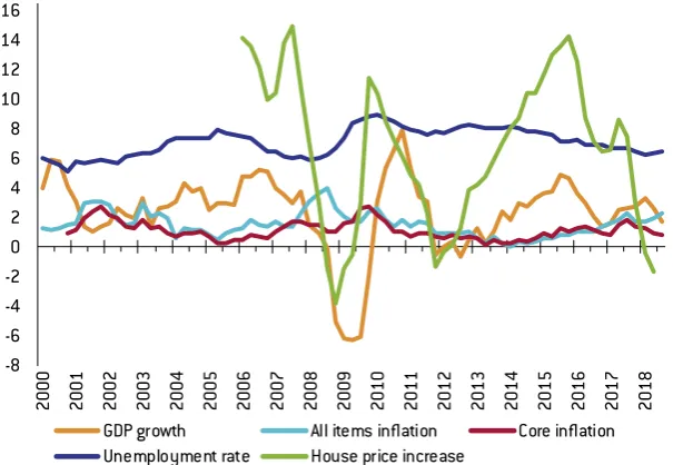
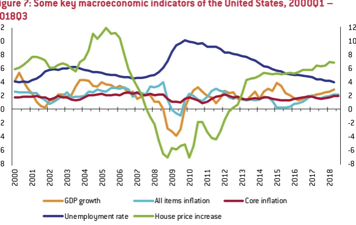
Figure 7: Some key macroeconomic indicators of the United States, 2000Q1 –
2018Q3
Source: Bruegel based on Federal Reserve Economic Data: Personal Consumption Expenditures: Chain-type Price Index (PCECTPI); Personal Con-sumption Expenditures: Chain-type Price Index Less Food and Energy (JCXFE); Real Gross Domestic Product (A191RO1Q156NBEA); Unemployment Rate, Aged 15-64, All Persons for the United States (LRUN64TTUSQ156S); All-Transactions House Price Index for the United States (USSTHPI). Note: percent change compared to the same quarter of the previous except for the unemployment, which is in percent of the labour force.
0 1 2 3 4 5 6 7 20 00 20 01 20 02 20 03 20 04 20 05 20 06 20 07 20 08 20 09 20 10 20 11 20 12 20 13 20 14 20 15 20 16 20 17 20 18 Federal funds effective rate 10-year government bond yield Longer-run federal funds rate projection by the FOMC (median) QE 1 QE 1 en
ds QE3
QE 2 QE 3 en ds QE 2 en ds ta pe rt an tru m -8 -6 -4 -2 0 2 4 6 8 10 12 -8 -6 -4 -2 0 2 4 6 8 10 12 20 00 20 01 20 02 20 03 20 04 20 05 20 06 20 07 20 08 20 09 20 10 20 11 20 12 20 13 20 14 20 15 20 16 20 17 20 18
GDP growth All items inflation Core inflation
[image:8.595.187.538.485.707.2]2.3 Bank of England: communication and forward guidance problems
unnecessarily pushed-up the 10-year yield
The Bank of England followed the footsteps of the Federal Reserve by linking interest rate increases to unemployment and later de-linking them. Communications misfortune was also followed by a significant increase in the long-term interest rate and a subsequent reversal.
On 4 July 2013, the Bank of England published a statement (an unusual move in the absence of a policy change) clarifying current policy and questioning whether expected future rates were in line with economic developments5. Then in August 2013, the Bank of England introduced
new forward guidance policies, linking increases in the interest rate to unemployment falling below 7 percent with three so-called ‘knock-out criteria’, including a quantitative threshold for inflation projections 18–24 months ahead (<2.5 percent) and anchored medium-term infla-tion expectainfla-tions and the absence of financial instability risks (Filandro and Hofmann, 2014; Whelan, 2018). The statement said: “the MPC intends not to raise Bank Rate from its current level of 0.5 percent at least until the Labour Force Survey headline measure of the unemployment rate
has fallen to a threshold of 7 percent, subject to the conditions below.”6
However, unemployment fell faster than foreseen by the Bank of England. Thus, in January and February 2014 the Bank of England updated its forward guidance, unlinking it from the decrease of the unemployment rate below 7 percent. Furthermore, in late June 2014, Mark Carney, the Governor of the Bank of England, suggested that the ‘new normal’ for the UK inter-est rate is 2.5 percent and the interinter-est rate could reach this value in early 20177.
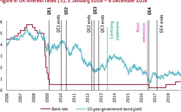
[image:9.595.183.537.435.654.2]These statements might have played a role in the strong increase in the 10-year UK govern-ment bond yield, from a value of about 2.2 percent in July 2013 to over 3 percent by September the same year. After that it fluctuated around 3 percent until July 2014, when it started to fall sig-nificantly, to as low as 1.4 percent by January 2015 (Figure 8). We cannot exclude the hypothesis that inappropriate forward guidance and its reversal contributed to a temporary upward shift of long-maturity interest rates, causing an unintended tightening of monetary conditions. Both headline and core inflation, however, remained well below 2 percent (Figure 9).
Figure 8: UK interest rates (%), 2 January 2006 – 6 December 2018
Source: Bank of England.
5 https://www.bankofengland.co.uk/-/media/boe/files/news/2013/july/mpc-july-2013.pdf.
6 Filandro and Hofmann (2014) found that futures rates did not drop following the formal introduction of forward guidance by the Bank of England in August 2013, suggesting that it was not effective in driving market expecta-tions, though the two-year futures rates did drop by more than 10 basis points in July 2013 when the MPC raised concerns about the appropriateness of market expectations for future policy rates.
7 https://www.bbc.com/news/business-28053045. 0
1 2 3 4 5 6
20
06
20
07
20
08
20
09
20
10
20
11
20
12
20
13
20
14
20
15
20
16
20
17
20
18
Bank rate 10-year government bond yield
Br
ex
it
re
fe
re
nd
um
QE
1
QE
3
QE
2
QE
4
QE
1
en
ds
QE
3
en
ds
QE
2
en
ds
Co
nf
us
in
g
st
at
em
en
ts
QE
4
en
Figure 9: Some key macroeconomic indicators of the United Kingdom, 2000Q1 – 2018Q3
Source: Eurostat. Note: percent change compared to the same quarter of the previous except for the unemployment, which is in percent of the labour force.
In terms of the actual exit from expansive policies in recent years, the UK experience has been quite similar to that of the US and Sweden: stopping net asset purchases hardly had an impact on long-term government yields, both after the third round of QE ended in November 2012 and the fourth (post-Brexit vote) round in March 2017. Even the actual 25 basis points interest rate increases by the Bank of England in November 2017 and August 2018 were not followed by any significant increase in long-term yields, similar to developments observed in the US after the first few interest rate hikes. However, in terms of more recent developments, the uncertain outlook around Brexit might also be playing a role in relation to market reactions.
Figure 10: ECB deposit facility interest rate and 10-year government bond yields of
four countries (%), 2 January 2000 – 7 December 2018
Source: Bruegel based on ECB and Bloomberg. Note: for asset purchases the announcement dates are indicated; the actual changes to purchased volumes took effect typically about 2 months later.
-16 -14 -12 -10 -8 -6 -4 -2 0 2 4 6 8 10 12 20 00 20 01 20 02 20 03 20 04 20 05 20 06 20 07 20 08 20 09 20 10 20 11 20 12 20 13 20 14 20 15 20 16 20 17 20 18
GDP growth All items inflation Core inflation
Unemployment rate House price increase
-1 0 1 2 3 4 5 6 7 8 20 00 20 01 20 02 20 03 20 04 20 05 20 06 20 07 20 08 20 09 20 10 20 11 20 12 20 13 20 14 20 15 20 16 20 17 20 18
France 10-year Germany 10-year Italy 10-year
Spain 10-year ECB deposit facility rate
"Whatever it takes" speech
[image:10.595.186.527.521.735.2]The conclusion that ending net asset purchases has a negligible impact on long-term gov-ernment bond yields seems to hold for the ECB too (so far): except for Italy, where domestic political shocks drove the interest rate up in recent months, in other larger euro-area countries, government bond yields have hardly changed since the ECB reduced and announced the end of net asset purchases (Figure 10).
3 A new normal in monetary policy?
Beyond the timing of monetary policy normalisation, the key questions are:
• To what level should the interest rate be increased?
• Should central bank balance sheets be reduced, and if so, to what level?
There are reasons to believe that interest rates will be lower and central bank balance sheets will be larger than they were in the pre-crisis period.
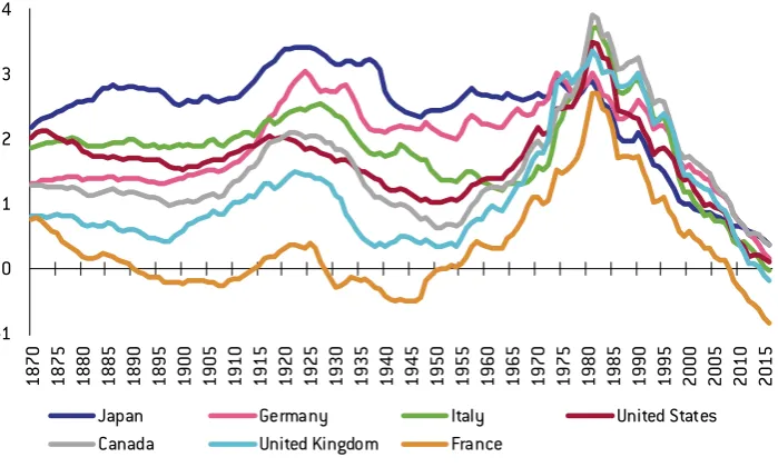
[image:11.595.185.535.515.725.2]Several papers have documented the secular decline in interest rates. A recent contribu-tion to this discussion was Del Negro et al (2018), who found that the trend in the world real interest rate for safe and liquid assets fluctuated close to 2 percent for more than a century, but has dropped close to zero over the past three decades. They find the same declining pattern in many advanced economies (Figure 11). These findings are consistent with the earlier estimates of Holston et al (2017) for four economies, Canada, the euro area, the United Kingdom and the United States. Typically, three main explanations are offered to explain this secular trend (Del Negro et al, 2018; Holston et al, 2017). First, the premium that international investors are willing to pay to hold safe and liquid assets has increased, partly because of the scarcity of safe assets in the context of a global savings glut. Second, lower productivity growth and consequently lower economic growth drive down the real interest rate. And third, demo-graphic factors also exert downward pressure on the natural rate of interest: populations are aging as people live longer, which encourages more saving, and birth rates have fallen, which reduces the rate of growth of the labour force and thus economic growth.
Figure 11: Estimated trend components in short-term real interest rates, 1870-2016
-1 0 1 2 3 4
18
70
18
75
18
80
18
85
18
90
18
95
19
00
19
05
19
10
19
15
19
20
19
25
19
30
19
35
19
40
19
45
19
50
19
55
19
60
19
65
19
70
19
75
19
80
19
85
19
90
19
95
20
00
20
05
20
10
20
15
Japan Germany Italy United States
Canada United Kingdom France
Williams (2018) argued that although there is uncertainty about the natural rate and its expected evolution, it is reasonable to assume that it will remain low, not far from current levels, in the foreseeable future. This would have major implications for monetary policy. A lower equilibrium interest rate implies that in recessions the (effective) zero lower bound would likely be reached more frequently, limiting the impact of traditional interest rate policy (Claeys and Demertzis, 2017; Foldén, 2018; Williams, 2018). Thereby, unconventional mon-etary policy measures would be used more regularly, leading to larger central bank balance sheets than what was observed before 2008.
We note that this otherwise sensible argument applies to a kind of long-term average cen-tral bank balance sheet size, but is not very helpful as a guide for current monetary exit strate-gies. The argument implies that in future monetary easing periods, balance sheet instruments will be used more often, but it does not imply that in a monetary policy normalisation phase, the balance sheet cannot return to its previous level if deemed appropriate.
Yet the first question to answer is whether the central bank balance sheet should be reduced at all. Foldén (2018) and Claeys and Demertzis (2017) discussed several arguments in favour of larger central bank balance sheets. This can improve the monetary transmission mechanism, because the large liquidity surplus (large reserves of banks held at the central bank8), can mitigate the risk of friction on the money market. Larger central bank balance
sheet can provide safe assets in the form of central bank liquidity. It can also reduce banks’ incentives for excessive maturity transformation, which would make banking less risky.
But there are a number of arguments against a large central bank balance sheet too. Central bank asset holdings could alter market pricing mechanism. Large asset holdings can limit further asset purchases in a next monetary easing phase if the supply of assets is limited. It might expose the central bank to financial risk9 and undue political influence, since large
holding of government and/or private sector assets could risk politicians wishing to rely on central bank asset purchases for certain political goals10.
It is notable that the Federal Reserve remained ambiguous about the targeted size of balance sheet reduction. Its communications related to monetary policy normalisation11
have not specified what amount of holdings are needed to implement monetary policy: “The Committee intends that the Federal Reserve will, in the longer run, hold no more securities than necessary to implement monetary policy efficiently and effectively, and that it will hold primarily Treasury securities, thereby minimizing the effect of Federal Reserve holdings on the
allocation of credit across sectors of the economy”12.
Moreover, the monetary policy normalisation communication states: “Gradually reducing the Federal Reserve’s securities holdings will result in a declining supply of reserve balances. The Committee currently anticipates reducing the quantity of reserve balances, over time, to a level appreciably below that seen in recent years but larger than before the financial crisis; the level will reflect the banking system’s demand for reserve balances and the Committee’s decisions
about how to implement monetary policy most efficiently and effectively in the future.” Since
the increase in bank reserves since 2008 was primarily the reflection of asset purchases, a bank reserve stock larger than before the financial crisis would also imply a larger stock of asset holdings.
For these reasons, we conclude that the Federal Reserve remained ambiguous about the targeted size of its balance sheet reduction. The likely reason for this ambiguity is the lack of experience with balance sheet reductions. Most likely, the future direction of balance sheet reduction will result from a learning process, whereby the currently announced pace of
8 See Darvas and Pichler (2018) for an analysis of bank reserve holdings in the euro area. 9 See Chiacchio et al (2018) for an assessment of the importance of central bank profits.
10 The size of the central bank balance sheet also depends on the way monetary policy is conducted, on the exchange rate regime, past monetary policy actions, central bank tasks, profits distribution. Thereby there is no universal benchmark for ‘normal’ central bank balance sheets.
11 https://www.federalreserve.gov/monetarypolicy/policy-normalization.htm.
balance sheet reduction will continue until the objectives of the Federal Reserve (2 percent inflation and full employment) are achieved in a sustainable manner, while changes to the pace should be expected if the objectives will be at risk.
Such inexperience also characterises the euro area, which calls for a similarly cautious approach from the ECB in its balance sheet reduction efforts. The advice one can make about the normalisation of central bank balance sheet policies is that the strategy should start only after the macroeconomic goals of the central bank has been achieved. The balance sheet size reduction should be gradual to minimise disruptions to the functioning of financial markets and conditional on not jeopardising the macroeconomic goals.
4 Monetary policy exit in the euro area when
the inflation outlook is uncertain
The primary objective of the ECB is price stability, which was defined by the ECB Governing Council in 1998 as inflation below two percent13. Given that Eurostat publishes inflation data
rounded to one digit after the decimal, inflation rates in the range from 0.1 percent to 1.9 per-cent correspond to the definition of price stability. However, in 2003 the Governing Council clarified that “in the pursuit of price stability it aims to maintain inflation rates below, but close
to, 2% over the medium term”14. The duration of medium term has not been defined by the
ECB, but is typically understood as a period of about 18 month or slightly longer15. This
some-what ambiguous clarification has been extensively used in ECB communication since 2003. While the ECB does not have a formal inflation target, the clarification is widely understood as a target rate of inflation below but close to two percent.
4.1 The ECB forecasting failures
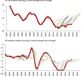
Euro-area headline inflation long undershot this 2 percent threshold in 2013-17, but it reached the range of 2.0-2.2 percent between June-November 2018 (compared to the same month of the previous year). The recent increase in headline inflation is partly due to oil price increase, while core inflation (which excludes items with volatile prices like food and energy) remains close to 1 percent. The September 2018 forecast of the ECB itself expects the headline inflation to fall back to 1.5 percent by the third quarter of 2019, after which a speeding up is foreseen to 1.8 percent by the end of 2020. The acceleration of core inflation to 1.5 percent on average in 2019 and 1.8 percent on average in 2020 is also predicted by the ECB.
The predicted core inflation increase partly reflects the economic recovery of the euro area and labour market improvements. Yet the large and systemic forecast errors made by the ECB16 raises serious doubts about the reliability of the current ECB forecasts. Panel A of Figure
12 shows that the ECB has systematically overestimated the future developments of core inflation (at least since December 2013, the first time when core inflation forecasts were made
13 https://www.ecb.europa.eu/mopo/strategy/pricestab/html/index.en.html. 14 Ibid.
15 The ECB’s webpage on ‘Medium-term orientation’ states: “It is impossible for any central bank to keep inflation always at a specific point target or to bring it back to a desired level within a very short period of time. Consequently, monetary policy needs to act in a forward-looking manner and can only maintain price stability over longer periods of time. At the same time, to retain some flexibility, it is not advisable to specify ex-ante a precise horizon for the conduct of monetary policy, since the transmission mechanism spans a variable, uncertain period of time. Also, the optimal monetary policy response to ensure price stability always depends on the specific nature and size of the shocks affecting the economy.” See: https://www.ecb.europa.eu/mopo/strategy/princ/html/orientation.en.html.
public) and the forecasts errors were rather significant. Similar conclusion applies to headline inflation, which was systematically over-predicted in 2014-16 (panel B). Since 2017, actual inflation has increased along with the forecast, but this was the outcome of two incorrect views: the forecast increase in core inflation (which has not happened) and the assumption of broadly unchanged energy prices (which have increased rapidly).
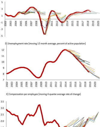
It is notable that while the ECB has over-predicted inflation developments, it has under-predicted GDP growth since 2014. That is, actual GDP growth has turned out to be systematically higher than ECB forecasts (panel C). This also implies that the underlying assumed relationship between growth and inflation was even more inaccurate: better than expected GDP growth should have resulted in higher than expected core and headline infla-tion, but in fact, core inflation (and also headline inflation for a number of years) has been significantly lower than expected.
Labour market forecasts are similarly characterised by large and systematic errors. The forecast errors of the unemployment rate (panel D) mirror the forecast errors of GDP: as GDP growth became better than expected, the unemployment rate also fell faster than expected, which are consistent developments. But the unemployment rate forecast errors highlight that the ECB’s underlying Phillips curve assumption is flawed: faster than expected unemploy-ment rate decline should have led to faster than expected rising inflation, but on the contrary, core inflation (and also headline inflation until 2016) turned out to be lower than predicted.
[image:14.595.182.528.409.766.2]Wage forecasts also turned out to be grossly inadequate in 2013-16, though since 2017 wages have generally grown in line with predictions (panel E). Yet this particular recent wage growth forecast success is inconsistent with the faster than expected reduction in the unem-ployment rate and the lower than expected core inflation increase, highlighting the uncer-tainty of the underlying economic relationships assumed in ECB forecasting exercises.
Figure 12: ECB staff macroeconomic projections for the euro area, average annual values
0.5 1 1.5 2 2.5 20 02 20 03 20 04 20 05 20 06 20 07 20 08 20 09 20 10 20 11 20 12 20 13 20 14 20 15 20 16 20 17 20 18 20 19 20 20 -0.5 0 0.5 1 1.5 2 2.5 3 3.5 4 20 02 20 03 20 04 20 05 20 06 20 07 20 08 20 09 20 10 20 11 20 12 20 13 20 14 20 15 20 16 20 17 20 18 20 19 20 20
B) Headline inflation (moving 12-month average rate of change) A) Core inflation (moving 12-month average rate of change)
-5 -3 -1 1 3 5 20 02 20 03 20 04 20 05 20 06 20 07 20 08 20 09 20 10 20 11 20 12 20 13 20 14 20 15 20 16 20 17 20 18 20 19 20 20 7 8 9 10 11 12 20 02 20 03 20 04 20 05 20 06 20 07 20 08 20 09 20 10 20 11 20 12 20 13 20 14 20 15 20 16 20 17 20 18 20 19 20 20
Source: Bruegel based on Eurostat and various vintages of ECB forecasts. Note: Actual data is the thick red line (moving 12-month or 4-quar-ter averages), while the thin colourful lines show the ECB forecasts made in each quar4-quar-ter. ECB forecasts are available for annual values. That’s why we use the 12-month (or 4-quarter) average rate of change for the actual data in the case of inflation, GDP growth and the wage growth, while the 4-quarter moving average rate of unemployment. Such moving average data is (practically) equal the annual average in the 4th quarter (in case of quarterly data) or December (in case of monthly data) of each year. In the chart the end observation (in Q4 or
December of various years) of each forecast curve corresponds to the annual average forecast numbers published by the ECB. We have linearly interpolated the annual average forecast data and the data in the quarter (or month) of the date of the forecast. Note that the actual data for the quarter (or month) when the forecast is made is not yet known at the time of the forecast, given data publication delays.
Certainly, the ECB is not the only institution whose forecasts turned out to be incorrect. Many other central banks, international institutions and other forecasters made large casting errors even in the last five years, when economic conditions improved. Such fore-casting failures should foster a general debate on forefore-casting practices. Yet the ECB’s forecast errors and its inability to lift core inflation above 1 percent have major implications.
1.0 1.5 2.0 2.5 3.0 3.5 20 02 20 03 20 04 20 05 20 06 20 07 20 08 20 09 20 10 20 11 20 12 20 13 20 14 20 15 20 16 20 17 20 18 20 19 20 20
E) Compensation per employee (moving 4-quarter average rate of change) public) and the forecasts errors were rather significant. Similar conclusion applies to headline
inflation, which was systematically over-predicted in 2014-16 (panel B). Since 2017, actual inflation has increased along with the forecast, but this was the outcome of two incorrect views: the forecast increase in core inflation (which has not happened) and the assumption of broadly unchanged energy prices (which have increased rapidly).
It is notable that while the ECB has over-predicted inflation developments, it has under-predicted GDP growth since 2014. That is, actual GDP growth has turned out to be systematically higher than ECB forecasts (panel C). This also implies that the underlying assumed relationship between growth and inflation was even more inaccurate: better than expected GDP growth should have resulted in higher than expected core and headline infla-tion, but in fact, core inflation (and also headline inflation for a number of years) has been significantly lower than expected.
Labour market forecasts are similarly characterised by large and systematic errors. The forecast errors of the unemployment rate (panel D) mirror the forecast errors of GDP: as GDP growth became better than expected, the unemployment rate also fell faster than expected, which are consistent developments. But the unemployment rate forecast errors highlight that the ECB’s underlying Phillips curve assumption is flawed: faster than expected unemploy-ment rate decline should have led to faster than expected rising inflation, but on the contrary, core inflation (and also headline inflation until 2016) turned out to be lower than predicted.
[image:15.595.181.516.72.497.2]Wage forecasts also turned out to be grossly inadequate in 2013-16, though since 2017 wages have generally grown in line with predictions (panel E). Yet this particular recent wage growth forecast success is inconsistent with the faster than expected reduction in the unem-ployment rate and the lower than expected core inflation increase, highlighting the uncer-tainty of the underlying economic relationships assumed in ECB forecasting exercises.
Figure 12: ECB staff macroeconomic projections for the euro area, average annual values
0.5 1 1.5 2 2.5 20 02 20 03 20 04 20 05 20 06 20 07 20 08 20 09 20 10 20 11 20 12 20 13 20 14 20 15 20 16 20 17 20 18 20 19 20 20 -0.5 0 0.5 1 1.5 2 2.5 3 3.5 4 20 02 20 03 20 04 20 05 20 06 20 07 20 08 20 09 20 10 20 11 20 12 20 13 20 14 20 15 20 16 20 17 20 18 20 19 20 20
B) Headline inflation (moving 12-month average rate of change) A) Core inflation (moving 12-month average rate of change)
-5 -3 -1 1 3 5 20 02 20 03 20 04 20 05 20 06 20 07 20 08 20 09 20 10 20 11 20 12 20 13 20 14 20 15 20 16 20 17 20 18 20 19 20 20 7 8 9 10 11 12 20 02 20 03 20 04 20 05 20 06 20 07 20 08 20 09 20 10 20 11 20 12 20 13 20 14 20 15 20 16 20 17 20 18 20 19 20 20
4.2 Can certain labour market factors explain the forecasting failures?
The labour supply in the euro area has increased for two main reasons:
• The labour force participation rate has been steadily increasing (Figure 13);
• Net immigration into the euro area was also substantial, and not just because of the major inflows of refugees in 2015-16.
[image:16.595.184.519.280.450.2]An expanding labour force could put wages under downward pressure. If the ECB has persistently underestimated the expansion of the labour force, this factor could explain the persistent forecast errors in relation to wage and price increases. But such a persistent under-estimation of labour force expansion is not consistent with the unemployment rate forecast errors, because faster than expected labour force growth should have resulted in larger than expected unemployment. But the opposite has happened.
Figure 13: Labour force participation rate (age 15-64, % of population),
1997Q1-2018Q2
65 70 75 80 85
19
97
19
98
19
99
20
00
20
01
20
02
20
03
20
04
20
05
20
06
20
07
20
08
20
09
20
10
20
11
20
12
20
13
20
14
20
15
20
16
20
17
20
18
Sweden
Japan
United Kingdom
United States
Euro area
Source: Bruegel; updated from Darvas and Pichler (2017) using Eurostat’s ‘Employment and activity by sex and age - quarterly data [lfsi_emp_q]’ dataset.
Another explanation for the repeated forecast errors could be related to the esti-mate of the non-accelerating wage rate of unemployment (NAWRU). NAWRU cannot be observed, but is estimated using certain econometric techniques17. Taken literally without
the consideration of any additional factor, the NAWRU concept suggests that when actual unemployment is the same as the NAWRU, wage growth does not accelerate. But if actual unemployment is below the NAWRU, wage growth acceleration should be expected, while an unemployment rate above the NAWRU should lead to a deceleration of wage growth. A possible explanation for the ECB forecast errors could be that in real-time the ECB thought that the actual unemployment rate was already below the NAWRU and thus predicted an increase in wage growth and inflation. But a year later it could have turned out that the ini-tial NAWRU estimate was wrong and the new NAWRU estimate is much lower, and therefore there was excessive labour supply in the past year which kept wage growth and inflation growth low, while unemployment fell to approach the NAWRU. Persistent NAWRU estima-tion errors could explain the persistent forecast errors.
Unfortunately, the ECB does not publish its NAWRU estimates. However, the European Commission publishes its NAWRU estimates, which are made using the commonly agreed methodology in the EU. While Havik et al (2014, p11) define the concept as “trend un/
employment to be consistent with stable, nonaccelerating, (wage) inflation (NAWRU)”, in practice either the change in the growth rate of nominal unit labour costs (related to the so-called ‘traditional Keynesian Phillips curve’ – TKP) or the growth rate of nominal unit labour cost (related to the so-called ‘new Keynesian Phillips curve’ – NKP) is analysed18.
Some additional variables also enter the equations used to estimate the NAWRU, namely labour productivity growth and a terms-of-trade indicator in the TKP framework, and lags in the NKP framework. Thereby, a European Commission NAWRU estimate cannot be taken literally to indicate the non-accelerating wage rate of unemployment, partly because unit labour cost is studied (and thus instead of the name NAWRU, the name ‘non-accelerating unit labour cost rate of unemployment’ should be used), and partly because of the other factors considered. Still, the gap between the actual unemployment rate and the Commis-sion’s NAWRU estimate could be a proxy for the labour market pressure on nominal wage growth developments.
The ECB’s own estimates might not be much different from the Commission estimates, so we look at Commission’s NAWRU estimates (Figure 14). The euro-area NAWRU estimates were revised downward for two main reasons. First, unit labour costs and wage growth have not picked up. Second, the estimated model assumes smooth development of the NAWRU, so an actual fall in the unemployment rate leads to downward revisions of past NAWRU estimates.
[image:17.595.183.517.396.625.2]However, Figure 14, which shows the actual unemployment rate data available in autumn 2018 and the real-time NAWRU estimates, highlights that the actual rate has been persistently higher than the real-time NAWRU estimates.
Figure 14: Actual unemployment rate and the European Commission’s NAWRU
estimates
Source: Bruegel based on various vintages of the AMECO database related to the European Commission’s forecasts, see https://ec.europa. eu/info/business-economy-euro/economic-performance-and-forecasts/economic-forecasts_en.
Table 1 reports the perceived real-time gap between the unemployment rate and the NAWRU estimate, because, for example, in autumn 2013 the actual unemployment rate for 2013 was not yet known and an estimate was made.
18 Havik et al (2014) reports that the EU’s Economic Policy Committee endorsed a NKP specification for 21 of the 28 EU member states (of which 12 are currently members of the euro area) and a TKP specification for the remaining 7 countries (all 7 are members of the euro area).
7 8 9 10 11 12
19
98
20
00
20
02
20
04
20
06
20
08
20
10
20
12
20
14
20
16
20
18
Actual unemployment rate
2013 autumn NAWRU estimate
2014 autumn NAWRU estimate
2015 autumn NAWRU estimate
2016 autumn NAWRU estimate
2017 autumn NAWRU estimate
Table 1: Estimated real-time gap between the actual unemployment rate and the
NAWRU (European Commission estimates)
real time estimate 2018 autumn estimate
2013 spring 1.3 2.6
2013 autumn 1.4 2.6
2014 spring 1.7 2.4
2014 autumn 1.7 2.4
2015 spring 1.2 2
2015 autumn 1.1 2
2016 spring 0.7 1.3
2016 autumn 1 1.3
2017 spring 0.5 0.7
2017 autumn 0.5 0.7
2018 spring 0.1 0.3
2018 autumn 0.3 0.3
Source: Bruegel based on various vintages of the European Commission forecast, https://ec.europa.eu/info/business-economy-euro/eco-nomic-performance-and-forecasts/economic-forecasts_en.
Table 1 shows that there has always been a positive gap between the unemployment rate and the NAWRU in the European Commission’s real-time estimates. This should have implied an expected deceleration in the nominal unit labour costs growth rate, and possi-bly nominal wages too and therefore the ECB should have not predicted wage growth (and consequent inflation) acceleration in the first place. Because of the later downward revisions of the NAWRU estimates, the gaps between the actual unemployment rate and NAWRU were apparently greater in autumn 2018 than in real time, but the important point that there was a positive gap even in real-time estimates.
Inflation forecasts takes into account other factors beyond the NAWRU. Nevertheless, it is interesting to note that while the perceived unemployment gap has narrowed (Table 1) and thus its deflationary impact has also narrowed, the predicted pace of wage growth and core inflation acceleration were rather similar during the past five years (Figure 12). This might indicate that NAWRU was not an important aspect of the ECB’s core inflation forecasts.
Looking ahead, if the expansion of the labour force slows down and the recently acceler-ated wage growth continues, we might perhaps see the rise of core inflation. Furthermore, if the NAWRU concept is valid after all and current estimates are somehow more reliable than the unreliable past estimates, then the elimination of the positive gap between the actual unemployment rate and the estimated NAWRU (Table 1) might also suggest that wage pres-sure could increase in the coming years.
But a number of factors call for caution about the potential for increased euro-area core inflation:
• In the euro area, the trend of labour-force participation growth continues; higher la-bour-force participation rates in Japan, Sweden and the United Kingdom suggest that there is still ample room for the euro-area rate to further increase (Figure 12); • Core inflation has so far remained stable despite some wage increases (Figure 12); • Current wage increases still remain short of the wage growth observed in the early 2000s
when core inflation was close to 2 percent;
in the early 2000s. Those part-time workers who wish to work full time could exert down-ward pressure on wage growth;
• The Phillips curve, which in its most basic setup measures the relationship between unemployment and wage growth, is found to become flatter in advanced countries (Ku-ttner and Robinson, 2010; Claeys et al, 2018). This implies that the relationship between demand conditions (including unemployment/underemployment) and wage and price inflation is weaker and thus a further fall in unemployment (or underemployment) is less likely to be followed by increased inflation.
These are mainly pertinent over the medium and long terms, but there are also some shorter term-issues that call for caution about the possibility of core inflation acceleration. Euro-area business surveys show some darkening of the economic outlook, which might have already contributed to the slowdown in economic growth in the third quarter of 2018. The recent rapid fall in oil prices will soon exert downward pressure on headline inflation and might also hold back core inflation.
All these factors suggest a high level of caution when considering when the ECB might raise interest rates and the path of the prospective increase, if the ECB continues to pursue a goal of close to two percent inflation.
4.3 What is needed? More time, more monetary stimulus or a new inflation
target?
Market-based inflation expectations already show concern about the credibility of the ECB’s somewhat ambiguous ‘below, but close to, two percent over the medium term’ clarification of its inflation goal. Even though headline inflation was in the range of 2.0-2.2 percent from June to November 2018 and wage growth has recently accelerated, market-based expectations of average headline inflation in the next five years had fallen to 1.2 percent by early December 2018 (Panel A of Figure 15)19. Longer-term expectations
also fell (Panel B of Figure 15): the so-called 5y5y market-based inflation expectation (five year average inflation expected in five years’ time) fell from values of between 2-2.5 per-cent in 2004-14 to 1.6 perper-cent in December 2018. While 1.6 perper-cent might as arguably be considered still relatively close to two percent, the 1.2 percent expected average inflation in the next five years is not so close and further repeated forecasting failures might lead to further falls in expected inflation, ultimately undermining the ECB’s credibility.
The Bank of Japan is a telling example. There seems to be sufficient evidence to con-clude that the Bank of Japan has failed to reach the 2 percent inflation target though it has an even more forceful monetary policy toolkit than that applied by the ECB (Shirai, 2018). And it is unlikely that the target will be reached in the years to come. Long-term headline inflation expectations have fallen back to zero (panel B of Figure 15). In our view, the Bank of Japan will probably have to acknowledge its failure to reach the 2 percent target and then revise the target.
At the same time the Federal Reserve was successful in bringing inflation back to two percent. Whether the structural characteristics of the euro area are closer to Japan or to the US is an important question for discussion. However, the ECB’s failure to raise core inflation above one percent with a large monetary policy arsenal at a time when GDP growth and employment turned out to be better than expected should provoke a discus-sion about the forecasting failures and the ability of the ECB to influence core inflation.
More time is needed to see if the forecasting failures of the past five years were driven by factors whose impact will gradually fade away, or if the ECB’s ability to lift core infla-tion has been compromised. In the meantime, the ECB will surely stick to its current aim of below, but close to, 2 percent inflation over the medium term. For this period we recommend an extremely cautious approach to monetary tightening. The forecasts
selves should not be enough to justify a rate increase. A rate increase is only recommended after a significant increase in actual core inflation. We also suggest making this intention clear in the ECB’s forward guidance. In our view, the ECB’s current forward guidance is insufficient:
“The Governing Council expects the key ECB interest rates to remain at their present levels at
least through the summer of 2019, and in any case for as long as necessary to ensure the contin-ued sustained convergence of inflation to levels that are below, but close to, 2 percent over the
medium term.” (13 September 2018 ECB press release20). Likewise, we recommend the size
[image:20.595.183.525.240.666.2]of the ECB’s balance sheet should be kept unchanged in the foreseeable future, and a gradual process of its reduction should begin only after the first few interest rate hikes, conditional on not jeopardising the inflation outlook.
Figure 15: Market-based five year average headline inflation expectations, June
2004 – December 2018
Source: Bruegel based on Bloomberg; monthly average data is reported. Note: December 2018 values are based on the first five days of the month.
20 https://www.ecb.europa.eu/press/pr/date/2018/html/ecb.mp180913.en.html. -3
-2 -1 0 1 2 3 4 5
20
04
20
05
20
06
20
07
20
08
20
09
20
10
20
11
20
12
20
13
20
14
20
15
20
16
20
17
20
18
UK
United States
Euro area
Japan A) Next five years
B) Five years starting in five years’ time
-2 -1 0 1 2 3 4 5
20
04
20
05
20
06
20
07
20
08
20
09
20
10
20
11
20
12
20
13
20
14
20
15
20
16
20
17
20
18
UK
United States
Euro area
Such a cautious monetary policy exit strategy might work, but we cannot exclude the pos-sibility of repeated failures in forecasting and in lifting core inflation. Such an outcome would undermine the credibility of the ECB and would necessitate a discussion on either the deploy-ment of new tools to influence core inflation, or a possible revision of the ECB’s inflation goal.
5 Euro-area countries face different
financial stability risks
Beyond the overall macroeconomic issues, central banks might weigh the issue of financial stability when considering the normalisation of monetary policy. Financial stability concerns are on the rise in some euro-area countries. As argued by Darvas and Merler (2013), there are strong interactions between monetary policy and financial stability policy: both have implications for the other. That’s why there should be close cooperation (and not a Chinese wall) between these two main policy areas, though they should operate with different instruments to achieve their different goals.
Monetary policy should not be used to achieve a financial stability objective, partly because the main monetary policy instrument, the interest rate, is too broad and ultimately quite inef-fective in dealing with the build-up of financial imbalances (Claeys and Darvas, 2015; Claeys
et al, 2018). For example, Posen (2009) showed that it is difficult to find a clear relationship
between interest-rate tightening and the growth rate of asset prices. He concluded that the use of interest rates to prevent the build-up of financial imbalances appears to be ineffective. In rela-tion to the housing bubble in the United Kingdom before the crisis, Bean et al (2010) estimated that additional increases in the Bank of England’s main rate by several percentage points would have been needed to stabilise house prices. Such interest rate increases would have reduced inflation to levels significantly below the Bank of England’s 2 percent target, and would have had significant negative effects on output. The Swedish example (section 2.1) also highlighted that the 2010-11 monetary policy tightening for financial stability reasons backfired and necessitated an even more significant monetary easing later in response to weaker inflation, growth and employment. Moreover, the Swedish household debt-to-income ratio was not affected by the 2010-11 policy of tightening.
Furthermore, monetary tightening for reasons of financial instability might have other unin-tended effects, especially in open economies. An increase in capital inflows because of higher interest rates can partially offset the dampening effect of higher rates on credit. A monetary tightening can also cause a migration of activity from the regulated banking sector to the shad-ow-banking sector (Nelson et al, 2015).
Therefore, even though close cooperation is recommended between financial stability and monetary policymaking, we advise against using monetary policy tools for financial stability purposes.
The area situation is further complicated by the significant differences between euro-area members, as argued by Darvas and Pichler (2018). Financial stability concerns would suggest an interest rate increase in some countries (eg Slovakia, where household loans and house prices are increasing very rapidly), but not in others (eg Italy, where household loans are stagnant and house prices continue to fall). But monetary policy cannot discriminate between euro-area countries, so beyond the conceptual issues, the euro area’s variability further high-lights that monetary policy is not a useful instrument for containing financial stability risks.
Table 2: Macroprudential policy measures in European countries, mid-2018
Systemic r
isk b
uffers
(S
yRB)
Co
un
ter
cy
clic
al c
apital
b
uffers (CC
yB)
Other measur
es aime
d
at r
eal esta
te m
ar
ket
G
lobal systemic
ally
im
p
or
tan
t institutions
(G-SII
s)
Other measur
es not
fundamen
tally r
ela
te
d
to r
eal esta
te
Wh
at other measur
es
not tar
getin
g the r
eal
esta
te m
ar
ket
Austria Y Y
Belgium Y Y
Capital add-on for banks with excessive
trading activities as measured according
to two indicators (volume-based,
risk-based).
Bulgaria Y Y Y
stress-tests, capital rules for bank dividend distribution,
reporting rules, exposure to Greek
equity, liquidity coverage ratio
Cyprus Y Y
stress-tests, caps on deposit interest rates,
liquidity coverage requirement add-on Czech
Republic Y Y Y
Denmark Y Y Y Y
limits to lending growth, short funding
and large exposures
Estonia Y Y
Finland Y Y Y
France Y Y Y
French Systemically Important Institutions
shall not incur an exposure that exceeds
5 % of their eligible capital for NFCs or group of connected NFCs assessed to be
highly indebted.
Croatia Y Y
Hungary Y Y Y
liquidity coverage ratios, foreign exchange assets rules
Ireland Y Y Y
Introduction of a set of requirements for loan originating alternative investment
funds.
Iceland Y Y Y
Liechtenstein Y Y
Luxembourg Y Y stress-tests
Latvia Y
Malta Y Y NPL limits
Netherlands Y Y Y
Norway Y Y Y Y liquidity coverage
ratios
Poland Y Y Y liquidity coverage ratios
Portugal Y
Romania Y Y Y
consumer loan rules, foreign exchange
assets rules
Sweden Y Y Y Y Y
Pillar II capital add-on, increased
transparency in capital requirements,
increased risk weights for corporate
exposures, risk weights
Slovenia Y Y
cap on deposit interest rates,
loan-to-deposit ratios
Slovakia Y Y Y Y maturity limits for consumer loans
United
Kingdom Y Y Y Y leverage ratios
Germany Y
Spain Y
Italy Y