Post-common envelope binaries from SDSS - XV. Accurate stellar parameters for a cool 0.4 M⊙ white dwarf and a 0.16 M⊙ M dwarf in a 3 h eclipsing binary

(1)

Post-common envelope binaries from SDSS – XV. Accurate stellar

parameters for a cool 0.4 M

white dwarf and a 0.16 M

M dwarf

in a 3 h eclipsing binary

S. Pyrzas,

1

B. T. G¨ansicke,

1

S. Brady,

2

S. G. Parsons,

1

T. R. Marsh,

1

D. Koester,

3

E. Breedt,

1

C. M. Copperwheat,

1

A. Nebot G´omez-Mor´an,

4

A. Rebassa-Mansergas,

5

M. R. Schreiber

5

and M. Zorotovic

5

1_{Department of Physics, University of Warwick, Coventry CV4 7AL} 2_{AAVSO, 5 Melba Drive, Hudson, NH 03051, USA}

3_{Institut f¨ur Theoretische Physik und Astrophysik, University of Kiel, 24098 Kiel, Germany}

4_{Universit´e de Strasbourg, CNRS, UMR7550, Observatoire Astronomique de Strasbourg, 11 Rue de l’Universit´e, F-67000 Strasbourg, France} 5_{Departamento de F´ısica y Astronom´ıa, Facultad de Ciencias, Universidad de Valpara´ıso, Avenida Gran Bretana 1111, Valpara´ıso, Chile}

Accepted 2011 August 31. Received 2011 August 26; in original form 2011 July 27

A B S T R A C T

We identify SDSS J121010.1+334722.9 as an eclipsing post-common-envelope binary, with an orbital period of Porb = 2.988 h, containing a very cool, low-mass, DAZ white dwarf and a low-mass main-sequence star of spectral type M5. A model atmosphere analysis of the metal absorption lines detected in the blue part of the optical spectrum, along with the

Galaxy Evolution Explorernear-ultraviolet flux, yields a white dwarf temperature ofTeff,WD= 6000±200 K and a metallicity value of log [Z/H]= −2.0±0.3. The NaIλλ8183.27, 8194.81 absorption doublet is used to measure the radial velocity of the secondary star,Ksec =251.7± 2.0 km s−1, and FeIabsorption lines in the blue part of the spectrum provide the radial velocity of the white dwarf,KWD =95.3±2.1 km s−1, yielding a mass ratio ofq=0.379±0.009. Light-curve model fitting, using the Markov chain Monte Carlo method, gives the inclination angle asi=(79◦.05–79.◦36)±0◦.15, and the stellar masses asMWD =0.415±0.010 M andMsec = 0.158±0.006 M. Systematic uncertainties in the absolute calibration of the photometric data influence the determination of the stellar radii. The radius of the white dwarf is found to beRWD =(0.0157–0.0161)±0.0003 Rand the volume-averaged radius of the tidally distorted secondary isRsec,vol.aver. =(0.197–0.203)±0.003 R. The white dwarf in SDSS J121010.1+334722.9 is a very strong He-core candidate.

Key words: binaries: close – binaries: eclipsing – stars: fundamental parameters – stars: individual: SDSS 121010.1+334722.9 – stars: late-type – white dwarfs.

1 I N T R O D U C T I O N

Our understanding of stellar structure and evolution leads to the fun-damental prediction that the masses and radii of stars obey certain mass–radius (M–R) relations. The calibration and testing of theM–R relations require accurate and model-independent measurements of stellar masses and radii, commonly achieved with eclipsing binaries (e.g. Andersen 1991; Southworth & Clausen 2007).

Among main-sequence (MS) stars, M dwarfs of low mass (<0.3 M) are the most ubiquitous. However, few eclipsing low-mass MS+MS binaries are known (e.g. L´opez-Morales 2007;

_{E-mail: [email protected]}

Morales et al. 2009; C¸ akırlı & Ibano˘glu 2010; Dimitrov & Kjurkchieva 2010; Irwin et al. 2010 and references therein) and have accurate measurements of their masses and radii, affecting the calibration of the low-mass end of the MSM–Rrelation. To fur-ther complicate matters, existing measurements consistently result in radii up to 15 per cent larger and effective temperatures 400 K or more below the values predicted by theory (e.g. Ribas 2006; L´opez-Morales 2007). This is not only the case for low-mass MS+MS binaries (Bayless & Orosz 2006), but it is also present in field stars (Berger et al. 2006; Morales, Ribas & Jordi 2008) and the host stars of transiting extrasolar planets (Torres 2007).

The situation is similar for white dwarfs (WDs), the most com-mon type of stellar remnant. Very few WDs have model-independent measurements of their masses and radii (see Parsons et al. 2010a),

2011 The Authors

at The University of Sheffield Library on November 28, 2016

http://mnras.oxfordjournals.org/

(2)

and eclipsing WD+WD binaries have only recently been discov-ered (Steinfadt et al. 2010; Brown et al. 2011; Parsons et al. 2011). Consequently, the finite temperature M–R relation of WDs (e.g. Wood 1995; Panei, Althaus & Benvenuto 2000) remains largely untested by observations (Provencal et al. 1998).

An alternative approach leading to accurate mass and radius mea-surements for WDs and MS stars is the study of eclipsing WD+MS binaries. Until recently, the population of eclipsing WD+MS bi-naries had stagnated with only seven systems known (see Pyrzas et al. 2009, for a list), a direct result of the small number of the en-tire WD+MS binaries sample (∼30 systems; Schreiber & G¨ansicke 2003).

However, in recent years, progress has been made thanks to the Sloan Digital Sky Survey (SDSS; York et al. 2000). A dedicated search for WD+MS binaries contained in the spectroscopic SDSS Data Release 6 (DR6; Adelman-McCarthy et al. 2008) and Data Re-lease 7 (DR7; Abazajian et al. 2009) yielded more than 1600 systems (e.g. Rebassa-Mansergas et al. 2010), of which ∼1/3 are (short-period) post-common-envelope binaries (PCEBs; Schreiber et al. 2008). The majority of these PCEBs contain low-mass, late-type M dwarfs (Rebassa-Mansergas et al. 2010), while a large percentage of the WD primaries are of low mass as well (Rebassa-Mansergas et al. 2011).

A significant fraction of eclipsing systems should exist among this sample of PCEBs. Identifying and studying these eclipsing systems will substantially increase the observational constraints on theM–Rrelation of both WDs and MS stars. Therefore, we have begun the first dedicated search for eclipsing WD+MS binaries in the SDSS, and five new systems have already been published (Nebot G´omez-Mor´an et al. 2009; Pyrzas et al. 2009, but see also Drake et al. 2010 for a complementary sample).

SDSS J121010.1+334722.9 (henceforth SDSS 1210), the subject of this paper, is one of the new systems identified in this search. In what follows, we present our observations (Section 2), deter-mine the orbital period and ephemeris (Section 3) and analyse the spectrum of the WD (Section 4). Radial velocity measurements (Section 5) combined with light-curve fitting (Section 6) lead to the determination of the masses and radii of the binary components (Section 7). We also explore the past and future evolution of the system (Section 8).

2 TA R G E T I N F O R M AT I O N , O B S E RVAT I O N S A N D R E D U C T I O N S

SDSS 1210 was discovered by Rebassa-Mansergas et al. (2010) as a WDMS binary dominated by the flux of a low-mass companion with a spectral type M5V, suggesting that the WD must be very cool. Inspecting the NaIλλ8183.27, 8194.81 doublet in the six SDSS subspectra1_{with exposure times of 15–30 min taken over the}

course of three nights, we found large radial velocity variations that strongly suggested an orbital period of a few hours. We obtained time-series photometry of SDSS 1210 with a 16-inch telescope equipped with an ST8-XME CCD camera, with the aim to measure the orbital period from the expected ellipsoidal modulation, and immediately detected a shallow eclipse in the light curve. Enticed by this discovery, we scheduled SDSS 1210 for additional high-time resolution photometry, using RISE on the Liverpool Telescope (LT), with which a total of nine eclipses were observed.

[image:2.595.306.546.93.157.2]

1_{The subexposures that are co-added to produce one SDSS spectrum of a} given object.

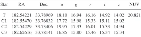
Table 1. SDSS coordinates and u, g,r, i,z magnitudes of the target SDSS 1210 and the comparison stars used in the analysis. We also pro-vide theGALEXNUV magnitude of SDSS 1210.

Star RA Dec. u g r i z NUV

T 182.54221 33.78969 18.10 16.94 16.16 14.92 14.02 20.821 C1 182.55470 33.76832 17.72 15.98 15.33 15.11 15.02 C2 182.54229 33.73406 19.95 17.33 16.01 15.33 14.94 C3 182.62616 33.78141 16.85 15.80 15.46 15.34 15.34

Table 1 lists the SDSS coordinates and magnitudes of SDSS 1210 and the three comparison stars used in the analysis presented in this paper, while Table 2 summarizes our photometric and spectroscopic observations. We note that SDSS 1210 has a Galaxy Evolution Explorer(GALEX; Morrissey et al. 2007) near-ultraviolet (NUV) detection, but no far-ultraviolet (FUV) detection.

2.1 Photometry: LT/RISE

Photometric observations were obtained with the robotic 2.0-m LT on La Palma, Canary Islands, using the high-speed frame-transfer CCD camera RISE (Steele et al. 2004) equipped with a single widebandV+Rfilter (Steele et al. 2008). Observations were carried out in 1-h blocks, using a 2×2 binning mode with exposure times of 5 s.

The data were de-biased and flat-fielded in the standard fashion within the LT reduction pipeline and aperture photometry was per-formed using SEXTRACTOR(Bertin & Arnouts 1996) in the manner described in G¨ansicke et al. (2004).

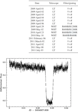
A sample light curve is shown in Fig. 1. The out-of-eclipse vari-ation is ellipsoidal modulvari-ation, arising from the tidally deformed secondary.

2.2 Spectroscopy: WHT/ISIS

Time-resolved spectroscopy was carried out at the 4.2-m William Herschel Telescope (WHT) on La Palma, Canary Islands, equipped with the double-armed Intermediate dispersion Spectrograph and Imaging System (ISIS). The spectrograph was used with a 1-arcsec slit, and an 600 lines mm−1 _{grating (R600B/R600R) on each of}

the blue and red arms, although a few spectra were obtained with a 1200 lines mm−1_{grating on the red arm (R1200R). Both the EEV12}

CCD on the blue arm and the REDPLUS CCD on the red arm were binned by three in the spatial direction and two in the spectral direction. This set-up resulted in an average dispersion of 0.88 Å per binned pixel over the wavelength range 3643–5137 Å (blue arm) and 0.99 Å per binned pixel over the wavelength range 7691– 9184 Å (red arm, R600R). From measurements of the full width at half-maximum of arclines and strong skylines, we determine the resolution to be 1.4 Å.

The spectra were reduced using the Starlink2_packages

KAPPAand

FIGAROand then optimally extracted (Horne 1986) using thePAMELA3

code (Marsh 1989). The wavelength scale was derived from copper– neon and copper–argon arc lamp exposures taken every hour during the observations, which we interpolated to the middle of each of the science exposures. For the blue arm the calibration was determined from a fifth-order polynomial fit to 25 lines, with a root mean square

2_{Maintained and developed by the Joint Astronomy Centre and available} from http://starlink.jach.hawaii.edu/starlink

3_{Available from http://www.warwick.ac.uk/go/trmarsh}

2011 The Authors, MNRAS419,817–826

(3)

[image:3.595.46.309.80.456.2]

SDSS 1210

+

3347

819

Table 2. Log of the photometric and spectroscopic observations. For the LT observations, we also provide the number of 1-h observing blocks per night.

Date Telescope Filter/grating Exp. (s) Blocks Frames Eclipses

2009 April 01 LT V+R 5 1 708 1

2009 April 02 LT V+R 5 2 1416 0

2009 April 03 LT V+R 5 2 1416 1

2009 April 04 LT V+R 5 2 1416 1

2009 April 05 LT V+R 5 3 2124 1

2009 April 06 LT V+R 5 1 708 0

2009 April 29 WHT R600B/R1200R 900 – 1 –

2009 May 02 WHT R600B/R1200R 900 – 3 –

2010 April 23 WHT R600B/R1200R 600 – 1 –

2010 May 18 WHT R600B/R600R 900 – 12 –

2011 February 06 LT V+R 5 1 720 1

2011 March 02 LT V+R 5 1 720 1

2011 April 02 LT V+R 5 1 720 1

2011 May 08 LT V+R 5 1 720 1

2011 July 03 LT V+R 5 1 720 1

Figure 1. Sample light curve of SDSS 1210 obtained with a 5-s cadence using RISE on the LT on 2009 April 05.

(rms) of 0.029 Å. The red arm was also fitted with a fifth-order polynomial, to 17 arclines. The rms was 0.032 Å.

3 O R B I TA L P E R I O D A N D E P H E M E R I S

We determined the orbital period and ephemeris of SDSS 1210 through mid-eclipse timings. This was achieved as follows.

Mid-eclipse times were measured by mirroring the observed eclipse profile around an estimate of the eclipse centre and shifting the mirrored profile against the original until the best overlap was found. This method is particularly well suited for the box-shaped eclipse profiles in (deeply) eclipsing PCEBs.

An initial estimate of the cycle count was then obtained by fitting eclipse phases (φobserved

0 −φfit0)−2over a wide range of trial periods.

Once an unambiguous cycle count was established, a linear fit, of the formT =T0 + PorbE, was performed to the times of mid-eclipse

[image:3.595.325.532.318.433.2]

versus cycle count, yielding a preliminary orbital ephemeris. Subsequently, we phase folded our data set using this preliminary ephemeris and proceeded with the light-curve model fitting (see Section 6). Having an accurate model at hand, we refitted each light curve individually. This provides a robust estimate of the error on

Table 3. Times of mid-eclipse (and their errors), O−C val-ues (and their errors) and cycle number for the ephemeris of SDSS 1210. Mid-eclipse times and errors are in MJD(BTDB), O−C values and errors are in seconds.

Mid-eclipse (d) Error (d) O−C (s) Error (s) Cycle

54923.0336744 0.0000060 −1 1 0

54925.0255324 0.0000082 1 1 16

54926.1459281 0.0000069 −0 1 25

54927.1418460 0.0000087 −0 1 33

55599.1376175 0.0000061 3 1 5431

55623.0396100 0.0000056 −1 1 5623

55654.0375754 0.0000081 −0 1 5872

55690.0151216 0.0000063 1 1 6161

55745.9109933 0.0000069 −2 1 6610

the mid-eclipse time, as our code includes the time of mid-eclipse T0as a free parameter.

Repeating the cycle count determination and the linear ephemeris fitting, as described above, we obtain the following ephemeris for SDSS 1210:

MJD (BTDB)=54923.033 686(6)+0.124 489 764(1)E, (1)

calculated on a Modified Julian Date-time-scale and corrected to the Solar system barycentre, with the numbers in parentheses indicating the error on the last digit. Thus, SDSS 1210 has an orbital period ofPorb=2.987 754 336(24) h. The mid-eclipse times, the observed

minus calculated values (O−C) and their respective errors are given in Table 3. Given the short baseline, there is as yet no evidence for period changes which are frequently seen in such binaries (e.g. Parsons et al. 2010b).

4 S P E C T R O S C O P I C A N A LY S I S

Although the SDSS spectrum of SDSS 1210 remained inconclu-sive with respect to the nature of the WD (Rebassa-Mansergas et al. 2010), our blue-arm WHT spectroscopy immediately revealed a host of narrow metal lines that exhibit radial velocity variations antiphased with respect to those of the M dwarf. The WHT spectra obtained in 2010 May, averaged in the WD rest frame and contin-uum normalized, are shown in Fig. 2 and illustrate the wealth of absorption lines from Mg, Al, Si, Ca, Mn and Fe. Similar metal

(4)

[image:4.595.45.285.56.237.2]

Figure 2. The normalized average WHT spectrum in the WD rest frame, along with line identifications for absorption lines originating in the WD photosphere.

lines have been detected in the optical spectra of a few other cool PCEBs, e.g. RR Cae (Zuckerman et al. 2003) or LTT 560 (Tappert et al. 2007), and indicate accretion of mass via a wind from the M dwarf.

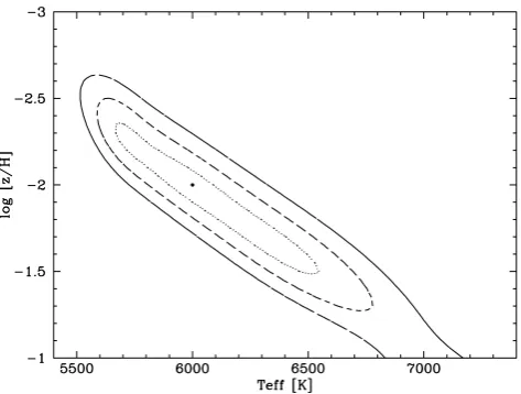
We have analysed the blue WHT spectra using hydrogen domi-nated but metal-polluted (DAZ) spectra calculated with the stellar atmosphere code described by Koester (2010). We fixed the surface gravity to logg=7.70, as determined from the fits to the LT light curve (Section 6). The model grid covered effective temperatures 5400 ≤ Teff,WD ≤ 7400 K in steps of 200 K and metal and He

abundances of log [Z/H]= −3.0,−2.3,−2.0,−1.3,−1.0, with all relevant elements up to zinc included, and fixed their relative abun-dances ratios to the respective solar values. We then fitted the model spectra to the average WHT spectrum in the range 3645–3930 Å, where the contribution of the M dwarf is entirely negligible. A good fit is found forTeff,WD 6000 K and metal abundances at0.01

their solar values, however, the effective temperature and the metal abundances are strongly correlated (Fig. 3).

Figure 3. Results of model spectra fitting to the average WHT spectrum. The single, big point indicates the best-fitting solution. The contours indicate the regions where theχ2_{of the fit is within 1, 2 and 3}_σ_{(dotted, short-dashed} and long-dashed lines, respectively) of the minimum (single point).

This degeneracy is lifted by including theGALEXdetection of SDSS 1210, as the predicted NUV flux is a strong function of the effective temperature. The uncertainty in the absolute flux calibra-tions of our WHT spectra and theGALEXobservations introduces a small systematic uncertainty on the final result, and we settle forTeff,WD = 6000±200 K and log [Z/H]= −2.0± 0.3.

Inde-pendently, the weakness of the Balmer lines in the WHT spectrum also requires thatTeff,WD 6400 K. The spectral modelling of

SDSS 1210 is illustrated in Fig. 4.

Adopting the WD radius from the light-curve fit (Sections 6 and 7),RWD = 0.0159 R, the flux-scaling factor of the best-fitting

spectral model implies a distance ofd50±5 pc, which is in good agreement withd∼66±34 pc estimated by Rebassa-Mansergas et al. (2010) from fitting the M dwarf.

The detection of metals in the photosphere of the WD allows an estimate of the accretion rate (e.g. Dupuis et al. 1993; Koester & Wilken 2006), as long as the system is in accretion–diffusion equilibrium. In cool, hydrogen-rich atmospheres, such as the one in SDSS 1210, the diffusion time-scales of the different metals de-tected in the WHT spectrum vary by a factor of∼2 for a given temperature, and are, forTeff,WD = 6000 K, in the range 30 000–

60 000 yr.4_{It is plausible to assume that the average accretion rate}

over the diffusion time-scales involved is constant, as the binary configuration (separation of the two stars, Roche lobe filling factor of the companion) changes on much longer time-scales. Summing up the mass fluxes at the bottom of the convective envelope, and taking into account the uncertainties inTeff,WDand the metal

abun-dances, gives ˙M(5±2)×10−15_M

yr−1_{. There are now three}

PCEBs with similar stellar components that have measured accre-tion rates: RR Cae ( ˙M4×10−16_M

yr−1_{; Debes 2006); LTT 560}

( ˙M 5×10−15_M

yr−1_{; Tappert et al. 2011) and SDSS 1210}

( ˙M5×10−15_M

yr−1_).

Although SDSS 1210 and LTT 560 have similar orbital periods, the period of RR Cae is roughly twice as long, suggesting that the efficiency of wind accretion decreases as the binary separation and Roche lobe size of the companion increase, as is expected. A more systematic analysis of the wind-loss rates of M dwarfs and the efficiency of wind accretion in close binaries would be desirable, but will require a much larger sample of systems.

5 T H E S P E C T R O S C O P I C O R B I T

Radial velocities of the binary components have been measured from the FeIλλ4045.813, 4063.594, 4071.737, 4132.058, 4143.869 absorption lines for the WD and the NaIλλ8183.27, 8194.81 ab-sorption doublet for the secondary star.

The FeIlines were simultaneously fitted with a second-order polynomial plus five Gaussians of common width and a separation fixed to the corresponding laboratory values. A sine fit to the radial velocities phase folded using the orbital ephemeris (equation 1) yieldsKWD=95.3±2.1 km s−1andγWD=24.2±1.4 km s−1.

The NaIdoublet was fitted with a second-order polynomial plus two Gaussians of common width and a separation fixed to the cor-responding laboratory value. A sine fit to the radial velocities phase

4_{For completeness, we note that because we have adopted solar abundance} ratios for the metals, these small differences in diffusion time-scales imply slightly non-solar ratios in the accreted material. In principle, the individual metal-to-metal ratios can be determined from the observed spectrum of the WD, and hence allow us to infer the abundances of the companion star, however, this requires data with substantially higher spectral resolution to resolve the line blends.

[image:4.595.46.283.507.686.2]

(5)

[image:5.595.67.534.56.414.2]

SDSS 1210

+

3347

821

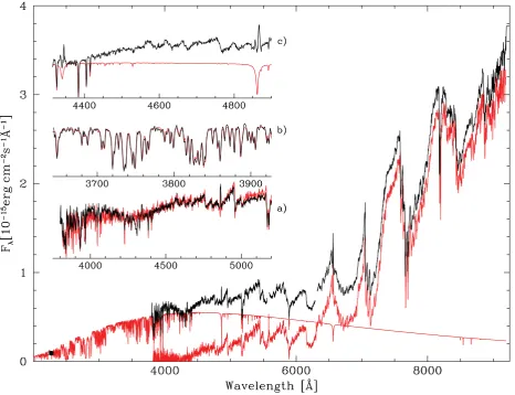
Figure 4.Spectral modelling of SDSS 1210. Main panel: the SDSS spectrum (black) and theGALEXNUV flux (black point), along with the best-fitting WD model (red∗,Teff,WD=6000 K, logg=7.70, log [Z/H]= −2.0) and the best-fitting M-dwarf template for the companion (red∗, spectral type M5). Inset (a): the sum of the WD model and M-dwarf template provide a good match to the blue end of the SDSS spectrum (black), with the low flux of the M-dwarf template being the dominant limitation. Inset (b): best-fitting WD model (red∗) and the average WHT spectrum forλ <3930 Å, where the M dwarf contributes practically nothing to the observed flux. Inset (c): best-fitting WD model (red∗) and the average WHT spectrum (black) illustrating the weakness of the Hβ and Hγlines of the WD. Increasing the temperature very rapidly results in Balmer lines and/or a NUV flux that are inconsistent with the observations.∗The coloured figure is available in the online version only.

folded using the orbital ephemeris yieldsKsec=251.7±2.0 km s−1

andγsec=12.2±0.9 km s−1.

Fig. 5 shows the measured radial velocities phase folded on the orbital period and the corresponding sine fits.

Knowledge of both radial velocities allows us to obtain the mass ratioqof the binary, namelyq=KWD/Ksec =0.379±0.009. We

tentatively interpret the difference betweenγWD andγsec as the

gravitational redshift of the WDzWD,spec, which yieldszWD,spec =

11.9±1.7 km s−1_{(see also Section 7).}

6 L I G H T- C U RV E M O D E L L I N G

To obtain the stellar parameters of the binary components, light-curve models were fitted to the data usingLCURVE(see Copperwheat et al. 2010 for a description, as well as Pyrzas et al. 2009; Parsons et al. 2010a, 2011 for further applications).

6.1 Code input

The code computes a model based on input system parameters supplied by the user. The physical parameters defining the models

Figure 5. Phase-folded radial velocity curves of the secondary star (filled circles) and the WD (open circles), with their respective errors. Also shown are the sine fits to the velocities of both components. A full cycle is repeated for clarity.

[image:5.595.309.550.508.687.2]

(6)

are (i) the mass ratioq=Msec/MWD, (ii) the binary inclinationi,

(iii) the stellar radii scaled by the binary separationrWD=RWD/a

andrsec=Rsec/a, (iv) the unirradiated stellar temperaturesTeff,WD

andTsec, (v) the sum of the unprojected stellar orbital speedsVS=

(KWD + Ksec)/sini, (vi) the time of mid-eclipse of the WDT0,

(vii) limb- and gravity-darkening coefficients and (viii) the distance d. The code accounts for the distance simply as a scaling factor that can be calculated very rapidly for any given model, and so it does not enter the optimization process. All other parameters can be allowed to vary during the fit.

6.2 Free and fixed parameters

During the minimization, we keptTeff,WDfixed atTeff,WD=6000 K.

The gravity darkening of the secondary was also kept fixed at 0.08 (the usual value for a convective atmosphere). Limb-darkening co-efficients were also held fixed. For the WD we calculated quadratic limb-darkening coefficients from a WD model with Teff,WD =

6000 K and logg= 7.70, folded through the RISE filter profile. The corresponding values were found to bea= 0.174 andb= 0.421 forI(μ)/I(1)=1−a(1−μ)−b(1−μ)2_{, with}_μ_{being the}

cosine of the angle between the line of sight and the surface normal. For the secondary star we used the tables of Claret & Bloemen (2011). We interpolated between the values ofVandRfor aT = 3000 K and logg=5 star, to obtain quadratic limb-darkening coef-ficientsa=0.62 andb =0.273. All other parameters were allowed to vary.

6.3 Minimization

Initial minimization is achieved using the downhill-simplex and Levenberg–Marquardt methods (Press 2002), while the Markov chain Monte Carlo (MCMC) method (Press et al. 2007) was used to determine the distributions of our model parameters (e.g. Ford 2006, and references therein).

The MCMC method involves making random jumps in the model parameters, with new models being accepted or rejected according to their probability computed as a Bayesian posterior probability (the probability of the model parameters, θ, given the data, D, P(θ|D)).P(θ|D) is driven by a combination ofχ2_{and a prior}

prob-ability, P(θ), that is based on previous knowledge of the model parameters.

In our case, the prior probabilities for most parameters are as-sumed to be uniform. The photometric data provide constraints for the radii and inclination angle, however, the photometry alone can-not constrain the masses, as the light curve itself is only weakly depended onq. To alleviate this, we can use our knowledge ofKWD

andKsec. At each jump, the model valuesKmWD andK m

sec are

cal-culated throughq,iandVS.P(θ) is then evaluated on the basis of

the observedKWD andKsec, assuming a Gaussian prior probability P(μ,σ2_{), with}_μ_and_σ _{corresponding to the measured values and}

errors ofKWD andKsec.

A crucial practical consideration of MCMC is the number of steps required to fairly sample the parameter space, which is largely determined by how closely the distribution of parameter jumps matches the true distribution. We therefore built up an estimate of the correct distribution starting from uncorrelated jumps in the parameters, after which we computed the covariance matrix from the resultant chain of parameter values. The covariance matrix was then used to define a multivariate normal distribution that was used to make the jumps for the next chain. At each stage the actual size of the jumps was scaled by a single factor set to deliver a

model acceptance rate of≈25 per cent (Roberts, Gelman & Gilks 1997). After three such cycles, the covariance matrix showed only small changes, and at this point we carried out the long ‘production runs’ during which the covariance and scalefactor which define the parameter jumps were held fixed.

6.4 Stellar parameters

Using the following set of equations, the stellar and binary param-eters are obtained directly from the posterior distribution of the model parameters, as output from the MCMC minimization.

The binary separation is obtained from the model parameterVS

through

a= Porb

2π VS. (2)

The WD and secondary masses are obtained from the model pa-rametersqandVS as

MWD= Porb

2πG 1 1+ qVS

3 ₍₃₎

and

Msec= Porb

2πG

q

1+ qVS

3_. ₍₄₎

The stellar radii are directly obtained from the model parameters rWD andrsec and equation (2) and the surface gravity of the WD is

of course given by

logg=log

_GM WD R2 WD . (5)

6.5 Intrinsic data uncertainties

The acquisition of high-precision absolute photometry on the LT in service mode is somewhat difficult to achieve. Each observing block individually covered only a third of the orbital phase and the blocks were obtained over many nights, under varying conditions (seeing, sky brightness, extinction, airmass). The data are sensitive to changes in conditions, as they have been obtained through the very broad and non-standardV+Rfilter of RISE. In the absence of a flux standard, the photometry cannot be calibrated in absolute terms. When phase folding the LT data, significant scatter is found at orbital phases where individual observing blocks with discrepant calibrations contribute. This affects both the shape of the eclipse, mainly the steepness of the WD ingress/egress and, to a lesser ex-tend, the eclipse duration, and the out-of-eclipse variation, i.e. the profile of the ellipsoidal modulation. As a result, there is an unavoid-able systematic uncertainty in the photometric accuracy of our data, which will influence the determination of the stellar parameters.

To gauge the effect of the systematic uncertainties we worked in the following fashion: each observing block has been reduced thrice, each time using one of the three comparison stars reported in Table 1. C1 has ag−rcolour index comparable to SDSS 1210, C2 is fairly red, while C3 is fairly blue. The data of each reduction were then phase folded together and two light curves were produced: one containing all the photometric points and one where (2–3) observing blocks with an obviously large intrinsic scattering were omitted. Thus, we ended up with six phase-folded light curves. A dedicated MCMC optimization was calculated for each light curve. We will use the following notation when referring to these chains: C1A denotes a light curve produced with comparison star C1 and all datapoints, C2E denotes a light curve produced with comparison star C2 excluding observing blocks and so on.

(7)

SDSS 1210

+

3347

823

7 R E S U LT S

The results of the six MCMC processes are summarized in Table 4. The quoted values and errors are purely of statistical nature and represent the mean and rms of the posterior distribution of each parameter. The radius of the secondary, as determined byrsec and a, is measured along the line connecting the centres of the two stars

and, due to the tidal distortion, its value is larger than the average radius. Therefore, in Table 4 we also report the more representative value of the volume-averaged radius.

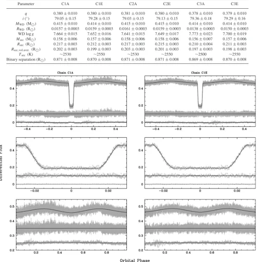
[image:7.595.49.552.183.694.2]

To illustrate the achieved quality of the fits, we plot models C1A and C1E in Fig. 6. While the overall quality of the fit is very satisfactory, the model seems to slightly overpredict the flux at the ‘wings’ of the ellipsoidal modulation profile (phases∼0.05–0.15

Table 4. Stellar and binary parameters obtained from MCMC optimization. The quoted values and errors are the mean and rms of the posterior distribution of each parameter. The chains represent light curves created using comparison stars C1, C2 or C3 and either including all (A) observing blocks or excluding (E) those with obviously large scattering. See text for details.

Parameter C1A C1E C2A C2E C3A C3E

q 0.380±0.010 0.380±0.010 0.381±0.010 0.380±0.010 0.378±0.010 0.379±0.010

i(◦) 79.05±0.15 79.28±0.15 79.03±0.15 79.13±0.15 79.36±0.18 79.29±0.16

MWD(M) 0.415±0.010 0.414±0.010 0.415±0.010 0.415±0.010 0.414±0.010 0.414±0.010

RWD (R) 0.0157±0.0003 0.0159±0.0003 0.0161±0.0003 0.0159±0.0003 0.0138±0.0003 0.0150±0.0003 WD logg 7.664±0.015 7.652±0.016 7.641±0.015 7.649±0.017 7.773±0.023 7.700±0.019

Msec (M) 0.158±0.006 0.157±0.006 0.158±0.006 0.158±0.006 0.156±0.007 0.157±0.006

Rsec (R) 0.217±0.003 0.212±0.003 0.217±0.003 0.215±0.003 0.210±0.004 0.211±0.003

Rsec,vol.aver. (R) 0.202±0.003 0.199±0.003 0.203±0.003 0.201±0.003 0.197±0.003 0.198±0.003

Tsec (K) ∼2530 ∼2550 ∼2530 ∼2550 ∼2500 ∼2550 Binary separation (R) 0.871±0.008 0.870±0.008 0.871±0.008 0.871±0.008 0.869±0.008 0.870±0.008

Figure 6.Light-curve fitting results for models C1A (left) and C1E (right). In each of the six panels we plot the phase folded light curve with the model superimposed (top trace), the residuals of the fit (middle trace, offset from 0 for clarity) and a binned version of the residuals (bottom trace). Shown are the entire light curve (top panels), a zoom around the eclipse (middle panels) and the out-of-eclipse ellipsoidal modulation (bottom panels).

(8)

and∼0.85–0.95). This discrepancy could be data related, due to the intrinsic scattering of points; system related, due to the presence of starspots affecting the modulation; model related, as the treatment of stellar temperatures is based on blackbody spectra, for one specific wavelength; or due to a combination of these factors.

With regard to the binary and stellar parameters, the MCMC results indicate the following: as expected for a detached system, the light curves depend very weakly on qand its value is well constrained by the radial velocities. All six chains give inclination angle values just above 79◦, consistent with each other within the errors. There is a slight shift upwards when excluding blocks from the phase folded light curve.

The tight spectroscopic constraints mean that the component masses are largely independent of the model/data set used. Thus, the WD in SDSS 1210 has a mass ofMWD= 0.415±0.010 M

and the secondary star a mass ofMsec=0.158±0.006 M.

The quantity most seriously affected by systematics is the WD radius. This is especially evident when considering models C3A and C3E. However, such a discrepancy is expected, since C3 is considerably bluer than SDSS 1210 and is more susceptible to air-mass/colour effects, leading to large intrinsic scattering. The values forRWD as obtained from C1A, C1E, C2A and C2E are consistent

within their errors, indicating a systematic uncertainty comparable to the statistical one. This is illustrated in Fig. 7.

[image:8.595.307.544.54.235.2]

The secondary star radius is affected in a similar, albeit less pronounced, way. All six models lead to values broadly consistent within their statistical errors and a systematic uncertainty of the same order as the statistical one. Fig. 8 shows the six different values of the volume-averaged secondary star radius overplotted on aM–R relation for MS stars. Taken at face value, the results of the MCMC optimization indicate that the secondary is∼10 per cent larger than theoretically predicted. As can be seen in Fig. 8, this discrepancy

[image:8.595.44.282.424.596.2]

Figure 7. M–Rplot for WDs. Black points are data from Provencal et al. (1998), Provencal et al. (2002) and Casewell et al. (2009). The dotted line is the zero-temperatureM–Rrelation of Eggleton as quoted in Verbunt & Rappaport (1988). The dashed line, marked as (He,6) is a M–R re-lation for aTeff,WD = 6000 K, He-core WD, with a hydrogen layer of M(H)/MWD=3×10−4, interpolated from the models of Althaus & Ben-venuto (1997). NN Ser (Parsons et al. 2010a) is marked, along with the track forTeff,WD=60000 K, C/O core WD,M(H)/MWD=10−4(long dash–dot line), indicating the accuracy achieved in eclipsing PCEBs. The results of the six chains for SDSS 1210 are plotted in red (online version only). In-set panel: zoom-in on the values of SDSS 1210. The points are C1A: open circle; C1E: filled circle; C2A: open square; C2E: filled square; C3A: open triangle; C3E: filled triangle.

Figure 8. M–Rplot for low-mass stars. Black points are data from L´opez-Morales (2007) and Beatty et al. (2007), where the masses of single stars were determined using mass–luminosity relations. The dotted line is the 5.0-Gyr isochrone from Baraffe et al. (1998). The dashed line is a 5.0-Gyr model including effects of magnetic activity from Morales et al. (2010). The results of the six chains for the volume-averaged radius of the secondary in SDSS 1210 are plotted in red (online version only). Inset panel: zoom-in on the values of SDSS 1210. The points are C1A: open circle; C1E: filled circle; C2A: open square; C2E: filled square; C3A: open triangle; C3E: filled triangle.

drops to∼5 per cent, if magnetic activity of the secondary is taken into account. With regard to the secondary temperature, we note again that due to the blackbody approximation, the value ofTsec

does not necessarily represent the true temperature of the star, it is effectively just a flux-scaling factor.

The gravitational redshift predicted by the light-curve models (Table 4), correcting for the redshift of the secondary star, the dif-ference in transverse Doppler shifts and the potential at the sec-ondary star owing to the WD, arezWD= 15.9±0.4 km s−1from

C1E andzWD = 15.8±0.4 km s−1 from C2E, where the errors

are purely statistical and have been derived in the same manner as the other quantities reported in Table 4. The systematic uncertain-ties in our photometric data might still be influencing the result, as the inclination angle and the stellar radii enter the calculation of zWD. ComparingzWD with the spectroscopically determined value

ofzWD,spec=γWD −γsec=11.9±1.7 km s−1we find that they are

consistent within∼2σ. The systemic velocitiesγWD andγsec are

determined from spectroscopic observations obtained using a dual-arm spectrograph, with the WD velocity measured in the blue dual-arm and that of the secondary measured in the red arm (Sections 2 and 5). The observations in both arms are independently wavelength calibrated and the rms of∼0.03 Å (Section 2) corresponds to an accuracy of the zero-point of∼1–2 km s−1_{. The potential of an}

off-set in the calibrations of the two arms enters the determination of zWD,spec as an additional systematic uncertainty.

8 PA S T A N D F U T U R E E VO L U T I O N O F S D S S 1 2 1 0

Considering its short orbital period, SDSS 1210 must have formed through common-envelope evolution (Paczynski 1976; Webbink 2008; see also Nordhaus et al. 2010 for the additional effects of tidal interaction). As shown by Schreiber & G¨ansicke (2003), if the binary and stellar parameters are known, it is possible to

(9)

SDSS 1210

+

3347

825

reconstruct the past and predict the future evolution of PCEBs for a given angular momentum loss prescription. Here, we assume clas-sical disrupted magnetic braking (Verbunt & Zwaan 1981). In this context, given the low mass of the secondary, the only angular mo-mentum loss mechanism for SDSS 1210 is gravitational radiation. Based on the temperature and the mass of the WD we interpolate the cooling tracks of Althaus & Benvenuto (1997) and obtain a cooling age oftcool = 3.5 Gyr. This corresponds to the time that

passed since the binary left the common envelope. We calculate the period it had when it left the common envelope to bePCE =

4.24 h. Following the same method as in Zorotovic et al. (2010) and based on their results we reconstructed the initial parameters of the binary using a common-envelope efficiency ofαCE=0.25 and the

same fraction of recombination energy (see Zorotovic et al. 2010, for more details). We found an initial mass ofMprog = 1.33 M

for the progenitor of the WD, which filled its Roche lobe when its radius wasRprog = 91.3 R. At that point, the orbital separation

wasa= 162.7 R, and the age of the system wastsys=4.4 Gyr,

since the time it was formed. Using the radius of the secondary5

we calculate that the system will reach a semidetached configura-tion and become a cataclysmic variable (CV) at an orbital period of Psd∼2 h intsd=1.5 Gyr.

Given that the currentPorb places SDSS 1210 right at the upper

edge of the CV orbital period gap,6 _{and that the calculated}_P

sd,

when SDSS 1210 will start mass transfer, is right at the lower edge of the period gap, we are tempted to speculate whether SDSS 1210 is in fact a detached CV entering (or just having entered) the period gap. Davis et al. (2008) have shown that a large number of detached WD+MS binaries with orbital periods between 2 and 3 h are in fact CVs that have switched off mass transfer and are crossing the period gap. This could in principle explain the apparently oversized secondary in SDSS 1210, as expected from the disrupted magnetic braking theory (e.g. Rappaport, Verbunt & Joss 1983). However, the temperature of the WD in SDSS 1210 seems to be uncomfortably low for a WD that has recently stopped accreting (Townsley & G¨ansicke 2009).

9 D I S C U S S I O N A N D C O N C L U S I O N S

In this paper, we have identified SDSS 1210 as an eclipsing PCEB containing a very cool, low-mass, DAZ WD and a low-mass MS companion.

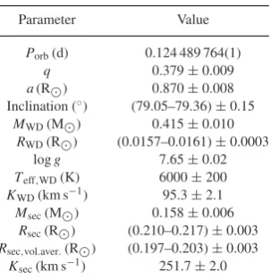
Using combined constraints from spectroscopic and photometric observations we have managed to measure the fundamental stellar parameters of the binary components. Systematic uncertainties in the absolute calibration of our photometric data influence the de-termination of the stellar radii. The stellar masses, however, remain unaffected and were measured to a 1 per cent accuracy. The (formal) statistical uncertainties in all binary parameters indicate the level of precision that can be achieved in this system. All parameters are summarized in Table 5.

With a mass ofMWD=0.415±0.010 Mand a temperature of Teff,WD ∼ 6000 K, the DAZ WD in SDSS 1210 pushes the

bound-aries in a hitherto unexplored region of the WD parameter space. The M–Rresults from the four chains C1 and C2 are consistent with a He-core WD, assuming a hydrogen layer ofM(H)/MWD=3×10−4.

However, due to lack of observational constraints for the H-layer

5_{We assume a representative value of}_R

sec,vol.aver.=0.2 Rfor the volume-averaged radius of the secondary.

[image:9.595.354.506.78.235.2]

6_{The orbital period range where only a small number of CVs are found.}

Table 5.Adopted stellar and binary parameters for SDSS 1210.

Parameter Value

Porb(d) 0.124 489 764(1)

q 0.379±0.009

a(R) 0.870±0.008 Inclination (◦) (79.05–79.36)±0.15

MWD(M) 0.415±0.010

RWD(R) (0.0157–0.0161)±0.0003

logg 7.65±0.02

Teff,WD(K) 6000±200

KWD(km s−1) 95.3±2.1

Msec(M) 0.158±0.006

Rsec(R) (0.210–0.217)±0.003

Rsec,vol.aver.(R) (0.197–0.203)±0.003

Ksec(km s−1) 251.7±2.0

thickness and the uncertainty in the radii, we will defer identify-ing the WD as a definite He core and simply emphasize the strong candidacy.

The secondary star, with a mass ofMsec =0.158±0.006 M,

illustrates once more the excellent opportunity that PCEBs give us for testing and calibrating theM–Rrelations of low-mass stars. Tak-ing the radius measurements at face value, the secondary star seems to be∼10 per cent larger than the theoretical values, although this drops to∼5 per cent, if magnetic activity is taken into considera-tion. In this context, the magnetic activity present in the secondary can lead to the formation of stellar (dark) spots on the surface. The effect of these spots is to block the outgoing heat flux, reducingTeff

and, as a result, the secondary expands to maintain thermal equilib-rium (Chabrier, Gallardo & Baraffe 2007; Morales et al. 2010). A further∼2 per cent inflation could be attributed to tidal and rota-tional deformation (Sirotkin & Kim 2010; see also Knigge, Baraffe & Patterson 2011). Kraus et al. (2011) found that low-mass stars in short-period binaries appear to be overinflated (although their analysis was restricted to Msec > 0.3 M), which seems to be

the case for SDSS 1210. We should note, however, that the mass and radius of the secondary star in the eclipsing PCEB NN Ser (withMsec =0.111±0.004 Mand comparable orbital period to

SDSS 1210) are consistent with theoreticalM–Rpredictions, even though it is heavily irradiated by the hot WD primary (Parsons et al. 2010a).

We have speculated whether SDSS 1210 is in fact a detached CV entering the period gap, which could explain the large radius of the secondary. This hypothesis could be tested by measuring the rotational velocity of the WD. This can be achieved through high-resolution spectroscopy of the FeIabsorption lines in the WD photosphere (see e.g. Tappert et al. 2011).

In any case, it is highly desirable to improve the measurement of the stellar radii in SDSS 1210 to the comparable precision to the masses presented here. This will require high-precision photometry in standard filters, such as e.g. delivered by ULTRACAM (Dhillon et al. 2007).

AC K N OW L E D G M E N T S

We thank the anonymous referee for a prompt report. BTG, TRM, EB and CMC are supported by an STFC Rolling Grant. MRS and AR-M acknowledge financial support from FONDECYT in the form of grants 1100782 and 3110049. MZ acknowledges sup-port from Gemini/CONICYT (grant 32100026). Based in part on

(10)

observations made with the William Herschel Telescope operated on the island of La Palma by the Isaac Newton Group in the Spanish Observatorio del Roque de los Muchachos of the Instituto de As-trof´ısica de Canarias and on observations made with the Liverpool Telescope operated on the island of La Palma by Liverpool John Moores University in the Spanish Observatorio del Roque de los Muchachos of the Instituto de Astrof´ısica de Canarias with financial support from the UK Science and Technology Facilities Council.

R E F E R E N C E S

Abazajian K. N. et al., 2009, ApJS, 182, 543 Adelman-McCarthy J. K. et al., 2008, ApJS, 175, 297 Althaus L. G., Benvenuto O. G., 1997, ApJ, 477, 313 Andersen J., 1991, ARA&A, 3, 91

Baraffe I., Chabrier G., Allard F., Hauschildt P. H., 1998, A&A, 337, 403 Bayless A. J., Orosz J. A., 2006, ApJ, 651, 1155

Beatty T. G. et al., 2007, ApJ, 663, 573 Berger D. H. et al., 2006, ApJ, 644, 475 Bertin E., Arnouts S., 1996, A&AS, 117, 393

Brown W. R., Kilic M., Hermes J. J., Allende Prieto C., Kenyon S. J., Winget D. E., 2011, ApJ, 737, 23

C¸ akırlı ¨O., Ibanoˇglu C., 2010, MNRAS, 401, 1141

Casewell S. L., Dobbie P. D., Napiwotzki R., Burleigh M. R., Barstow M. A., Jameson R. F., 2009, MNRAS, 395, 1795

Chabrier G., Gallardo J., Baraffe I., 2007, A&A, 472, L17 Claret A., Bloemen S., 2011, A&A, 529, A75

Copperwheat C. M., Marsh T. R., Dhillon V. S., Littlefair S. P., Hickman R., G¨ansicke B. T., Southworth J., 2010, MNRAS, 402, 1824

Davis P. J., Kolb U., Willems B., G¨ansicke B. T., 2008, MNRAS, 389, 1563 Debes J. H., 2006, ApJ, 652, 636

Dhillon V. S. et al., 2007, MNRAS, 378, 825

Dimitrov D. P., Kjurkchieva D. P., 2010, MNRAS, 406, 2559 Drake A. J. et al., 2010, preprint (arXiv:1009.3048)

Dupuis J., Fontaine G., Pelletier C., Wesemael F., 1993, ApJS, 84, 73 Ford E. B., 2006, ApJ, 642, 505

G¨ansicke B. T., Araujo-Betancor S., Hagen H.-J., Harlaftis E. T., Kitsionas S., Dreizler S., Engels D., 2004, A&A, 418, 265

Horne K., 1986, PASP, 98, 609 Irwin J. et al., 2010, ApJ, 718, 1353

Knigge C., Baraffe I., Patterson J., 2011, ApJS, 194, 28 Koester D., 2010, Mem. Soc. Astron. Ital., 81, 921 Koester D., Wilken D., 2006, A&A, 453, 1051

Kraus A. L., Tucker R. A., Thompson M. I., Craine E. R., Hillenbrand L. A., 2011, ApJ, 728, 48

L´opez-Morales M., 2007, ApJ, 660, 732 Marsh T. R., 1989, PASP, 101, 1032

Morales J. C., Ribas I., Jordi C., 2008, A&A, 478, 507 Morales J. C. et al., 2009, ApJ, 691, 1400

Morales J. C., Gallardo J., Ribas I., Jordi C., Baraffe I., Chabrier G., 2010, ApJ, 718, 502

Morrissey P. et al., 2007, ApJS, 173, 682

Nebot G´omez-Mor´an A. et al., 2009, A&A, 495, 561

Nordhaus J., Spiegel D. S., Ibgui L., Goodman J., Burrows A., 2010, MNRAS, 408, 631

Paczynski B., 1976, in Eggleton P., Mitton S., Whelan J., eds, Proc. IAU Symp. 73, Structure and Evolution of Close Binary Systems. Reidel, Dordrecht, p. 75

Panei J. A., Althaus L. G., Benvenuto O. G., 2000, A&A, 353, 970 Parsons S. G., Marsh T. R., Copperwheat C. M., Dhillon V. S., Littlefair S.

P., G¨ansicke B. T., Hickman R., 2010a, MNRAS, 402, 2591 Parsons S. G. et al., 2010b, MNRAS, 407, 2362

Parsons S. G., Marsh T. R., G¨ansicke B. T., Drake A. J., Koester D., 2011, ApJ, 735, L30

Press W. H., 2002, Numerical Recipes in C++: The Art of Scientific Com-puting. Cambridge Univ. Press, Cambridge

Press W. H., Teukolsky A. A., Vetterling W. T., Flannery B. P., 2007, Nu-merical Recipes. The Art of Scientific Computing, 3rd edn. Cambridge Univ. Press, Cambridge

Provencal J. L., Shipman H. L., Hog E., Thejll P., 1998, ApJ, 494, 759 Provencal J. L., Shipman H. L., Koester D., Wesemael F., Bergeron P., 2002,

ApJ, 568, 324

Pyrzas S. et al., 2009, MNRAS, 394, 978

Rappaport S., Verbunt F., Joss P. C., 1983, ApJ, 275, 713

Rebassa-Mansergas A., G¨ansicke B. T., Schreiber M. R., Koester D., Rodr´ıguez-Gil P., 2010, MNRAS, 402, 620

Rebassa-Mansergas A., Nebot Gómez-Morán A., Schreiber M. R., Girven J., Gänsicke B. T., 2011, MNRAS, 413, 1121

Ribas I., 2006, Ap&SS, 304, 89

Roberts G. O., Gelman A., Gilks W. R., 1997, Ann. Applied Probability, 7, 110

Schreiber M. R., G¨ansicke B. T., 2003, A&A, 406, 305

Schreiber M. R., G¨ansicke B. T., Southworth J., Schwope A. D., Koester D., 2008, A&A, 484, 441

Sirotkin F. V., Kim W.-T., 2010, ApJ, 721, 1356 Southworth J., Clausen J. V., 2007, A&A, 461, 1077 Steele I. A. et al., 2004, Proc. SPIE, 5489, 679

Steele I. A., Bates S. D., Gibson N., Keenan F., Meaburn J., Mottram C. J., Pollacco D., Todd I., 2008, in McLean I. S., Casali M. M., eds, Proc. SPIE Vol. 7014, Ground-based and Airborne Instrumentation for Astronomy II. SPIE, Bellingham, p. 217

Steinfadt J. D. R., Kaplan D. L., Shporer A., Bildsten L., Howell S. B., 2010, ApJ, 716, L146

Tappert C., G¨ansicke B. T., Schmidtobreick L., Aungwerojwit A., Mennick-ent R. E., Koester D., 2007, A&A, 474, 205

Tappert C., G¨ansicke B. T., Schmidtobreick L., Ribeiro T., 2011, A&A, 523, 129

Torres G., 2007, ApJ, 671, L65

Townsley D. M., G¨ansicke B. T., 2009, ApJ, 693, 1007 Verbunt F., Rappaport S., 1988, ApJ, 332, 193 Verbunt F., Zwaan C., 1981, A&A, 100, L7

Webbink R. F., 2008, in Milone E. F., Leahy D. A., Hobill D. W., eds, Astrophys. Space Sci. Library, Vol. 352, Short-Period Binary Stars: Observations, Analyses and Results. Springer, Berlin, p. 233

Wood M. A., 1995, in Koester D., Werner K., eds, Lecture Notes in Physics, Vol. 443, White Dwarfs. Springer-Verlag, Berlin, p. 41

York D. G. et al., 2000, AJ, 120, 1579

Zorotovic M., Schreiber M. R., Gänsicke B. T., Nebot Gómez-Morán A., 2010, A&A, 520, A86

Zuckerman B., Koester D., Reid I. N., H¨unsch M., 2003, ApJ, 596, 477

This paper has been typeset from a TEX/LA_{TEX file prepared by the author.}