Multi Objective Optimal Dispatch Considering Wind Power and Interactive Load for Power System

(1)

ISSN Online: 1947-3818 ISSN Print: 1949-243X

DOI: 10.4236/epe.2018.104B001 Apr. 11, 2018 1 Energy and Power Engineering

Multi-Objective Optimal Dispatch Considering

Wind Power and Interactive Load for Power

System

Xinxin Shi

1,2,3

_{, Guangqing Bao}

1,2,3*

_{, Kun Ding}

4

_{, Liang Lu}

4

1_{College of Electrical and Information Engineering, Lanzhou University of Technology, Lanzhou, China}

2_{Key Laboratory of Gansu Advanced Control for Industrial Processes, Lanzhou University of Technology, Lanzhou, China}

3_{National Demonstration Center for Experimental Electrical and Control Engineering Education, Lanzhou University of}

Technology, Lanzhou, China

4_{Key Laboratory of Wind Power Integration Operation and Control, Gansu Electric Power Corporation Wind Power Corporation}

Wind Power Technology Center, Lanzhou, China

Abstract

With the rapid and large-scale development of renewable energy, the lack of new energy power transportation or consumption, and the shortage of grid peak-shifting ability have become increasingly serious. Aiming to the severe wind power curtailment issue, the characteristics of interactive load are stu-died upon the traditional day-ahead dispatch model to mitigate the influence of wind power fluctuation. A multi-objective optimal dispatch model with the minimum operating cost and power losses is built. Optimal power flow dis-tribution is available when both generation and demand side participate in the resource allocation. The quantum particle swarm optimization (QPSO) algo-rithm is applied to convert multi-objective optimization problem into single objective optimization problem. The simulation results of IEEE 30-bus system verify that the proposed method can effectively reduce the operating cost and grid loss simultaneously enhancing the consumption of wind power.

Keywords

Wind Power, Interactive Load, Optimal Dispatch, Multi-Objective, QPSO Models

1. Introduction

Wind power industry has been rapidly developed. Wind power generation reached 241 billion kW∙h that has been 30% year-on-year growth accounting for How to cite this paper: Shi, X.X., Bao,

G.Q., Ding, K. and Lu, L. (2018) Mul-ti-Objective Optimal Dispatch Considering Wind Power and Interactive Load for Power System. Energy and Power Engi-neering, 10, 1-10.

https://doi.org/10.4236/epe.2018.104B001

(2)

DOI: 10.4236/epe.2018.104B001 2 Energy and Power Engineering

4% of the total electricity generation in China. Among them, new energy in-stalled capacity accounted for more than 30% of the total inin-stalled capacity of the local power supply in Gansu, Ningxia, Xinjiang, Qinghai, which has shown favourable prospects in reducing fossil energy consumption and pollutant emis-sions [1]. However, the demand of electricity is influenced by variable factors, such as weather, economy, laws, policies, electrical load conditions, and so on. These factors make electric dispatch became a task. Especially, when the wind power integrated into the main grid, the intermittent and stochastic nature of such energy brings challenges to system dispatch. Therefore, usage of wind power generation is of major importance in future power grids for economic and environmental reasons. In recent years, the researches of academic experts published which classified into two major categories, one is multi-objective dis-patch modeling; another one is optimal disdis-patch solving technology. A stochas-tic multi-objective optimal reactive power dispatch model is studied concerning about load and wind power generation uncertainties, including real power losses and operation cost of wind farms [2]. The objective function is implemented for energy saving and emission-reduction [3]. The day-ahead multi-objective op-timal dispatching model containing thermal power, hydro power, wind-power and pumped storage units is given to minimize the total costs and CO2 emission

under multiple constraints. A fuzzy modeling for dynamic economic dispatch is presented in [4], which could make the dispatch to reflect the willingness of de-cision-makers and hereby adapt the random wind power output better. A mul-ti-objective optimization algorithm based on the non-dominated sorting diffe-rential evolution is used to solve the economic environmental dispatch stochas-tic optimization model of power system connected with large scale wind farms [5]. And a solution of optimal dispatch problem with a particle swarm optimisa-tion based on multi-agent systems is presented in [6]. Optimal scheduling strat-egy is considered only from the generation side above literature. In this paper, the characteristics of interaction load and integration into the traditional sche-duling model is discussed. The problem is formulated as a multi-objective op-timal problem through simultaneous minimizing both system operational cost and power loss. QPSO algorithm has been introduced to solve this problem. Fi-nally, the system simulation is carried out with IEEE 30 nodes. The experimental results verify the effectiveness of the proposed method, and have some certain practical significance for power system optimal scheduling.

2. Interactive Load Modeling

1) Interactive load characteristics 2) Interactive load model

• _{Shiftable load}

(3)

the peak. Therefore, for the rth shiftable load, the decision variable is the start variable t

sr

U : If it starts in the t period, then t 1 sr

U = ; If it starts at other times, then Utsr=0; tsr is the start time of the rth shiftable peak load [7] [8].

The shift cost curve characterizes denotes the compensation price that the us-er should obtain from the grid company aftus-er providing the shift sus-ervice. The mathematical description is as follows:

0 0

0 0 0

( ) 0

( )

0

sr sr sr

t

sr sr sr sr sro sr sr

sr sr sr

m t t t t

C m t t m T t t T

t t t T

 − ≤ <



=_ − − > +

 _{≤ ≤} ₊



(1)

where is t sr

C the peak cost of the rth shiftable peak load in the t_{period of the} peak; msr is the compensation factor for the load of the rth shiftable peak load

that is determined by the load control agreement signed from the user and the power company in advance; tsr₀ and Tsr₀ are the number of the original power load start time and load duration before the peak which belong to known para-meters.

• _{Interruptible load}

Users through the auction to declare interruptible capacity and compensation prices as well as the dispatch center by calculating the optimal power generation scheduling program to determine the interruptible users and the optimal capac-ity. Dispatching the hth interruptible load of the user’s compensation cost as shown in Equation (4) [9]

0

t t t

Ih Ih Ih Ih

C =C P I (2)

where CIh0 is the unit to reduce load costs of the hth interruptible load in the

contract; t Ih

P is the load reduction of the hth interruptible load in the tperiod ; and t

Ih

I is variable dispatch for interruptible load. The interruptible load was whether to dispatched basing on t 1

Ih

I = and t 0 Ih

I = .

3. Multi-Objective Optimal Statement

The problem of economic power dispatch with wind penetration consideration can be formulated as a multi-objective optimal dispatch model. The two con-flicting objectives, i.e., operating cost and system power loss, should be mini-mized simultaneously while fulfilling certain system constraints. This problem is formulated mathematically in this section.

3.1. Problem Objectives

• _{Objective 1: Minimization of operational cost}

1

minC =CGi+CWi (3)

}

{

2 1

1 1

[ ( ) ] (1 )

c

N T

t t t t t t

Gi Gi i i Gi i Gi Ui Gi Ri

t i

C U a b P c P C U− C

= =

=

∑∑

+ + + − + (4)

1 1 1

( )

S I

N N

T

t t

Wi Sr Ih

t j i

C C C

= = =

(4)

where T is the number of hours during system dispatching; NC is the number

of generating units; and t Gi

P , t Gi

U are the active output and the state variables of the ith generator in the period; indicates a shutdown state. On the contrary, t 1

Gi

U = indicates that the generator set is on; t Ri

C , t Ui

C denote the spare costs and starting cost of the ith generator in the period; NS, NI

represent the number of shiftable peak load; t Sr

C , t Ih

C denote the cost of the rth removable peak load and the hth interruptible load in the t period.

• _{Objective 2: Minimization of system power loss}

The dispatch of interactive load will inevitably cause the change of power flow distribution, which will have some influence on the system power loss. Thus, the minimize of power loss is one goal of optimal dispatching. Here the use of

B-coefficient method to calculate the power loss [10].

2 , ,0 0,0

1 1 1 1

min ( )

T K K K

t t t

i i j j i i

t i j i

C P B P B P B

= = = =

=

∑ ∑∑

+

∑

+ ₍₆₎

where K is the number of system nodes; Bi j, ,Bi,0,B0,0 are the second term ,

which are the first term and the constant term of the coefficient; and t i

P , P_jt

are active power of node i and j.

3.2. Problem Constraints

• _{Constraint 1: Power balance constraint [11]}

• _{Constraint 2: Spare constraints}

• _{Constraint 3: Unit constraint}

• _{Constraint 4: Interactive load constraint [12]}

3.3. Optimal Dispatch Modeling

The objective of this model is to minimize the operating cost and the grid loss as much as possible under all constraints. Therefore, when the operating cost and the network loss are lower, the fitness value of the fitness function is greater. Where the fitness function can be defined as [13]:

2 1

( ) 0

i x

i i i x i x i

i x i

C C

C C mC n C C C C

C C C

µ

≤ 



=_ + + < ≤ + ∆

 _> _{+ ∆}



(7)

2

( 2 _x _i _i 1) / _i

m= − C∆ − ∆C C − ∆C (8)

2 2

1 _x _x [( 2 _x _i _i 1) / _i]

n= −C −C ⋅ − C∆ − ∆C C − ∆C (9)

i i x

C C C

∆ = − (10)

where Ci is the ith objective function value; Cx is the ith objective function

ideal value. ∆Ci is the ith objective function added value. The fitness function

diagram is shown in Figure 1.

Thus, where the fitness index can be defined as:

{

1 2

}

min (C), (C )

µ= µ µ (11)

t t 0

Gi

U =

(5)

[image:5.595.300.444.74.152.2]

Figure 1. Fitness function diagram.

where µ is the minimum value for all fitness functions.

The multi-objective problem is transformed into a single objective nonlinear optimization problem that satisfies the fitness value of all constraints:

1 1 1 1

2 2 2 2

max . .

s t C C C C

C C C C

µ µ

µ

+ ∆ ≤ + ∆

(12)

4. Proposed Approach

In this paper, the quantum particle swarm optimization (QPSO) [14] is used to solve the model, which is based on the particle swarm optimization (PSO) to improve the formation. All particles in the population are treated as quantum particles in the feasible solution. When updating the particle position, it mainly considers the current local optimal position and global optimal position infor-mation of each particle.

5. Simulation and Evaluation

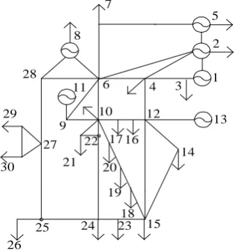
In this study, a IEEE 30-bus system with 1-wind farm of grid-connected is used to investigate the effectiveness of the model. The system configuration is shown in Figure 2.

The system parameters including generator capacities, spare cost and fuel cost coefficients are listed in Table 1.

The interruptable capacity, compensation price, interruptable times and dura-tion for interruptible load are listed in Table 2.

1) There are 100 wind turbines in the wind farm with a total installed capacity of 200 MW. Conventional unit positive and negative rotation standby demand for the maximum unit capacity of 15%.

2) The particle size scale of QPSO algorithm is 100 and the maximum number of iterations is 500.

3) The prediction curves and load forecast curves of the wind power during the last 24 hours are shown in Figure 3.

4) The willingness curve and the peak cost of the shiftable load are shown in Figure 4 and Figure 5, respectively.

(6)

[image:6.595.289.458.74.254.2]

[image:6.595.262.487.284.393.2]

Figure 2. Wiring diagram of IEEE 30-bus system.

[image:6.595.206.538.445.532.2]

Figure 3. Day-ahead wind power and load prediction curve.

Table 1. Data of conventional generator.

Unit No.

Power generation cost

factor Spare cost factor Output limit Up/down Output

ai bi ci di ei PGi,up PGi,down PGi,max PGi,min

1(1) 786.1 38.4 0.152 16 19 50 50 200 50 2(5) 1048.9 40.3 0.028 13 12 15 15 60 15 3(13) 1355.2 38.1 0.018 9 10 15 15 40 15

Table 2. Data of interruptible loads.

No. PIH /MW λHK/[$/(MW∙h)] Times TIH,cont/h

1(7) 4.3 10 2 2

2(19) 2.2 5 2 2

3(21) 3.6 8 2 4

Table 3. Results of multi-objective optimization.

µ µ(C₁) µ(C2) C1 C2

0.434 0.870 0.434 636147 147.95

0.513 0.846 0.513 636652 144.12

0.695 0.832 0.695 636946 130.17

0.826 0.828 0.826 637030 129.47

26

1 2 5 7

8

4 3

28

6

9 11

27 29

30 21

22

20

19

18

25 24 23 15

14 13 12

17 16 10

0 4 8 12 16 20 24

0 50 100 150 200 250 300 350

P/

W

M

t/h

Load predition

[image:6.595.209.538.562.619.2] [image:6.595.209.538.652.724.2]

(7)

[image:7.595.258.487.76.322.2]

Figure 4. Shiftable load curves.

Figure 5. Cost curve of shiftable loads.

Figure 4 and Figure 5 are, respectively, the time and peak load cost curve. Through reasonable optimization calculations, interruptible load 1, 2, 3 and shiftable load 1, 2 are put into the system; although the shiftable load capacity of the load 3 is relatively large, but because of its shiftable capacity and peak surge costs will be increased system operating cost. It does not meet the economic needs of the operation of the grid, so it does not work. It can be seen from Table 3, the system operating cost of $637030 when the equal to 0.826 which the net loss is 129.47 MW. It can be seen that the power system which integrates the in-teractive load can provide more reserve for the power grid with wind farm and it reduce the impact of wind power randomness. While reducing the switching costs of interactive load make the power grid more economical and reliable op-eration.

The results are compared using the conventional optimal scheduling model and the interactive load multi-objective optimal scheduling model. Figure 6 and Figure 7 are the two models of the output curve, respectively.

It can be seen from Figure 6 and Figure 7 that the traditional optimal sche-duling model usually need to reduce the output of the conventional unit in the wind power generation period or increasing the output of the conventional unit in the lesser period of wind power. This leads that the conventional unit's output curve isn’t better. Thus, the normal unit 1 and 2 must be worked to meet the system peak demand. But the interactive load multi-objective optimal scheduling model reduces the valley difference of the system. Therefore, it is not necessary that make the normal unit 2 to work.

In the following, the results of the traditional optimization scheduling model and the multi-objective optimization scheduling model considering the interactive

0 2 4 6 8 10 12 14 16

0 2 4 6

P

/MW

t/h

shiftable load 1 shiftable load 2 shiftable load 3

0 4 8 12 16 20 24

0 5 10 15 20 25 30

C/

$

t/h

(8)

[image:8.595.258.488.77.179.2] [image:8.595.262.485.216.321.2]

Figure 6. Output curve of traditional scheduling model.

[image:8.595.207.539.375.426.2]

Figure 7. Output curve of optimal dispatching model.

Table 4. Total operational cost of system.

Calculation Generation Spare Interactive total

Traditional 585909 69818 0 655727

[image:8.595.206.538.461.512.2]

Optimization 541285 21218 74527 637030

Table 5. Grid loss of system.

Calculation method Power loss /MW

Traditional model 139.06

Optimization model 129.47

load are compared in Table 4 and Table 5.

It can be seen from Table 4 and Table 5 that the shiftable load is better for shifting peak in power system. It is put into the system scheduling system, which can improve the operational efficiency of power systems and decrease the grid loss of system. The generating units are run at a cost-effective level by reducing the frequent shutdown of the generating units. In addition, the interruption load can also reduce the cost of spare capacity due to the random fluctuations in wind power. Compared with the traditional optimal scheduling model, the total sys-tem power generation cost and grid loss of syssys-tem are reduced.

6. Conclusion

The operation cost of power grid will become increased when the capacity of wind power which have fluctuation and randomness is increased. The solution

0 4 8 12 16 20 24

0 5 10 15 20 25

P

/MW

t/h

traditional unit 1 traditional unit 2 traditional unit 3

0 4 8 12 16 20 24

0 5 10 15 20 25

P

/M

W

(9)

of this problem is the interactive load which is adjusted the power grid to inte-ract with user. The inteinte-ractive load decreased the operation cost because it can be a part of the reserve capacity of electric power system. In addition, on the ba-sis that bring the interaction load into the optimal scheduling of the system which include the wind farm, a multi-objective optimization scheduling model based on the minimum operation cost and network loss are established. A quantum particle swarm optimization (QPSO) algorithm is utilized to solve the optimization objective of the model which achieve minimum of system power loss and operational cost. Simulation results show the interactive load’s ability to reduce the cost of reserve capacity due to the random fluctuations in wind pow-er. Experimental results demonstrated that the model was successfully imple-mented.

Acknowledgements

The authors would like to thank the financial support from National Natural Science Foundation of China (51267011), and partly financed by Gansu Electric Power Research Institute (271733-KJ-07).

References

[1] Sun, B., Yu, Y.X. and Qin, C. (2017) Should China Focus on the Distributed

Devel-opment of Wind and Solar Photovoltaic Power Generation? A Comparative Study.

Applied Energy, 185, 421-439.https://doi.org/10.1016/j.apenergy.2016.11.004

[2] Mohseni-Bonab, S.M. and Rabiee, A. (2017) Optimal Reactive Power Dispatch: A

Review and a New Stochastic Voltage Stability Constrained Multi-Objective Model

at the Presence of Uncertain Wind Power Generation. IET Generation,

Transmis-sion & Distribution, 11, 815-829.https://doi.org/10.1049/iet-gtd.2016.1545

[3] Shi, N., Zhou, S.Q., Su, X.W., et al. (2016) Unit Commitment and Multi-Objective

Optimal Dispatch Model for Wind-Hydro-Thermal Power System with Pumped

Storage. 2016 IEEE 8th International Power Electronics and Motion Control

Confe-rence (IPEMC-ECCE Asia).

[4] Chen, H.Y., Chen, J.F. and Duan, X.Z. (2009) Fuzzy Modeling and Optimization

Algorithm on Dynamic Economic Dispatch in Wind Power Integrated System.

Pro-ceeding of the CSEE, 29, 13-17.

[5] Sun, H.J., Peng, C.H. and Yi, H.J. (2012) Multi-Objective Stochastic Optimal

Dis-patch of Power System. Electric Power Automation Equipment, 32, 123-128.

[6] Zhao, B., Guo, C. and Cao, Y. (2005) A Multiagent-Based Particle Swarm

Optimiza-tion Approach for Optimal Reactive Power Pispatch. IEEE Trans. Power Syst, 20,

1070-1078.https://doi.org/10.1109/TPWRS.2005.846064

[7] Graditi, G., Di Silvestre, M.L., et al. (2014) Heuristic-Based Shiftable Load Optimal

Management in Smart Micro-Grids. IEEE Transactions on Industrial Informatics,

11, 271-280.https://doi.org/10.1109/TII.2014.2331000

[8] Cakmak, R. and Altas, I.H. (2016) Scheduling of Domestic Shiftable Loads via

Cuckoo Search Optimization Algorithm. 2016 4th International Istanbul Smart Grid

Congress and Fair (ICSG).

[9] Wang, Q.Q., Zhao, C.H., Ma, C.F., et al. (2011) Scheduling of Interruptible Load

(10)

Univer-DOI: 10.4236/epe.2018.104B001 10 Energy and Power Engineering

sity Engineering and Technology Edition, 11, 19-25.

[10]Guo, Z.Z., Wu, J.K. and Kong, F. (2013) Multi-Objective Optimization Scheduling

for Hydrothermal Power Systems Based on Electromagnetism-Like Mechanism and

Data Envelopment Analysis. Proceedings of the CSEE, 33, 53-61.

[11]Suzuki, H. (2014) Dynamics of Load Balancing with Constraints. The European

Physical Journal: Special Topics, 223, 2631-2635.

https://doi.org/10.1140/epjst/e2014-02278-7

[12]Wang, B.B., Liu, X.C. and Li, Y. (2013) Day-Ahead Generation Scheduling and

Op-eration Simulation Considering Demand Response in Large-Capacity Wind Power Integrated Systems. Proceedings of the CSEE, 33, 35-44.

[13]Wu, J.K, and Tang, L. (2012) Stochastic Optimization Scheduling Method for

Hy-drothermal Power Systems with Stochastic Loads. Proceedings of the CSEE, 32,

36-43.

[14]Sun, J. and Xu, W.B. (2004) A Global Search Strategy of Quantum-Behaved Particle

Swarm Optimization. Proceedings of IEEE Conference on Cybernetics and