White Rose Research Online URL for this paper:
http://eprints.whiterose.ac.uk/120257/
Version: Accepted Version
Article:
Allison, R.J., Goodwin, S.P., Parker, R.J. et al. (2 more authors) (2010) The early
dynamical evolution of cool, clumpy star clusters. Monthly Notices of the Royal
Astronomical Society, 407 (2). pp. 1098-1107. ISSN 0035-8711
https://doi.org/10.1111/j.1365-2966.2010.16939.x
[email protected]
https://eprints.whiterose.ac.uk/
Reuse
Unless indicated otherwise, fulltext items are protected by copyright with all rights reserved. The copyright
exception in section 29 of the Copyright, Designs and Patents Act 1988 allows the making of a single copy
solely for the purpose of non-commercial research or private study within the limits of fair dealing. The
publisher or other rights-holder may allow further reproduction and re-use of this version - refer to the White
Rose Research Online record for this item. Where records identify the publisher as the copyright holder,
users can verify any specific terms of use on the publisher’s website.
Takedown
If you consider content in White Rose Research Online to be in breach of UK law, please notify us by
arXiv:1004.5244v1 [astro-ph.GA] 29 Apr 2010
The early dynamical evolution of cool, clumpy star clusters
Richard J. Allison
1, Simon P. Goodwin
1⋆, Richard J. Parker
1,
Simon F. Portegies Zwart
2, and Richard de Grijs
3,11 Department of Physics and Astronomy, University of Sheffield, Sheffield, S3 7RH, UK 2 Leiden Observatory, Leiden University, PO Box 9513, 2300 RA Leiden, The Netherlands 3 Kavli Institute for Astronomical Astrophysics, Peking University, Beijing 100871, China
ABSTRACT
Observations and theory both suggest that star clusters form sub-virial (cool) with highly sub-structured distributions. We perform a large ensemble of N-body simu-lations of moderate-sized (N = 1000) cool, fractal clusters to investigate their early dynamical evolution. We find that cool, clumpy clusters dynamically mass segregate on a short timescale, that Trapezium-like massive higher-order multiples are com-monly formed, and that massive stars are often ejected from clusters with velocities
>10 km s−1 (c.f. the average escape velocity of 2.5 km s−1). The properties of
clus-ters also change rapidly on very short timescales. Young clusclus-ters may also undergo core collapse events, in which a dense core containing massive stars is hardened due to energy losses to a halo of lower-mass stars. Such events can blow young clusters apart with no need for gas expulsion. The warmer and less substructured a cluster is initially, the less extreme its evolution.
Key words: methods:N-body simulations - stars: formation - stars: kinematics and dynamics
1 INTRODUCTION
Most stars appear to form in star clusters (Lada & Lada 2003; Lada 2009; Portegies Zwart et al. 2010) and so star formation is inextricably linked with star cluster formation. Recent advances in observations and theory have allowed us to construct a basic picture of cluster formation in which clusters form dynamically cool (virial), and highly sub-structured.
Clusters form in highly turbulent molecular clouds. These clouds are highly substructured, containing dense clumps and filaments (Williams 1999; Williams et al. 2000; Carpenter & Hodapp 2008) which are presumably formed by the decay of supersonic turbulence (Mac Low & Klessen 2004; Ballesteros-Paredes et al. 2007). Stars and small stel-lar groups form in these dense regions and are unsur-prisingly observed to have a high degree of substructure when young (Larson 1995; Elmegreen 2000; Testi et al. 2000;
Cartwright & Whitworth 2004; Gutermuth et al. 2005;
Allen et al. 2007; Schmeja & Klessen 2006; Schmeja et al. 2008), clustering in young stellar groups has even been observed in the SMC (Schmeja et al. 2009) and LMC (Bastian et al. 2009). The same behaviour is seen in sim-ulations of cluster formation (Klessen & Burkert 2000, 2001; Bate et al. 2003; Bonnell et al. 2003; Bate 2009;
⋆ E-mail: [email protected]
Offner et al. 2009), including in comparison tests between AMR and SPH techniques (Federrath et al. 2010).
Clusters are observed to lose their substructure as they evolve, becoming smooth and roughly spherical (Cartwright & Whitworth 2004; Schmeja & Klessen 2006; Schmeja et al. 2008). Goodwin & Whitworth (2004) have shown that substructure can only be erased in clus-ters if the clusclus-ters are initially cool (sub-virial) (see also Maschberger et al. 2010). Both observations of pre-stellar cores (Belloche et al. 2001; Andr´e 2002; Walsh et al. 2004; Peretto et al. 2006; Kirk et al. 2007) and stars (Peretto et al. 2006; Proszkow et al. 2009) show that they indeed appear to be sub-virial, a property also found in simulations of cluster formation (Klessen & Burkert 2000; Offner et al. 2009; Maschberger et al. 2010).
Following Allison et al. (2009b) we conduct N-body
2 INITIAL CONDITIONS
We perform 160 N-body simulations with 1000 stars each,
in which the initial conditions are cool and clumpy. We vary the level of substructure and initial virial ratio, and conduct ensembles of simulations with the same initial conditions, varying only the initial random number seed used to ini-tialise the simulations.
To create initial substructure in our simulations we use a fractal stellar distribution. Using a fractal distri-bution provides a parameterisation of substructure using only a single number: the fractal dimension. (Note that we are not claiming that clusters are actually initially frac-tal, although they may be (Elmegreen & Elmegreen 2001; Cartwright & Whitworth 2004), just that this provides a simple descriptor of substructure that is easy to reproduce). The fractal stellar distributions were generated fol-lowing the method of Goodwin & Whitworth (2004). The
method begins by defining a cube of side Ndiv (we use
Ndiv = 2 throughout), inside of which the fractal will be
built. A first-generation parent is placed at the centre of the
cube, from which are spawned N3
div sub-cubes, each
con-taining a first-generation child in its centre. The fractal is then built by determining which of the children themselves become parents, and spawn their own offspring. This is
de-termined by the fractal dimension, D, where the
probabil-ity that a child becomes a parent is Ndiv(D−3). For a lower
fractal dimension less children will mature and so the final distribution will contain more structure. Any children which do not become parents in a given step are removed, along with all of their parents. A small amount of noise is then added to the positions of the remaining children, prevent-ing the final cluster from havprevent-ing a gridded appearance, and the children become parents of the next generation. Each
new parent then spawnsN3
divsecond-generation children in
Ndiv3 sub-sub-cubes, with each second-generation child
hav-ing a Ndiv(D−3) probability of becoming a second-generation
parent. This process is then repeated until there are substan-tially more children than required. The children are pruned to produce a sphere from the cube and are then randomly removed (so maintaining the fractal dimension) until the required number of children are left. These children then become the stars in the cluster.
To determine the velocity structure of the cloud, chil-dren inherit their parent’s velocity plus a random component that decreases with each generation in the fractal. The chil-dren of the first generation are given random velocities from
a Gaussian of mean zero1. Each new generation then
inher-its their parent’s velocity plus an extra random component that becomes smaller with each generation. This results in a velocity structure in which nearby stars have similar ve-locities, but distant stars can have very different velocities. Finally, the velocity of every star is scaled to obtain the desired total virial ratio for the cluster.
The simulations contain 1000 stars, have an initial
max-1 Here the variance is unimportant as the velocities are scaled to the desired virial ratio once the final spatial distribution is obtained, but the method can also be used to match the Larson (1981) relations if desired (see Goodwin & Whitworth 2004).
D
Q 1.6 2.0 2.6 3.0
0.3 a1.01–50 a2.01–10 a3.01–10 a4.01–10 0.4 b1.01–10 b2.01–10 b3.01–10 b4.01–10 0.5 c1.01–10 c2.01–10 c3.01–10 c4.01–10
Table 1.Notation for run identification whereD is the initial fractal dimension, andQis the initial virial ratio of each simu-lation. The numbers 01–50 and 01–10 are the identifiers for each individual run. Within each ensemble only the random number seed used to generate the initial conditions is changed.
imum radius of 1 pc, include no primordial binaries or gas and a three-part power law is used to produce an initial mass function (IMF, Kroupa 2002),
N(M)∝
( M−0.3 m
06M/M⊙< m1, M−1.3 m
16M/M⊙< m2, M−2.3 m
26M/M⊙< m3,
(1)
with m0 = 0.08 M⊙, m1 = 0.1 M⊙, m2 = 0.5 M⊙ and
m3 = 50 M⊙. No stellar evolution is included because of
the short duration of the simulations (∼ 4 Myr). We use
thestarlabN-body integratorkirato run our simulations
(Portegies Zwart et al. 2001).
In this study we explore a range of fractal dimensions and virial ratios. The fractal dimensions investigated are
D = 1.6, 2.0, 2.6 and 3.0 (since these values correspond
to the number of maturing children,ND
div ≡2D , being an
integer), whereD = 1.6 produces a large amount of
struc-ture, andD= 3.0 produces a uniform sphere. We investigate
virial ratios ofQ= 0.3, 0.4 and 0.5, we define the virial
ra-tio asQ=T /|Ω|(whereT and|Ω|are the total kinetic and
total potential energy of the stars, respectively), hence virial
equilibrium isQ= 0.5.
It is important to note that fractal initial conditions are inherently stochastic: statistically identical fractals (i.e., the same fractal dimension), can appear very different to the eye, and can evolve in very different ways (see Section 3.3). Therefore, it is vital to perform large ensembles of simula-tions with different random number seeds. We have therefore
simulated 50D = 1.6,Q= 0.3 (a1) clusters (as they have
the most interesting evolution), and restricted our analysis
of all other combinations of D and Q to 10 clusters each.
The identifiers and initial conditions of each ensemble are presented in table 1.
To quantify mass segregation we use the minimum span-ning tree (MST) method (Allison et al. 2009a). This method
compares the MST of theNmost massive stars with the
av-erage MSTs ofNrandomly selected stars. The ratio of these
two MST lengths gives a quantitative measure of the con-centration of the massive stars and hence a value of the mass segregation in the cluster,
Λ = hlnormi
lmassive
± σnorm
lmassive
(2)
where Λ is the measure of mass segregation,hlnormi is the
average length of the random MSTs,lmassiveis the length of
the massive star MST andσnormis the error in the random
MST length. The valueσnorm/lmassiveis the 1σerror in Λ.
the simulation) in all three dimensions. We note that an observer will see only two dimensions, and may not iden-tify all cluster members, in particular low-mass stars and stars that have been ejected from the cluster. Allison et al. (2009a) show that there is little difference between the mass segregation measure in two and three dimensions when us-ing mass segregated Plummer spheres. However, as with all mass segregation measures, if using the measure in two di-mensions projection effects may cause differences depending on orientation. Unfortunately, this is unavoidable. Including all stars is useful theoretically, however it does not allow a direct comparison with observational data.
3 RESULTS
3.1 Rapid dynamical mass segregation
In Allison et al. (2009b, hereafter Paper I) we showed that
cool (Q= 0.3), and clumpy (D= 1.6) clusters can
dynami-cally mass segregate on a timescale close to the initial
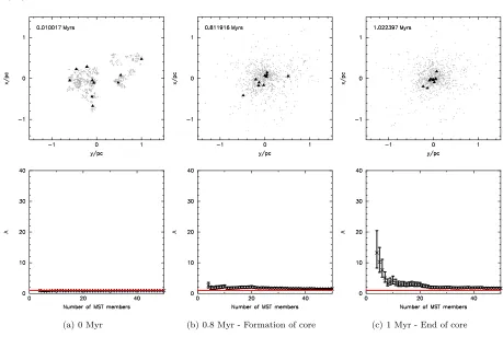
cross-ing time of the system (∼1 Myr). Figure 1 shows the early
evolution and onset of mass segregation in such a cluster. The top panels show the spatial distributions of the cluster
at times ∼ 0.01,0.81 and 1.02 Myr (left to right), whilst
the lower panels show the mass segregation ratio Λ for each of these snapshots – the higher the value of Λ, the greater the degree of mass segregation. As is clear from the figure, the cluster evolves from an initially non-mass segregated and clumpy distribution, into a smooth and mass segregated one. In paper I we argued that this rapid dynamical mass segregation is due to the collapse of the cool cluster
form-ing a very dense, but short-lived core (at∼0.8 Myr in the
example shown in Fig. 1). These dense cores (forD = 1.6,
Q= 0.3) tend to contain about half of the mass of the
clus-ter, are roughly 0.1 – 0.2 pc in radius, and survive for 0.1 –
0.2 Myr (10 – 20 crossing times in the core).
Spitzer (1969) showed that the timescale for mass
seg-regation,tseg, for a star of massM depends on how massive
that star is relative to the average mass of a star in a cluster,
hmi,
tseg(M)≈
hmi
M trelax, (3)
wheretrelaxis the relaxation time of the cluster, which
is related to its crossing time,tcross, by
trelax≈ N
8 lnNtcross. (4)
Eq. 3 can be rewritten as
tseg≈hmi M
N
8 lnNtcross. (5)
For the D = 1.6, Q = 0.3 initial conditions used in
paper I, typical values for these parameters are N ∼ 300
– 500, tcross ∼0.01 – 0.2 Myr,hmi ∼0.4 M⊙ (typical for
standard IMFs). The core has a lifetime of 0.1 – 0.2 Myr in
which it can mass segregate giving a mass to which the core
can segregate ofM ∼2 – 4 M⊙. In Fig. 1 the cluster is mass
segregated to the 20th most massive star, which has a mass
of a few M⊙, in good agreement with our simple analytical
model.
The reason that a dense core can form is that the cluster
is both coolandclumpy: cool clusters will initially collapse,
but cool and clumpy clusters can collapse further. The
po-tential energy, Ω, of a cluster of mass Mclus and radius R
is
Ω =−ηGM
2 clus
R , (6)
where η is a structure parameter whose value depends
on the choice of R (e.g., is it the core radius or the
half-mass radius?), and the structure of the cluster (e.g., is it clumpy, Plummer, or uniform density?) (see also, Portegies Zwart et al. 2010). For example, for a Plummer
sphere, ifRis the Plummer radius thenη∼0.3.
If a cluster has an initial potential energy Ω0 (with
ra-diusR0 and structure parameter η0), and an initial virial
ratioQ0, then the initial total energyE0 is
E0=−η0GM 2 clus R0
(1−Q0).
Whatever the initial conditions, a (bound) cluster will attempt to reach virial equilibrium and a relaxed configura-tion (something like a Plummer sphere, or King profile with
a concentration parameter2 ≈2−3, for an a1 type cluster).
Therefore, the final energyEf of the cluster (with potential
energy Ωf, radius Rf, structure parameter ηf, and virial
ratioQf = 0.5) will be
Ef =−ηf
1 2
GMclus2 Rf
(assuming no mass is lost). Equating these equations gives the degree of collapse (or expansion if initially warm) of the cluster
R0 Rf
=η0
ηf
2(1−Q0). (7)
Clearly, to induce dynamical mass segregation on a
short timescale,R0/Rf must be as large as possible to cause
the maximum degree of collapse. This implies that both
η0/ηf and 2(1−Q0) need to be large.
Obviously, making 2(1−Q0) large means makingQ0
as small as possible, but even with an initially static stellar
distribution with Q0 = 0, 2(1−Q0) can never be greater
than two (this is why Bonnell & Davis 1998 did not see rapid, early mass segregation). Realistically, it is difficult to
imagineQ0being much less than 0.2 or 0.3 as the starsmust
initially have some relative velocities.
As stated above, the cluster will not just relax into virial equilibrium, it will also attempt to reach a basic statistical equilibrium which is a smooth, centrally concentrated dis-tribution (like a Plummer sphere or King model if tidally truncated). Therefore the final structure parameter will be
ηf ∼0.3 when the scale radius is the Plummer radius.
Numerical experiments we have carried out show that
the structure parameter for a fractal of dimensionD= 1.6
is η0 ∼ 1.1±0.1, for D = 2.0, η0 ∼ 0.8±0.1 (note that
different realisations ofD= 1.6 andD= 2.0 fractals have a
large variation in their structure parameters), forD = 2.6,
η0 ∼ 0.7, and for D = 3.0,η0 ∼0.6. For each of these η
values the scale radius is the total radius of the fractal.
Un-fortunately, it is very difficult to exactly compare theη of
(a) 0 Myr (b) 0.8 Myr - Formation of core (c) 1 Myr - End of core
Figure 1.Run a1.34 –Top:2 dimensional stellar distributions at (a) 0 Myrs - the initial distribution, (b) 0.8 Myrs - the formation of the dense core and (c) 1 Myr - the end of the dense core and initial dynamical mass segregation. Triangles indicate the positions of the 10 most massive stars.Bottom:The evolution of Λ withNfor (a), (b), (c); as described above. The error bars show 1σdeviations.
a Plummer model and the η of a fractal as the radii are
defined differently. The half-mass radius of fractal models varies quite significantly (and its meaning is also rather un-clear in a fractal) and so does not provide a useful compar-ison radius either.
3.2 Mass segregation in clusters with different D
and Q
The analysis above suggests that the initial virial ratio and the initial fractal dimension of a cluster are the crucial pa-rameters in determining whether that cluster will be able to rapidly dynamically mass segregate. In particular, the
warmer (higher-Q), and the smoother (higher-D) a cluster
is, the lower the maximum central density, and hence less dynamical mass segregation will occur.
In Fig. 2 we show the typical evolution of Λ with time for clusters with different initial virial ratios and fractal
dimen-sions for N = 10,20 and 50, the full version of this figure,
showing the evolution of all of the simulations, can be found in the supplementary data. In the top left is our canonical
Q= 0.3, D= 1.6 cluster from paper I. From left to right,
the initial virial ratio increases from Q = 0.3 to 0.4 and
0.5 (virialised). From top to bottom, the fractal dimension
increases from D = 1.6 (very clumpy) to 2.0,2.6 and 3.0
(roughly a uniform density sphere).
It would be expected from our earlier argument that
lower-Qand lower-Dclusters will collapse to a denser state,
and hence show more rapid and more pronounced dynamical
mass segregation. This is exactly what is seen in Fig. 2: faster and more intense mass segregation at the top left (cool and clumpy clusters), and no appreciable mass segregation at all at the bottom right (virialised, uniform density clusters). The trend in the typical evolution of clusters in our param-eter space shown in Fig. 2 is exactly what we would expect to see following the theoretical argument in Section 3.1.
Whilst the behaviour of ‘typical’ clusters is exactly what is expected, many individual clusters show unusual and un-expected behaviour. Examination of each simulation (see the supplementary data) shows that, whilst the general pattern
of evolution withDand Qholds, there is a large degree of
stochasticity due to each fractal being different in detail to every other fractal.
3.3 Stochasticity
The supplementary data shows that a number of simulations do not show the behaviour that we might expect for their
D and Qvalues. The evolution of fractal clusters depends
(a)D= 1.6;Q= 0.3 – a1.21 (b)D= 1.6;Q= 0.4 – b1.05 (c)D= 1.6;Q= 0.5 – c1.06
(d)D= 2.0;Q= 0.3 – a2.08 (e)D= 2.0;Q= 0.4 – b2.08 (f)D= 2.0;Q= 0.5 – c2.06
(g)D= 2.6;Q= 0.3 – a3.04 (h)D= 2.6;Q= 0.4 – b3.02 (i)D= 2.6;Q= 0.5 – c3.09
[image:6.612.65.529.81.732.2](j)D= 3.0;Q= 0.3 – a4.02 (k)D= 3.0;Q= 0.4 – b4.03 (l)D= 3.0;Q= 0.5 – c4.03
There are several D= 1.6, Q= 0.3 clusters which ap-pear to have little or no mass segregation, for example run a1.20 (see Fig. 3). In this cluster there appears to be no sig-nificant mass segregation at any time during the 4 Myr of
the simulation for N = 10,20 and 50. Fig. 3(b) shows the
evolution of Λ for run a1.20 in more detail than Fig. 3(a). In
this plot we show Λ forN = 4,6,8,10 and 12. It is now clear
that the clusterdoesmass segregate, but only for stars more
massive than the 6th most massive star. In fact, a
substan-tial multiple system consisting of the 4 most massive stars is formed in this cluster. Mass segregation is only present
for the 6thmost massive stars because the 7thmost massive
star is ejected early in the simulation, thereby enlarging the length of all MSTs that include more than 7 stars. Mass
segregation for N= 4 occurs at 0.8 Myr with Λ = 3.4+1.8
−1.5,
and by 2 Myr Λ for the four most massive stars has risen to
50.9+22.0
−19.9, with a total MST length of 13000 AU (an average
separation of 3250 AU), Λ is very high here because many lower mass stars have been widely spread from the cluster, making the random MSTs large. This also explains the large error values. Fig. 3(b) illustrates the rapid variations in Λ
for the small-N system of the most massive stars, and the
fairly smooth variation for largerN.
Superficially, run c4.10 looks very similar to run a1.20,
forN= 10,20 and 50, in that it shows no evidence for mass
segregation throughout the simulation. When we investigate this cluster in detail, we find that the two simulations are completely different as this cluster does not undergo a dense collapse phase. It becomes only slightly mass segregated at
3.2 Myr with Λ forN = 4 of 3.1+1.5
−1.1.
In runs a1.08 and a1.21 the stochasticity of runs with different random number seeds is easily seen. Both
simula-tions are initiallystatisticallythe same, but in Fig. 4 we show
the states of the clusters at≈1.9 Myr. Run a1.08 shows no
evidence of mass segregation, whilst run a1.21 shows very
significant mass segregation out toN= 20−25 (in Fig. 4(b)
the 10 most massive stars are very closely clustered in the centre, and the symbols indicating their positions overlap somewhat).
It is important to note that the plots used in Fig. 2 do not show all of the mass segregation information. They only
show mass segregation for the N which is plotted (in this
caseN= 10,20 and 50). This choice is rather arbitrary and
fails to provide all of the information. We have chosen to plot these values for clarity, but any detailed investigation of the evolution of cool, clumpy clusters requires an analysis
of a three dimensional dataset including time,N, and Λ.
In run a1.04, the stochastic and transient nature of mass segregation can be seen. Fig. 5(a) shows that at 2.1 Myr the twelve most massive stars in the cluster are in a heavily mass segregated state. However, Fig. 5(b), shows that only 0.1 Myr later the amount of observed mass segregation in
the cluster has been reduced from Λ≈21 to Λ≈6 because
of the disruption of the massive multiple system at the core. As observations are a snapshot of one time in a
clus-ter’s evolution, they only provide two dimensions ofN and
Λ. This means that observations miss the time evolution of the system which, as is clear in many plots in the supplemen-tary material, can vary extremely rapidly. Hence we stress that observations only provide a snapshot of a young clus-ter. Young clusters can evolve very rapidly on a timescale
of ∼ 1 Myr. Therefore the instantaneous state of a
clus-(a)
[image:7.612.333.515.97.449.2](b)
Figure 3.Evolution of Λ with time for run a1.20. Top: N = 10,20 and 50. Bottom:N= 4 (solid line),6,8,10, and 12 (top to bottom) for run a1.20. Error bars have only been included for
N= 4 for clarity.
ter (especially if it is based on two dimensional positions) may provide no information on what the cluster was like in the recent past, or to how it might evolve in the near fu-ture (see also Goodwin & Bastian 2006; Bastian et al. 2008; Allison et al. 2009b).
3.4 Post-collapse evolution
The collapse of clumpy clusters may not lead only to mass segregation, but also to other interesting phenomena; most notably the formation of ‘Trapezium-like’ systems, the rapid ejection of massive stars, and the disruption of the cluster itself.
3.4.1 Formation of ‘Trapezium-like’ systems
The Trapezium in the Orion Nebula Cluster (ONC) is a mul-tiple system consisting of four of the most massive stars in the ONC. For the following discussion we shall use a sim-ple definition of a ‘Trapezium-like’ system as a close group
of massive stars (at least 3 with M > 8 M⊙) which are
(a) (b)
Figure 4.Runs a1.08 (a) and a1.21 (b):D= 1.6, Q= 0.3. The ten most massive stars are depicted by triangles. The most mas-sive stars are not always clearly seen because of close grouping.
(a) (b)
Figure 5.Run a1.04:D = 1.6, Q= 0.3. The ten most massive stars are depicted by triangles. (a) At 2.1 Myr the cluster shows very high levels of mass segregation for the twelve most massive stars (Λ≈21). The ten most massive stars are tightly grouped in
the centre of the the cluster, and cannot be seen clearly. (b) 0.1 Myr later, the amount of mass segregation present in the cluster has been vastly reduced (Λ ≈6). There are two massive
star-massive star binaries in the central region, causing symbols to overlap.
(a)
[image:8.612.50.277.96.320.2](b)
Figure 6.Run a1.02:D= 1.6, Q= 0.3. The ten most massive stars are depicted by triangles. (a) The cluster has evolved to form a centrally concentrated distribution. In the core there is a tight triple system consisting of 3 of the most massive stars, which cannot clearly be seen. (b) 0.7 Myr after (a), the cluster has been destroyed by the decay of the multiple system, and most of the 10 most massive stars have been ejected.
simulations formed a ‘Trapezium-like’ system. These simu-lations contained no primordial binaries, but were able to migrate the most massive stars into very close proximity
to each other on very short timescales (∼1 Myr) through
dynamics alone (see also, Allison et al. 2009b). In the 50
D = 1.6, Q = 0.3 simulations, the average shortest
sepa-ration reached by the four most massive stars was 0.04 pc (about 8000 AU), which occurs within the first 2 Myr. The shortest separation between the four most massive stars in any simulation was 0.0025 pc (500 AU). We would expect that with different initial conditions (i.e., initial binaries,
smallerR0, etc) these multiple systems could be made even
more extreme. In fact, preliminary investigations of simula-tions with an initial fractal radius of 0.5 pc (half the size used in this paper) and only single stars found a ‘Trapezium-like’ system with the four most massive stars in a cluster with an average separation of only 20 AU between them.
[image:8.612.52.277.387.606.2]segregate, the typical separations between the most mas-sive stars decrease and they form high-order multiple sys-tems. We note that the dense core that forms at the peak of the collapse is similar to the initial conditions used by Pflamm-Altenburg & Kroupa (2006) to model the formation of the Trapezium in the ONC. It also has the extreme density
required to explain observations ofη Cham (Moraux et al.
2007) and the ONC (Parker et al. 2009). We will examine the formation and evolution of ‘Trapezium-like’ systems in more detail in a subsequent paper (R. J. Allison et al., in prep.). Hydrodynamical simulations also show the forma-tion of trapezium-like systems in the gas-dominated phase of cluster formation (see, Bonnell et al. 2003; Klessen et al. 2009). These systems are able to form due to the ability of gas to dissipate kinetic energy and redistribute angular momentum. Therefore, if the effects of gas were included in these simulations we would expect the trapezium systems which form in these simulations to appear earlier and to be even more extreme.
3.4.2 Core collapse?
Some simulations appear to show core collapse events. Early mass segregation can create a core-halo structure in the clus-ter, with a dense core of massive stars, surrounded by a halo of lower-mass stars. The dense core often forms a Trapezium-like system (see above). The lower-mass stars are typically on radial orbits, and may enter and extract energy from the core causing it to shrink and the higher-order massive multi-ples to harden. This also causes the halo to heat up and the cluster to start dissolving. At some point, the massive mul-tiples may decay, ejecting high-mass stars at high velocity (see below) and blowing the cluster apart.
In run a1.02, for example, the cluster collapses and forms a dense core. The 4 most massive stars form a Trapezium-like system which very rapidly decays and de-stroys the cluster. Fig. 6(a) shows the cluster during the ‘core phase’, the massive star multiple system is in the cen-tre of the cluster (but the individual stars are too close to resolve in this image). Fig. 6(b) shows the cluster 0.7 Myr later. Most of the massive stars have been ejected from the central 1 pc, and the cluster has been destroyed. Prior to dissolution, the degree of mass segregation increases as the central multiple hardens, and at around 1.9 Myr the central multiple finally decays, ejecting the most massive stars and creating a hard binary. This system contains two stars of
mass 45.3 and 27.8 M⊙, which had an initial separation of
800 AU before the ejection, and a separation of∼100 AU
after. This binary increases its binding energy by around
1×1040 J, which is comparable to the entire potential
en-ergy of the cluster of ∼ −6×1039 J. In this simulation the
formation of the binary system alone is able to directly dis-rupt the cluster. It is also possible that the energy input comes from gradual interactions with massive star multiples which slowly disrupt the cluster and form a hard massive star binary.
Table 2 shows the number of simulations for which the final (4 Myr) virial ratio is greater than unity (i.e., the clus-ter is unbound). Energy is conserved in the simulations, but
D
Q 1.6 2.0 2.6 3.0
0.3 32/50 2/10 0 0
0.4 6/10 2/10 0 0
[image:9.612.307.437.103.168.2]0.5 7/10 0 0 0
Table 2. Fraction of clusters which become globally unbound with varying initial virial ratio,Q, and fractal dimension,D.
Figure 7. Distribution of final speeds of all stars from the 50
D= 1.6, Q= 0.3 simulations. The black region shows stars with
M >10 M⊙, and the dashed line shows the average escape speed
(vesc≈2.5 km s−1).
an unbound cluster may be formed from an initially sub-virial cluster through the redistribution of energy in the core collapse phase.
Even if the cluster manages to survive for the 4 Myr of our simulations, shortly after this the most massive stars will become supernovae and the loss of the most bound portions of the cluster should destroy the cluster. Thus clusters can be destroyed dynamically without the need for gas expulsion (Goodwin & Bastian 2006; Goodwin 2009).
3.4.3 Massive star ejections
The ejection of massive stars from clusters can occur in three ways. Firstly, Trapezium-like systems are inherently unsta-ble and can decay dynamically (Sterzik & Durisen 1998). Secondly, other massive stars can interact with Trapezium-like systems or with massive binaries and be ejected. Thirdly, the hardening of Trapezium-like systems in core collapse processes may decrease its stability and cause it to decay faster than it might otherwise have done.
Figure 7 shows the final (at 4 Myr) velocity distribution
of the 50D= 1.6, Q= 0.3 simulations, for comparison the
typical velocity dispersion of a cluster is∼1.9 km s−1, and
the typical escape velocity is∼2.5 km s−1. The plot shows
that it is quite possible for the massive star ejections to reach
velocities in excess of 10 km s−1. The simulations produce
stars with masses>30 M⊙having ejection velocities >10
km s−1, and in one case a 12 M
[image:9.612.319.529.214.399.2]veloc-ity of 25.9 km s−1. In all, 13 per cent of stars>10 M ⊙ were
ejected with velocities>5 km s−1(≈5 pc Myr−1).
4 DISCUSSION
Many young clusters are observed to be ‘mass segregated’, that is their most massive stars are concentrated pref-erentially towards their centres. The ONC (2-3 Myr) is well known to be mass segregated. Hillenbrand & Hartmann (1998) find, using the cumulative distribution of different mass groups, evidence of mass segregation for stars more
massive than 5 M⊙, and a possibility that mass
segrega-tion is present for stars >1-2 M⊙. Allison et al. (2009a)
show, using the minimum spanning tree method, that mass segregation in the ONC is split into three ‘levels’. The first contains the four most massive stars, the second stars
>5 M⊙, and the third is a decrease towards no mass
segre-gation below 5 M⊙. Using the radial variation of the IMF,
Harayama et al. (2008) and Sharma et al. (2008) show that NGC 3603 (2.5 Myr) and NGC 1893 (4 Myr) are mass seg-regated, but that there is no evidence for mass segregation
for stars<1−2 M⊙in either cluster. Raboud & Mermilliod
(1998) show, using the cumulative distribution method, that NGC 6231 (4 Myr) is mass segregated. This cluster, like the ONC, has different ‘levels’ of mass segregation. The most
massive stars (>16 M⊙) are clearly more mass segregated
than stars of lower mass, and stars with masses between
2.5 and 16 M⊙are spatially well mixed, but more mass
seg-regated than stars<2.5 M⊙. Also using the cumulative
dis-tribution method Jose et al. (2008) find evidence for mass segregation in Stock 8 (1-5 Myr), and show that it is only
apparent for stars >1 M⊙. Using our method, Sana et al.
(2010) find that the cluster Trumpler 14 (∼4 Myr) also
shows mass segregation. There is significant mass
segrega-tion for stars more massive than ≈10 M⊙, but no evidence
for stars less massive than this.
Such observations are a strong indication that these clusters have undergone an early dense phase. The mass segregation in these clusters follows a similar profile – mass segregation is present for the most massive stars, and below some particular mass ceases to be observed – this is what we observe in our simulations.
There are two important elements that are missing from our simulations: binaries and gas. Binaries have been ne-glected as we wish to explore the basic gravitational physics which binaries would confuse. In future papers, we will in-troduce primordial binaries into our simulations. Gas has been ignored, as it is computationally extremely expensive to include and because introducing gas introduces a whole new set of parameters (the equation of state of the gas, the Mach number and power spectrum of the turbulence, etc.). But clearly gas is a vital ingredient in very young star clus-ters. It is what the stars form from, and it can be a significant contributor to the background potential.
From our simulations, it is not clear if mas-sive stars might form directly in masmas-sive cores (e.g., Krumholz et al. 2007), through fragment-induced starvation (Peters et al. 2010) or due to competitive accretion (e.g., Smith et al. 2009). However, hydrodynamical simulations indicate that gravoturbulent fragmentation leads to sub-clustered and mass segregated clusters (Mac Low & Klessen
2004; Maschberger et al. 2010). Clearly, the ability of young clusters to dynamically mass segregate on a very short
timescale means that massive stars do nothaveto form (or
rather, build up their mass) in the core of a young cluster. Massive stars can form in subclusters or in the outskirts of clusters and within a Myr or so be very mass segregated. However, not only stars, but also gas, will be involved in the collapse of the cluster to a dense phase and so cool collapse might enhance competitive accretion. Indeed, it is difficult to imagine that some competitive accretion will not occur during the channelling of stars and gas into a very dense state. Do massive stars form in massive cores that are then dynamically mass segregated? Does competitive accretion dominate, especially during the dense collapse to form the massive stars? Do fairly massive stars form in the outskirts of clusters which are dynamically mass segregated and then have their masses increased by competitive accretion in a hybrid scenario (such a process may be occurring in simula-tions; see Maschberger et al. 2010)?
5 CONCLUSIONS
Observations and theory both strongly suggest that the ini-tial conditions of star clusters are cool and clumpy.
There-fore, we have conducted a large number ofN-body
simula-tions of the early (<4 Myr) evolution of clusters with virial
ratios ofQ= 0.3,0.4 and 0.5 (where 0.5 is virialised), and
fractal dimensions of D = 1.6,2.0,2.6 and 3.0 (where 3.0
is roughly a uniform density sphere) with radii of 1 pc and
1000 members (ie. total masses of∼500 M⊙). In our
simu-lations, all members were initially single stars selected from a Kroupa IMF, and the simulations lasted for 4 Myr (so not requiring stellar evolution to be included).
We study the evolution of the star clusters with a partic-ular emphasis on the level of mass segregation. We measure mass segregation using a minimum spanning tree to provide a quantitative measure of mass segregation and which is not biased by clumpy underlying mass distributions (Allison et al. 2009a).
This study follows that of Allison et al. (2009b), in
which we showed that clusters withQ= 0.3 and D = 1.6
(i.e., very cool and extremely clumpy) undergo collapse to a short-lived but extremely dense core. This core can dy-namically mass segregate the most massive stars down to a
few M⊙via two-body encounters before re-expanding. The
re-expansion is partially driven by the increase in the ve-locity dispersion of the low-mass stars caused by two-body encounters.
Our main results may be summarised as follows:
•The depth of the collapse, and so the degree of mass
segregation depend on both the initial virial ratio, Q, and
the degree of substructure, D. Low-Q and low-D clusters
can collapse to a denser state and so mass segregate more
than high-Q, high-Dclusters.
•Whilst there is a general trend of increasing mass
seg-regation with lower-Qand lower-Dthe inherently stochastic
nature of fractals means thatstatisticallyidentical clusters
may undergo very different evolution.
•Many features are extremely short-lived, and young
dangerous to draw conclusions about the past and future state of a cluster from a single snapshot (see also Bastian et al. 2008).
•Young clusters can undergo core collapse. Early
dy-namical mass segregation establishes a core of massive stars (see also Pflamm-Altenburg & Kroupa 2006) and a halo of lower-mass stars. Energy loss from the core to the halo can drive the formation of massive, hard binaries and Trapezium-like multiple systems. The heating of the halo and the hardening and subsequent decay of the central mul-tiple systems can dynamically destroy a cluster within a few Myr.
•The interactions of massive stars in the core of a young
cluster can cause the ejection of even very massive stars at
velocities in excess of 20 km s−1. This may help explain
ejec-tions from the ONC (see also Pflamm-Altenburg & Kroupa 2006).
•The early evolution of cool, clumpy clusters is rapid,
violent, and extreme. The densities of clusters (and hence their crossing and relaxation times) can change by orders of magnitude during the first few Myr of their existence. Thus the currently observed properties of young clusters are just a snapshot in the life of these clusters and extreme care must be taken in inferring the past history or future evolution of clusters from a single snapshot (see also Goodwin & Bastian 2006; Bastian et al. 2008; Allison et al. 2009b).
That young clusters are mass segregated down to a few
M⊙, but not below, is due to the short-lived dynamical mass
segregation phase which is able to mass segregate only the most massive stars. That the ONC has an unstable high-order multiple containing four of the most massive stars can be explained by its dynamical formation during the dense phase. The ejection of high-mass stars from clusters can oc-cur during the dense phase, or afterwards from the decay of higher-order massive multiple systems.
ACKNOWLEDGEMENTS
RJA and RJP acknowledge financial support from STFC. SPZ is grateful for the support of the Netherlands Ad-vanced School in Astrophysics (NOVA), the LKBF and the Netherlands Organisation for Scientific Research (NWO) (via grants #643.200.503 and #639.073.803). RdG acknowl-edges financial support from the National Science Founda-tion of China under grant 11043006. We acknowledge the support and hospitality of the International Space Science Institute in Bern, Switzerland where part of this work was done as part of a International Team Programme. We would also like to thank the referee, Ralf Klessen, for his interesting and useful comments.
REFERENCES
Allen L., Megeath S. T., Gutermuth R., Myers P. C., Wolk S., Adams F. C., Muzerolle J., Young E., Pipher J. L., 2007, in Reipurth B., Jewitt D., Keil K., eds, Protostars and Planets V The Structure and Evolution of Young Stel-lar Clusters. pp. 361–376
Allison R. J., Goodwin S. P., Parker R. J., Portegies Zwart S. F., de Grijs R., Kouwenhoven M. B. N., 2009a, MN-RAS, 395, 1449
Allison R. J., Goodwin S. P., Parker R. J., de Grijs R., Portegies Zwart S. F., Kouwenhoven M. B. N., 2009b, ApJ, 700, L99
Andr´e P., 2002, ApSS, 281, 51
Ballesteros-Paredes J., Klessen R. S., Mac Low M., Vazquez-Semadeni E., 2007, Protostars and Planets V, pp 63–80
Bastian N., Gieles M., Goodwin S. P., Trancho G., Smith L. J., Konstantopoulos I., Efremov Y., 2008, MNRAS, 389, 223
Bastian N., Gieles M., Ercolano B., Gutermuth R., 2009, MNRAS, 392, 868
Bate M. R., 2009, MNRAS, 397, 232
Bate M. R., Bonnell I. A., Bromm V., 2003, MNRAS, 339, 577
Belloche A., Andr´e P., Motte F., 2001, in Montmerle T., Andr´e P., eds, From Darkness to Light: Origin and Evo-lution of Young Stellar Clusters Vol. 243 of Astronomi-cal Society of the Pacific Conference Series, Kinematics
of Millimeter Prestellar Condensations in theρOphiuchi
Protocluster. pp 313
Bonnell I. A., Bate M. R., Vine S. G., 2003, MNRAS, 343, 413
Bonnell I. A., Davies M. B., 1998, MNRAS, 295, 691 Carpenter J., Hodapp K., 2008, arXiv:0809.1396
Cartwright A., Whitworth A. P., 2004, MNRAS, 348, 589 Elmegreen B. G., 2000, ApJ, 530, 277
Elmegreen B. G., Elmegreen D. M., 2001, AJ, 121, 1507 Federrath, C. and Banerjee, R. and Clark, P. C. and
Klessen, R. S., ApJ, 713, 269 Goodwin S. P., 2009, ApSS, pp 129
Goodwin S. P., Bastian N., 2006, MNRAS, 373, 752 Goodwin S. P., Whitworth A. P., 2004, A&A, 413, 929 Gutermuth R. A., Megeath S. T., Pipher J. L., Williams
J. P., Allen L. E., Myers P. C., Raines S. N., 2005, ApJ, 632, 397
Harayama Y., Eisenhauer F., Martins F., 2008, ApJ, 675, 1319
Hillenbrand L. A., Hartmann L. W., 1998, ApJ, 492, 540 Jose J., Pandey A. K., Ojha D. K., Ogura K., Chen W. P.,
Bhatt B. C., Ghosh S. K., Mito H., Maheswar G., Sharma S., 2008, MNRAS, 384, 1675
Kirk H., Johnstone D., Tafalla M., 2007, ApJ, 668, 1042 Klessen R. S., Burkert A., 2000, ApJS, 128, 287 Klessen R. S., Burkert A., 2001, ApJ, 549, 386
Klessen, R. S., Krumholz, M. R., Heitsch, F., 2009, arXiv:0906.4452
Kroupa P., 2002, Science, 295, 82
Krumholz M. R., Klein R. I., McKee C. F., 2007, ApJ, 656, 959
Lada C. J., 2009, arXiv:0911.0779
Lada C. J., Lada E. A., 2003, ARA&A, 41, 57 Larson R. B., 1981, MNRAS, 194, 809 Larson R. B., 1995, MNRAS, 272, 213
Mac Low M., Klessen R. S., 2004, Reviews of Modern Physics, 76, 125
Maschberger T., Clarke, C. J., Bonnell, I. A., Kroupa P., 2010, arXiv:1002.4401
Offner S. S. R., Hansen C. E., Krumholz M. R., 2009, ApJ, 704, L124
Parker R. J., Goodwin S. P., Kroupa P., Kouwenhoven M. B. N., 2009, MNRAS, 397, 1577
Peretto N., Andr´e P., Belloche A., 2006, A&A, 445, 979 Peters, T., Banerjee, R., Klessen, R. S., Mac Low, M.-M.,
Galv´an-Madrid, R., Keto, E. R., 2010, ApJ, 711, 1017
Pflamm-Altenburg J., Kroupa P., 2006, MNRAS, 373, 295 Portegies Zwart S. F., McMillan S. L. W., Hut P., Makino
J., 2001, MNRAS, 321, 199
Portegies Zwart, S., McMillan, S., Gieles, M., 2010, arXiv:1002.1961
Proszkow E., Adams F. C., Hartmann L. W., Tobin J. J., 2009, ApJ, 697, 1020
Raboud D., Mermilliod J.-C., 1998, A&A, 333, 897 Sana, H., Momany, Y., Gieles, M., Carraro, G.,
Belet-sky, Y., Ivanov, V. D., De Silva, G., James, G., 2010, arXiv:1003.2208
Schmeja S., Klessen R. S., 2006, A&A, 449, 151
Schmeja S., Kumar M. S. N., Ferreira B., 2008, MNRAS, 389, 1209
Schmeja S., Gouliermis D. A., Klessen R. S., 2009, ApJ, 694, 367
Sharma S., Pandey A. K., Ogura K., Aoki T., Pandey K., Sandhu T. S., Sagar R., 2008, AJ, 135, 1934
Smith R. J., Longmore S., Bonnell I., 2009, MNRAS, pp 1502
Spitzer L. J., 1969, ApJ, 158, L139
Sterzik M. F., Durisen R. H., 1998, A&A, 339, 95
Testi L., Sargent A. I., Olmi L., Onello J. S., 2000, ApJ, 540, L53
Walsh A. J., Myers P. C., Burton M. G., 2004, ApJ, 614, 194
Williams J., 1999, in Franco J., Carraminana A., eds, In-terstellar Turbulence The Structure of Molecular Clouds: are they Fractal?. pp 190