A numerical implementation of the Dynamic Thermal Network method for long time series simulation of conduction in multi-dimensional non-homogeneous solids

This is a repository copy of

A numerical implementation of the Dynamic Thermal Network

method for long time series simulation of conduction in multi-dimensional

non-homogeneous solids

.

White Rose Research Online URL for this paper:

http://eprints.whiterose.ac.uk/89702/

Version: Accepted Version

Article:

Rees, SJ orcid.org/0000-0003-4869-1632 and Fan, D (2013) A numerical implementation

of the Dynamic Thermal Network method for long time series simulation of conduction in

multi-dimensional non-homogeneous solids. International Journal of Heat and Mass

Transfer, 61. pp. 475-489. ISSN 0017-9310

https://doi.org/10.1016/j.ijheatmasstransfer.2013.02.016

© 2013 Elsevier Ltd. Licensed under the Creative Commons

Attribution-NonCommercial-NoDerivatives 4.0 International

http://creativecommons.org/licenses/by-nc-nd/4.0/

[email protected] https://eprints.whiterose.ac.uk/ Reuse

Unless indicated otherwise, fulltext items are protected by copyright with all rights reserved. The copyright exception in section 29 of the Copyright, Designs and Patents Act 1988 allows the making of a single copy solely for the purpose of non-commercial research or private study within the limits of fair dealing. The publisher or other rights-holder may allow further reproduction and re-use of this version - refer to the White Rose Research Online record for this item. Where records identify the publisher as the copyright holder, users can verify any specific terms of use on the publisher’s website.

Takedown

If you consider content in White Rose Research Online to be in breach of UK law, please notify us by

A numerical implementation of the Dynamic Thermal Network method for long time

series simulation of conduction in multi-dimensional non-homogeneous solids

Simon J. Reesa,∗_{, Denis Fan}a

a_{Institute of Energy and Sustainable Development, De Montfort University, The Gateway, Leicester, LE1 9BH, UK.}

Abstract

The Dynamic Thermal Network (DTN) approach to the modelling of transient conduction was conceived by Claesson (1999, 2002, 2003) as an extension of the network representation of steady-state conduction processes. The method is well suited to the simulation of building fabric components such as framed walls and thermally massive structures such as basements but can also be applied to the long timescale simulation of other conduction problems. The theoretical basis of the method and its discretized form is outlined in this paper and a new numerical procedure for the calculation of the necessary weighting factor data is presented. Such data has previously been generated for three-dimensional bodies by a heuristic process of blending analytical solutions and numerical data. The numerical approach reported here has the advantage of accommodating parametric representations of multi-dimensional geometries and allows the data to be produced in an automated fashion and so more easily incorporated into simulation tools. Enhancements to the data reduction procedure and a generalised approach to representing complex boundary conditions are also presented. The numerical procedure has been validated by a series of comparisons with analytical conduction heat transfer solutions and discretization errors were found to be acceptably small. Compared to numerical methods, calculations using the DTN method were found to be up to four orders of magnitude quicker but with comparable accuracy.

Keywords: Transient conduction, dynamic thermal network, response factor, numerical model, building structures

1. Introduction

A common approach to the modelling of steady state con-duction is to define driving temperatures as nodes in a net-work that are joined by conductances defining heat transfer paths. This concept is extended in the Dynamic Thermal Net-work (DTN) approach to deal with transient conduction in heterogenous solid bodies where the heat fluxes are driven by time varying boundary temperatures. The concept and the underlying mathematical principles were developed by Claesson[1–4]and Wentzel[5]with application to building structures and components in mind. The authors have re-cently applied this approach to the modelling of ground heat exchange systems[6]. The method can be shown to be ex-act in both continuous and discrete forms and can be applied, in principle, to arbitrary geometries with heterogeneous con-stant thermal properties.

Wentzel[5]demonstrated how this DTN approach could be applied to model building walls, foundations and whole houses. In building simulation applications such as these it is necessary to simulate long time series and so it is desirable to have a method that has a low computational burden in simu-lating a single step: hence the general popularity of response factor methods. The DTN approach may also be appealing in

∗_{Corresponding author. Tel.: +44 (0)116 2577974; fax: +44 (0)116} 2577977

Email address:[email protected](Simon J. Rees)

other transient conduction problems requiring simulation of long time series.

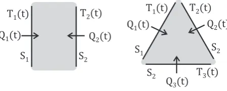
The heat conduction problem in this context is defined by Fourier’s equation with constant thermal properties and mixed boundary conditions at a number of surfaces of a non-homogenous solid body. The boundaries and solid domain of the conceptual model are illustrated in Fig. 1. The problem is defined by the following equation and set ofN boundary conditions with constant surface heat transfer coefficients,

∇ ·(λ∇T) =ρC·∂T

∂t (1)

hi·

Ti(t)−T|Si

=λ·∂T

∂n, [i=1 . . .N]

In this form of conduction problem, the primary interest is in the relationship between boundary fluxes and temperatures rather than internal body temperatures. Once the differen-tial equation has been solved to find the temperatures, the boundary heat fluxes of interest can be calculated simply us-ing,

Q_i(t) =S_i·h_i·T_i(t)−T|_Si (2)

the current state to be expressed entirely in terms of current and past temperatures. This principle, and the fact that the linearity of the problem allows the principle of superposition to be applied, is the basis of the discrete response factor meth-ods applied in many building heat transfer programs as well as the DTN approach described here.

Q (t)2

Q (t)2

Q (t)1

Q (t)1

Q (t)3

S2

S2

S2

S2

S1

S1

T (t)1

T (t)1

T (t)2

T (t)2

T (t)3

Figure 1: Two and three-surface solid body domains and surfaces at which boundary conditions are applied.

The principle advantages of the DTN approach to calcu-lating transient conduction heat transfer, when compared to other response factor methods, can be summarized as fol-lows:

• arbitrary three-dimensional shapes can be treated;

• three or more surfaces with their own boundary condi-tions can be defined;

• exact discrete forms for piecewize linear boundary con-ditions can be derived;

• a wide range of analytical or numerical models can be used to derive the required response factors;

• transient simulation using this method is considerably more efficient than numerical approaches such as tran-sient finite element or finite difference models.

The method is also computationally robust and can deal with thermally massive structures. It is also possible to model con-structions with internal heat sources, such as radiant slabs, by defining one of the surfaces as an internal cylinder. Al-though the calculation of the required response factors can take some effort for a three-dimensional problem, once the values are found they can be stored for later use in simula-tions.

In this paper we provide an outline of the DTN method and present a numerical approach to the calculation of the required discrete weighting factors. The weighting functions and their discrete counterparts employed in the DTN method can be found from calculation of surface heat fluxes when the construction or solid body of interest is excited by com-binations of steps in boundary temperature. The method used to make these step response calculations may vary. Our primary interest has been in applying the DTN method to two and three-dimensional ground heat transfer problems

[6]and so we have developed a numerical method to calcu-late step response fluxes. We propose this is used in simple

multi-layer wall problems (i.e., one-dimensional heat trans-fer) as well as multi-dimensional geometries. The accuracy of the method is examined here firstly with reference to ana-lytical solutions for plane walls. The accuracy of the underly-ing numerical model is furthermore verified with reference to analytical three-dimensional ground heat exchange solution and an example ground heat transfer simulation is presented to demonstrate the computational efficiency of this approach. The step responses used to derive the discrete weighting factors used in the DTN approach can result in very long data series. The sequences of weighting factors required for the DTN calculations can be small for two-dimensional building fabric models. However, for more complex thermally mas-sive constructions the sequences can be very long, as can the temperature histories that have to be continually updated. To make the computation more efficient, and the input data more manageable, Wentzel[5]proposed a weighting factor reduction strategy to reduce the quantities of input data. In this work we have tested this approach but also show how it may be improved for thermally massive structures like base-ments and ground heat exchangers. In this way, the volume of data becomes more manageable, and integration with sim-ulation tools more feasible.

One of the features of the DTN formulation is that bound-ary conditions are defined by constant heat transfer coeffi-cients. This is potentially disadvantageous in building heat transfer problems where the boundary conditions may be non-linear, for example by virtue of radiant exchange. We show how more complex boundary conditions can be accommo-dated.

2. Response factor methods

The various response factor methods that have been de-veloped and applied to building heat transfer problems, and the techniques used to calculate the discrete factors, differ according to:

(i) the form of excitation used to generate the response factors (step, ramp or triangular);

(ii) the computational effort required to generate the re-sponse factor data;

(iii) the length of the response factor data series; (iv) the robustness of the data generation procedures;

(v) the accuracy of the final temperature and heat flux cal-culations;

(vi) whether thermally massive elements can be dealt with; (vii) whether multi-dimensional problems can be treated

Useful reviews of response factor methods can be found in

[8]and[9]but it is worth commenting on some key features in relation to the DTN method discussed here.

Nomenclature

C specific heat capacity, kJ kg−1K−1

h heat transfer coefficient, W m−2K

K conductance, W K−1

¯

K modified conductance, W K−1

L layer thickness, m

n surface normal

N number of surfaces

P period, s

q aggregation level

Q heat transfer rate, W

¯

Q average heat transfer rate, W

r pipe radius, m

S surface area, m2

t time, s

∆_{t time step size, s}

T temperature, °C

¯

T weighted average temperature, °C

∆_{x cell size, m}

Greek symbols

α thermal diffusivity, m2s−1

ω,ϕ,ψ time step, s

κ weighting function

λ thermal conductivity, W m−1K−1

ρ density, kg m−3

τ time (integration variable), s

θ hourly time variable, h

Θ _{daily time variable, days}

Subscripts c cell

i,j surface number

n time step index

a admittive

t transmittive

ρ weighting factor index

response factors. Mitalas and Stephenson[12]made impor-tant improvements by using an analytical model of a multi-layer wall and triangular pulse excitation. In a further de-velopment of this work[13]using a z-transform method and a triangular form of pulse excitation was demonstrated to result in relatively short response factor series when flux his-tory terms were introduced. This Conduction Transfer Func-tion (CTF) formulaFunc-tion includes the current and past tem-peratures on each surface and the past heat flux history on the respective opposite surface. The equations for the inner and outer surfaces are consequently coupled and have to be solved simultaneously. This approach was adopted in a num-ber of building simulation tools[14–17]and remains popu-lar.

The nature of all response factor methods is that, although the calculation required at each simulation time step is rela-tively simple, a much greater computational effort is required to derive the response factors. Essentially three approaches have been taken to deriving CTF data and these differ in their robustness, computational burden and accuracy[18]. These approaches can be classed as Frequency Domain[9, 21, 22], Time Domain[23–27]and State-space[28–30]formulations. The original frequency domain approach was to use Laplace transforms for multi-layer constructions and search for the roots of the hyperbolic characteristic function using a ’direct root-finding method’. This process is not always robust and can result in errors if all the roots are not found. Improved root finding methods have been developed[19, 20]but diffi-culties remain if the time step size is small or the construction has high thermal mass.

The state-space approach avoids the problems of root find-ing but some discretization error is introduced by the reliance on an underlying finite difference formulation using a limited number of nodes. The robustness and accuracy of a number of these approaches to coefficient calculation were tested by Li et al. [18]and significant errors were found in results for structures with high thermal mass when using both Direct Root Finding and State Space calculation methods.

An important advantage of the State Space approach is that, provided a suitable finite difference mesh can be de-fined, the method can be applied to two and three-dimensional constructions [32]. However, because of the matrix inver-sions and integrations required in this approach, dealing with three-dimensional meshes becomes particularly burdensome. Attempts have been made to adapt the CTF approach to the modelling of multi-dimensional problems by trying to derive equivalent multi-layer constructions that approximate the re-sponse of the three-dimensional form[33, 34]but this has re-quired rather heuristic adaptation of the response factor data and consequently makes the calculations difficult to general-ize and automate.

of weighting factors to a manageable finite set of data. The significance of these potential errors is discussed later in this paper.

3. An outline of the Dynamic Thermal Network method

The DTN approach to the analysis of transient conduction is not widely known at present and so we present an overview of the theory here. Details of the development of the method, along with proofs of the essential mathematical principles, can be found in the report by Claesson [3]and also in the thesis by Wentzel[5]. Example applications have also been reported in some conference papers[1, 2, 4, 35–37]

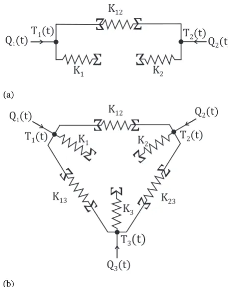
The DTN method has been conceived, as the name sug-gests, as an extension of the network concept often used in the analysis of steady-state conduction heat transfer prob-lems. In such networks, nodes represent points or surfaces with a defined temperature and connections between nodes with finite conductances represent heat transfer paths. One of the essential features of the DTN method is that heat fluxes at each surface are separated into admittive (or absorptive) and transmittive components. This is reflected in the network model in that a single ended heat transfer path is associated with each surface node to represent the admittive heat trans-fer path. Representations of the two and three-surface bod-ies illustrated in Fig. 1 are shown in dynamic network form in Fig. 2. In principle a DTN may incorporate any number of surfaces between which there are conductive heat trans-fer paths. The surfaces can be arbitrary in form and can also be groups of surfaces to which the same boundary condition applies.

The dynamic form of thermal network (Fig. 2) includes constant conductances in a similar manner to the steady-state form. The reversed summation symbols (Σ_{) adjacent these} conductances indicate that the driving temperatures are aver-ages of the current and previous temperatures. In the single ended admittive path the single summation sign indicates the driving temperature is a function of the average temperature at that boundary alone.

The temperatures (Ti(t)) and fluxes (Qi(t)) of the dy-namic network are defined at environmental temperature nodes rather than at the surfaces themselves—the boundary condi-tions in Eq. (1) being of the mixed type—and we make a dis-tinction between the terms boundary and surface in the fol-lowing discussion. The conductances in the admittive path (shown with a single subscript Ki) are equal to the surface area multiplied by a constant heat transfer coefficient, e.g.,

K1=S1·h1. There are constant conductances between each

pair of surfaces (shown with double subscriptsK_{i j}) that de-fine the resistance along the transmittive path. These con-ductances are the overall steady-state concon-ductances between the boundaries and include the surface conductancesK_iand

K_j.

The nodal heat balance equations set out the relationship between the total flux at each boundary and the admittive and transmittive components. For a two and three-surface

Ó

Q (t)

Q (t)

K

K

K

T (t)

_{T (t)}

2

Ó

Ó

Ó

(a)

Ó

Ó

Ó

Ó

Ó

Ó

Ó

Ó

Ó

Q (t)

Q (t)

Q (t)

K

K

K

K

K

K

T (t)

T (t)

T

(t)

(b)

Figure 2: Dynamic Thermal Network representations of a two (a) and three-surface problem (b). The sigma symbols indicate driving temperatures that are weighted averages.

problems the heat balance equations are respectively,

Q₁(t) =Q_1a(t) +Q₁₂(t)

Q2(t) =Q2a(t) +Q21(t) (3)

and,

Q₁(t) =Q_1a(t) +Q₁₂(t) +Q₁₃(t)

Q2(t) =Q2a(t) +Q21(t) +Q23(t)

Q₃(t) =Q_3a(t) +Q₃₁(t) +Q₃₂(t) (4)

The transmittive fluxesQi j(t)are from surfaceitowards sur-face j as indicated by the ordering of the subscripts. More generally, for a network ofN surfaces, there areNheat bal-ance equations with one admittive term in each and(N−1) transmittive terms:

Qi(t) =Qia(t) +Qi j(t) +. . .+QiN(t)

[i=1 . . .N,j=1 . . .N,i6=j] (5)

Q (ô)₁

Q (ô)_1a

Q (ô)₁₂

Time (ô)

K₁₂

K₁

Heat transfer rate

(a)

Q (ô)₁

Q (ô)_1a

Q (ô)₁₃

Q (ô)₁₂

Time (ô)

Q (ô) + Q (ô)_{12 13}

K₁₂

K_{12 13}+ K

K₁

Heat transfer rate

(b)

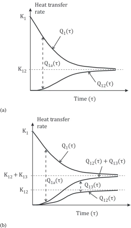
Figure 3: Heat flux responses characteristic of unit step-changes in bound-ary temperatures for a two (a) and three-surface problem (b). Initial fluxes are limited by the surface conductances and steady-state fluxes by the trans-mittive conductances.

surface conductance. As steady-state is approached the ad-mittive component approaches zero and the transad-mittive flux approaches the steady-state value. At any time, the admittive component is given by the difference between the total sur-face flux and the sum of the transmittive fluxes at the other surfaces.

Claesson[3]showed that the temperature differences driv-ing the absorptive and transmittive fluxes can be defined in an exact manner by the current and weighted averages of the boundary temperatures. The absorptive and transmittive fluxes at a given boundary can be written in terms of the con-ductances and these temperatures as follows,

Qia(t) =Ki· 

T_i(t)− ∞ Z

0

κ_ia(τ)·Ti(t−τ)dτ 

 (6)

Qi j(t) =Ki j· ∞ Z

0

κi j(τ)·

Ti(t−τ)−Tj(t−τ)

dτ (7)

These weighted average temperatures are those associated with the points in the network indicated by a reversed sum-mation symbol (Fig. 2). The temperatures are averaged ac-cording to weighting functions,κ_iaandκ_{i j} for the admittive flux at the surface and the transmittive flux between surfaces respectively. These weighting functions are always positive valued and when integrated in the interval[0,∞]have uni-tary value so that,

∞ Z

0

κ_ia(τ)dτ= ∞ Z

0

κ_{i j}(τ)dτ=1 (8)

A shorthand notation is used to denote these weighted aver-age temperatures as follows,

¯

T_ia(t) = ∞ Z

0

κ_ia(τ)·T_i(t−τ)dτ (9)

¯

Ti j(t) = ∞ Z

0

κ_{i j}(τ)·Ti(t−τ)dτ (10)

Using this notation and substituting Eqs. (6) and (7) into Eq. (5) allows the heat balance equations for each surface to be expressed as,

Q_i(t) =K_i·T_i(t)−T¯_i(t)+ N X

j=1

K_{i j}·T¯_{i j}−T¯_ji

[i=1 . . .N,j=1 . . .N,i6=j] (11)

The dynamic relations between boundary heat fluxes and temperatures for a two-surface problems is then simply,

Q1(t) =K1·

T1(t)−T¯1a(t)

+K12·

¯

T12(t)−T¯21(t)

Q2(t) =K2·

T2(t)−T¯2a(t)

+K12·

¯

T21(t)−T¯12(t)

(12)

As the steady-state is approached each average temperature approaches the related boundary temperature and the admit-tive fluxes become zero. It can be seen that, in the steady-state Eq. (12) reduces to the usual expression for flux in terms

of overall conductance and boundary temperatures (Q₁ =

K₁₂·[T₁−T₂], etc.).

3.1. Step responses

zero and repeating this for each surface (as in Fig. 3). Claes-son showed, by superimposing responses [3], that the re-sponse to the unit step boundary conditions for a two-surface problem has the following mathematically exact form:

Q1(t) =K1·T1(t) +

Z∞

0

dQ_1a

dτ ·T1(t−τ)dτ

+

Z ∞

0

dQ12

dτ ·[T1(t−τ)−T2(t−τ)]dτ (13)

Q2(t) =K2·T2(t) +

Z∞

0

dQ2a

dτ ·T2(t−τ)dτ

+

Z ∞

0

dQ₁₂

dτ ·[T2(t−τ)−T1(t−τ)]dτ (14)

If the integral terms of this equation are compared with Eqs. (6) and (7) it can be seen that the weighting functions can be related to the gradient of the step response fluxes in the following way (the extension to three or more surfaces is straightforward).

κ_1a(τ) =−1

K₁ ·

dQ1a(τ)

dτ

κ2a(τ) = −1

K2

·dQ2a(τ)

dτ

κ₁₂(τ) = 1

K12

·dQ12(τ)

dτ (15)

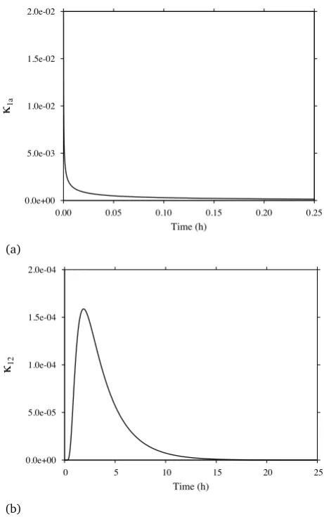
The form of the weighting functions is illustrated in Fig. 4. The admittive weighting function has its maximum value at time zero and decreases rapidly. The transmittive weighting function is initially zero and rises to a maximum after a short time and then tailing off to zero over an extended period. Note that, because the transmittive (cross) fluxes are sym-metric, so are the weighting functions (e.g.,κ₁₂=κ₂₁) and this reduces the total number of weighting factor calculations required.

3.2. Discretization

Claesson[3, 4]showed that the calculation method could be expressed in discrete form, in an exact way, for piecewise linear variations in boundary conditions. When the boundary temperatures are defined by a discrete time series, the aver-age temperatures are calculated by the summation of weight-ing factor sequences multiplied by boundary temperature se-quences that represent the state at previous time steps.The discrete form of Eqs. (9) and (10) is, for current time stepn,

¯

T_ia,n= ∞ X

ρ=1

κ_ia,ρ·Ti,n−ρ (16)

¯

T_{i j,n}= ∞ X

ρ=0

κ_{i j,}ρ·Ti,n−ρ (17)

Where the boundary temperatures vary in a piecewise linear fashion, the weighting factors can be obtained using the ad-mittive and transad-mittive fluxes averaged over each step (size

0.0e+00 5.0e-03 1.0e-02 1.5e-02 2.0e-02

0.00 0.05 0.10 0.15 0.20 0.25

£1a

Time (h)

(a)

0.0e+00 5.0e-05 1.0e-04 1.5e-04 2.0e-04

0 5 10 15 20 25

£12

Time (h)

(b)

Figure 4: Examples of admittive (a) and transmittive (b) weighting func-tions. These represent a single layer concrete wall 100 mm thick.

∆_{t). The discrete weighting factors are then obtained from} the differences in these average time step fluxes as follows,

κ_ia,ρ=Q¯ia(ϕ)−Q¯ia(ω) ¯

Ki

κ_{i j,}ρ= ¯

Qi j(ω)−Q¯i j(ϕ)

Ki j

(18)

where the time differences are betweenϕ= (ρ∆_t−∆_t)and ω=ρ∆_t.

problem (Eq. (12)) can be written as follows,

Q1,n=K¯1·[T1,n− ρs

X

ρ=1

κ_1a,ρT1,n−ρ]

+K12·

ρs

X

ρ=0

κ12,ρ(T1,n−ρ−T2,n−ρ) (19)

Q2,n=K¯2·[T2,n− ρs

X

ρ=1

κ_2a,ρT2,n−ρ]

+K₁₂· ρs

X

ρ=0

κ_12,ρ(T_2,n−ρ−T1,n−ρ) (20)

Using a step-response calculation to find the weighting factors has some advantages compared to methods that use triangular excitation. Firstly, the calculation is independent of any time step size. In principle, once the response is cal-culated, weighting factor data for any choice of time step can be derived. Secondly, it is possible to calculate and process the step response data to a higher level of accuracy and more robustly than triangular pulse data and where root finding procedures are required. Furthermore, employing a step re-sponse without restricting the duration of the excitation al-lows thermally massive structures to be correctly represented. It is worth noting that, as the summation of the transmit-tive weighting factors starts at index zero, this implies that the current temperature at other surfaces is required to find the flux at the surface of interest. In some simulations this temperature may not be known and so iteration may be re-quired. (This is generally the case in building heat balance calculations using the CTF approach.) However, in the DTN method it is generally the case that the first coefficient of the transmittive weighting factor series is insignificant or often zero (see Fig. 4). Consequently, it is often accurate to start the summation of the transmittive weighting factor and tem-perature products starting at indexρ=1 in Eqs. (19) and (20). This may simplify the simulation procedure and avoid iteration in many cases. This feature of the DTN formulation arises from the fact that admittive and transmittive fluxes are treated separately.

4. Boundary conditions

The DTN is formulated, and the step response data cal-culated, assuming that surface heat transfer coefficients (h) are constant. This assumption may suffice for some prob-lems but is potentially limiting as there are many situations where boundary conditions are more complex, for example, by virtue of radiation or mass transfer being in effect at the surface, or where there is a dependance on thermal proper-ties that are functions of temperature. Treatment of radiant heat exchange boundary conditions has been commented on by Kalagasidis[37]. The general approach we have taken to work around this assumption has been to define a boundary temperature that is an ’effective temperature’ (T_e) that, when

1 2 3 4 5 6 7 8 9 10

10

8

6

4

3

0

Q (ô)1a

Q (ô)_1a K₁

Q (0) = ₁ K₁

H

e

a

t

T

ra

n

sf

e

r

R

a

te

(

W

)

Time (hours)

(a)

31 32 33 34 35 36 37 38 39 40

10 x 10-4

6

4

0

Q (ô)₁₂

Q (31h)₁₂

Q (ô)₁₂

H

e

a

t

T

ra

n

sf

e

r

R

a

te

(

W

)

Time (hours)

(b)

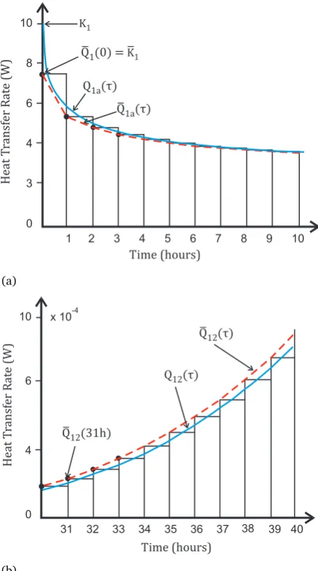
Figure 5: Step-response for (a) admittive, and (b) transmittive fluxes (solid lines). Flux averages are shown as dotted lines, with bars representing the average value over each time step.

applied using the predefined constant heat transfer coeffi-cient, gives the expected surface heat flux as applying a more complex boundary condition model. This effective temper-ature (or environmental tempertemper-ature) does not correspond directly to a physical boundary temperature but is applied in the DTN heat balance equations and when the weighted av-erage temperature is updated. This approach is one that can be generalized. Two particular types of boundary condition have been tested[6]that illustrate this concept: at external surfaces and at pipe surfaces.

4.1. External surface boundary conditions

boundary condition is,

Qi

Si

=R_sw+R_{l w}+h_ca(T_a−T_Si) (21)

The effective boundary temperature is intended to give the equivalent heat flux and hence is defined by,

Q_i

S_i =hi(Te−TSi) (22)

Hence the equivalent or environmental temperature must be,

Te= [Rsw+Rl w+hcaTa+ (hca−hi)TSi]/hi (23)

This expression involves the surface temperature and so im-plies that some iteration may be required to calculate Te. If the surface convection coefficient is constant and the same as that assumed in the DTN model, then the term involving the surface temperature is zero. In that case the effective temperature follows the usual definition of sol-air tempera-ture: T_e = T_a+ (R_sw+R_{l w})/h_i. If the surface temperature changes slowly relative to the time step—as it does in many building and ground heat transfer problems—then the sur-face temperature calculated at the previous time step can be used in the last term of Eq. (23) with little error and iteration avoided.

4.2. Pipe surface boundary conditions

In geometries with embedded or buried pipes such as ra-diant floor heating systems or horizontal ground heat ex-changers, the heat flux at the pipe surface is a significant driver of the network heat balance. The pipe surface can be readily incorporated into a three-surface DTN representation but the boundary condition requires further consideration. In particular, it is usually necessary to define the relationship between the boundary temperature and both the pipe fluid inlet and outlet temperatures. Our approach is—similar to that of Strand[32]—to assume the pipe surface temperature does not vary along its length and make an analogy with an evaporating-condensing heat exchanger and so to define a characteristic effectiveness parameter. The pipe fluid heat balance is then defined by the maximum possible tempera-ture difference and the effectiveness as follows,

Q_p(t) =ǫmC T˙ _in(t)−T_p(t) (24)

For such a heat exchangerǫ=1−e−N T U_{and this is related to} the total pipe area and fluid heat transfer coefficient by the Number of Transfer Units (NTU) according to,

N T U=2πr H.hp ˙

mC (25)

The relationship between the pipe surface temperature and the boundary temperature (T_i(t)) that needs to be found for use in the DTN heat balance equations, is defined (as in Eq.(2)) by the surface heat flux relationship,

Qi(t) =hi.Si Ti(t)−Tp(t)

(26)

In an iterative procedure, the boundary temperature (T_i) is initially estimated and the boundary flux is found from the pipe surface heat balance, Eq. 26. The boundary temperature value is refined using Eq. 24 to find an estimate of the pipe surface temperature (TP). The revised estimate of the bound-ary temperature is successively substituted into the boundbound-ary temperature heat balance until the overall heat transfer rate is consistent with the calculated boundary flux. The outlet temperature can then be found from the fluid heat balance:

Tout(t) =Tin(t)−QP(t)/mC˙ .

It is necessary to apply an adiabatic condition to the pipe surface when the flow rate becomes zero. This can be done by setting the flux to zero and solving for the boundary tem-perature. Although this temperature is not of direct interest when the flow rate is zero, it is necessary to find the value and use it to update the average temperature during the progress of the simulation. This approach to the treatment of pipe boundary conditions was tested and validated in a ground heat exchanger application reported in[6].

5. Weighting factor reduction

Both the weighting factor data series and the temperature histories that need to be stored and processed can, in prin-ciple, be very long. More than one thousand factors may be need to be integrated before the steady-state is approached with sufficient accuracy—depending on the thermal proper-ties and scale of the construction. In addition to increasing the data storage requirements, updating the long tempera-ture histories can be time consuming so that there may be no advantage over conventional numerical methods. To make the computation more efficient, a weighting-factor reduction strategy that aggregates later values and that was developed by Wentzel[5]has been implemented.

In this approach, the weighting factor series is divided into several sub-series (levels) that have increasing time step size. The procedure is slightly different for the admittive and transmittive components. For the transmittive weighting fac-tors (κ12 , etc.) the initial interval of (∆t) is used as the

time step (aggregation interval) until the series reaches the maximum value. After the weighting factors decrease below half of the maximum value (κma x/21) the step size is doubled and the weighting factors aggregated accordingly. The sec-ond level (q=2) starts after the values have halved again, i.e. κ_{ma x}/22and the time step length becomes 2∆_t. Simi-larly, the third level (q=3) starts after the values have de-creased below one-fourth of the maximum until they below one-eighth of the maximum value, κ_{ma x}/23_{, and the time}

and their reduced or aggregated form are shown in Figs. 6 and 7.

0 0.02 0.04 0.06 0.08 0.1 0.12 0.14

10 20 30 40 50 60 70 80 90 100 £1a

Time (h)

(a)

0 0.02 0.04 0.06 0.08 0.1 0.12 0.14

10 20 30 40 50 60 70 80 90 100 £1a

Time (h)

level q=1

level q=2 level q=3

level q=4

(b)

Figure 6: Discrete admittive weighting factor values and the corresponding reduced set. This shows the first 100 hours from a series with a time step size of 1 hour.

Aggregating the response data and temperature histories in this way can potentially introduce errors to the calcula-tions. As temperature data is shifted back in time the aver-aging process at each change in step size (aggregation level) tends to introduce dispersion errors. Wentzel describes an updating procedure that staggers the boundaries between the aggregation levels at alternate time steps that minimizes such problems. In the few test cases reported[5]the error asso-ciated with the data reduction process was demonstrated to be less than 0.3%.

5.1. An improved weighting factor reduction strategy

The reduction strategy proposed by Wentzel[5] aggre-gates the transmittive weighting factors by doubling the time step size included after the factors have decayed to half of the previous value. Several ’levels’ (q) with increasing time step sizes are created as a result of the reduction process. This may often reduce the weighting factors required by two or-ders of magnitude and for structures such as plain walls the

0 0.01 0.02 0.03 0.04 0.05 0.06

10 20 30 40 50 60 70 80 90 100

£12

Time (h)

(a)

0 0.01 0.02 0.03 0.04 0.05 0.06

10 20 30 40 50 60 70 80 90 100

£12

Time (h)

level q=1 level q=2

level q=3

level q=4

(b)

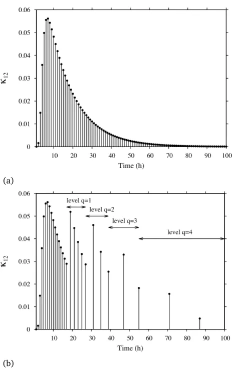
Figure 7: Discrete transmittive weighting factor values and the correspond-ing reduced set. This shows the first 100 hours from a series with a time step size of 1 hour.

number of factors is modest. In a study of ground heat ex-change around basement structures[6]the authors found the history needed to be extended to several decades to fully cap-ture the behaviour of the system. In this study a horizontal ground heat exchanger and basement structure were mod-elled. A three-surface DTN network was used where surface 1 represented the inside basement and floor surfaces, surface 2 represented the horizontal ground surface and surface 3 rep-resented the collective heat exchanger pipe surfaces. This is illustrated in Fig. 8.

Figure 8: A horizontal ground heat exchanger and basement structure mod-elled using a three-surface DTN

In order to improve this situation a more aggressive re-duction process has been implemented. In this procedure the number of weighting factors at each level of reduction is strictly limited. After a certain number of factors at a given level have been calculated the time step is forced to double. This occurs independently of whether the weighting factor values have fallen to half of the previous value. A range of parameter values controlling the initial level, tolerances and number of factors per level have been tested [6]. Good re-sults have been obtained when limiting the number of admit-tive and transmitadmit-tive weighting factors per level to 5.

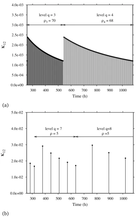
The application of the proposed reduction method is illus-trated in Fig. 9 where the transmittive response factors over two levels of reduction are compared with those calculated using Wentzel’s approach. It can be seen that, in this exam-ple, at the third level of reduction 70 weighting factors would be replaced by 5 using the proposed aggressive method. In the proposed method the transition from one level to the next tends to occur earlier than the original method and so the time period shown in Fig. 9 is spanned by levels 7 and 8 in our aggressive reduction approach as opposed to levels 3 and 4.

The length of the weighting factor series in the complete form, Wentzel and more aggressive reduction methods are compared in Table 1 for the ground heat exchanger geometry illustrated in Fig. 8. In this case it was found that the admit-tive weighting factor weighting seriesκ_1aandκ_2a could not be reduced below 179 and 221 values respectively without compromising the calculation of the short term responses. The acceptability of the reduction was judged by compar-ing the DTN simulation results with those of the native nu-merical method using the same mesh and boundary condi-tions. There was slightly greater scope for reduction of the transmutative weighting factor data series in this case. Ta-ble 1 also highlights the significant increase in computational speed that results from the reduction in the length of the weighting factor series.

0.0e+00 5.0e-04 1.0e-03 1.5e-03 2.0e-03 2.5e-03 3.0e-03 3.5e-03 4.0e-03

300 400 500 600 700 800 900 1000

£12

Time (h)

level q = 3 ₃ = 70

level q = 4 ₄ = 68

(a)

0.0e+00 1.0e-02 2.0e-02 3.0e-02 4.0e-02 5.0e-02

300 400 500 600 700 800 900 1000

£12

Time (h)

level q = 7 = 5

level q=8 =5

(b)

Figure 9: Discrete transmittive weighting factor series reduced using the Wentzel’s method (a) and the proposed more aggressive reduction method (b). This particular example shows the hours corresponding to the third and fourth levels of the Wentzel method.

Our enhanced reduction approach was demonstrated to improve the computational speed by more than three orders of magnitude compared to the full data series (no reduction) and nearly two orders of magnitude compared to Wentzel’s original approach. Whether this more aggressive approach is necessary seems dependent on the nature of the latter part of the transmittive weighting function. In the case of the basement geometry the tail of the function was rather linear and so the original approach (waiting until the values fell by a factor of two before incrementing the aggregation level) was not effective. In the case of plane wall geometries the original approach seems to reduce the data to a practical level.

6. Numerical methods

Reduction method None Wentzel Agressive

Total number ofκ_1a 105 _{61,812 179}

Total number ofκ_2a 105 _{70,211 221}

Total number ofκ_3a 105 _{77 71}

Total number ofκ12 105 34,145 76

Total number ofκ13 105 46,758 78

Total number ofκ23 105 9,571 87

Time to complete 7.6 h 29 min 4.47 s

Table 1: A comparison of the quantity of weighting factors according to re-duction procedure along with the corresponding time to complete an annual simulation.

may vary. For simple plane multi-layer walls analytical so-lutions can be used to achieve high accuracy [38]but for multi-dimensional shapes analytical approaches are seldom tractable. Wentzel [5]used a numerical method to derive fluxes for a basement and whole house geometry. The nu-merical model was applied with a fixed one hour time step. The difficulty in using a numerical model in this way is that firstly, the initial absorptive fluxes will not be captured ac-curately as these occur over relatively short timescales and secondly, to capture the long timescale transmittive flux com-ponents would require an excessive number of hourly time steps.

The approach taken to overcome these difficulties was to combine the numerical results with those from different ana-lytical solutions for short and long timescales. An anaana-lytical solution for short timescales was adopted and blended with the numerical results without particular difficulty. Blending a solution for the longest timescales was shown to be possible but required some user expertise in the choice of model and interpolation coefficients. A more automated and general-ized approach is required if the DTN method is to be applied in practical simulation tools. To this end, we have developed an entirely numerical approach.

Our primary interest has been in applying the DTN method to two and three-dimensional ground heat transfer problems

[6] and so we have developed a numerical method to cal-culate step response fluxes that is capable of dealing with complex geometries and spatially varying thermal proper-ties. To address the challenges of accurately capturing the ini-tial absorptive fluxes and efficiently calculate long timescale fluxes, particular spatial and temporal discretization proce-dures have been found necessary and are described below. The numerical method and subsequent DTN calculations have been verified by reference to two different analytical solu-tions.

6.1. Numerical conduction model

We have used an implementation of the Finite Volume Method in the form of the code known as the General Ellip-tical Multi-block Solver (GEMS3D) to generate the required step-response flux histories. The solver applies the Finite Vol-ume Method to solve the general convection-diffusion

equa-tion on three dimensional boundary fitted grids. The numer-ical method is similar to that described for complex geome-tries in Ferziger and Peric[39]and is described in some de-tail by He[40]. The GEMS3D solver has been used to model ground heat exchanger problems in a number of projects (e.g.,

[41]). Model verification and validation of this solver has also been reported elsewhere by Young[42]. The sets of alge-braic equations arising from the discretization on the multi-block mesh are solved using an iterative method based on the Strongly Implicit Procedure[43]adapted to allow communi-cation of data across block boundaries during the iterative procedure. Using a block-structured approach also allows a degree of parallel processing by the solving the equations of each block with separate threads.

To develop a numerical procedure suitable for efficient calculation of the step response data, we have implemented a variable time-stepping feature in the GEMS3D solver. This allows the calculation of the admittive flux with very small time steps (of order 0.01 seconds) and the time step size to be gradually increased in a geometric fashion so that the last time steps (approaching steady-state) may be a number of months. To achieve the variable time stepping in an accurate and numerically stable manner, a second order backwards differencing scheme has been adopted. The formulation by Singh and Bhadauria allows steps of varying size but retains second order accuracy[44]. For the current time step size, ∆_tn_{and previous time step size,}∆_tn−1_{, the temporal} differ-ential is approximated according to,

∂T

∂t ≃

2∆_tn₊∆_tn−1 ∆_tn₍∆_tn₊∆_tn−1₎T

n₊∆tn+∆tn−1 ∆_t∆_tn−1 T

n−1

− ∆t

n

∆_tn−1₍∆_tn₊∆_tn−1₎T

n−2 ₍₂₇₎

whereTn−1 _andTn−2 _{are the temperatures at the two}

pre-vious time steps. In the case of thermally massive structures increasing the time step allows the total number of steps re-quired to be reduced by at least two orders of magnitude compared to using one that is fixed. At the same time, very small time steps at the start of the step response calculation can be accommodated. The need for such small time steps in order to accurately calculate the initial heat flux is high-lighted in the discussion of verification tests below.

6.2. Mesh generation

generation of the mesh for the ground heat exchanger ge-ometry shown in Fig. 8 in which case the mesh is defined by parameters such as pipe spacing, basement depth. Examples of parametric variations in mesh geometry and configuration are illustrated in Fig. 10. A similar parametric approach can be taken for geometries such as framed walls and floors with embedded pipes.

Figure 10: Parametric variations in ground heat exchanger mesh geometry and pipe configuration. Principle block boundaries are highlighted on one face. The colours indicate regions with different thermal properties. The base configuration is illustrated in Fig. 8.

7. Verification exercises

The proposed approach to numerical implementation of the DTN method has been verified and accuracy evaluated in the following exercises: (i) comparison of the numerical model and analytical step response calculations; (ii) compar-ison of the numerical model and DTN results with analytical model results for multi-layer walls under periodic excitation.

7.1. Numerical calculation of step responses

As the primary objective of employing a numerical method-ology is to derive the required step response data, it is partic-ularly useful to make comparisons between numerical predic-tions and those calculated from an analytical model of a step response. A suitable analytical solution for a single-layer wall has been published by Xiao et al.[46]and is employed here. In addition to verifying the underlying numerical model and the solution of the conduction equation for the given bound-ary conditions, the tests also examine the spatial and tempo-ral discretization errors and the practices proposed to limit such errors.

It might be expected that discretization errors are a func-tion of mesh density, temporal discretizafunc-tion and mesh smooth-ness: this has been found to be the case here. Previous work on the application of Finite Difference methods to the mod-elling of conduction in building fabrics is informative with regard to quantifying errors and guidelines for mesh distri-bution. Much of this work[47–49]was concerned with ap-plying course meshes and avoiding conditions of instability in the case of semi-explicit methods. It was shown that er-rors and mesh densities can be characterized according to Fourier Number given by, Fo = α∆_t/L2_{. Although} stabil-ity is not a concern in the proposed method (it being a fully implicit formulation) and dense meshes being more afford-able for a one-off step response calculation, normalisation of time and spatial scales according to Fo is useful. The fea-tures of the step response calculation found to be sensitive to the mesh and the temporal discretization are the initial heat flux and, slightly later in the calculation, the transmitted flux during the period where this changes most rapidly. These timeframes correspond to Fo much less than 1 and around the time corresponding to Fo equal to 1 respectively.

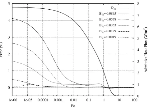
The initial heat flux in the step response calculation is the peak admittive flux and is limited by the surface heat trans-fer coefficient. This condition corresponds to a steep temper-ature gradient immediately adjacent the surface. Capturing this initial temperature gradient and peak admittive flux is challenging in a numerical model given the finite cell size at the surface and discrete time steps. It has been found that, to capture this feature with sufficient accuracy requires both a very small initial time step and a small mesh cell size (layer thickness) at the surface. The admittive flux for a 100 mm concrete wall calculated using the analytical solution[46]is shown in Fig. 11 along with the errors between this solution and numerical results using different meshes

0 1 2 3 4 5

1e-06 1e-05 0.0001 0.001 0.01 0.1 1 10 100

0 1 2 3 4 5 6 7 8

E

rror (%)

A

dm

it

ti

ve

H

e

a

t F

lux (W

/m

2)

Fo

Q1a

Bi_c= 0.0895

Bi_c= 0.0578

Bi_c= 0.0353

Bic= 0.0129

Bic= 0.0019

Figure 11: Error in admittive flux calculated for a plane wall with different mesh distributions. Meshes are characterized according to the Biot Number of the cells next to the surface. The solid line, plotted against the righthand axis, indicates the admittive heat transfer rate according to the analytical solution.

to vary with Bi_C in a very linear manner. This demonstrates that the error in the initial flux prediction can be reduced to a very small value by controlling the cell size at the surface.

0.0e+00 1.0e-02 2.0e-02 3.0e-02 4.0e-02 5.0e-02

0 0.02 0.04 0.06 0.08 0.1

Ini

ti

a

l A

dm

it

ti

ve

F

lux E

rror

Bi_c

Mesh data

Error = 0.005 Bi_c

Figure 12: Variation in initial admittive flux error according to surface cell Biot Number.

The cell size in a plane wall is expanded in size from the small value at the surface to a maximum value near the centre of the layer. It has been found that the error in the transmit-tive flux, and hence the peak transmittransmit-tive weighting factor, is dependent both on the order of the temporal discretization and the maximum cell size that occurs at this location. In all cases, the maximum error in transmitted flux (which occurs at a time corresponding to approximately Fo=1) is noticeably reduced by adopting a second order temporal differencing scheme rather than a basic first order Euler method. Hence, we have adopted the second order method given in Eq.27

in the results reported here. (The second order central dif-ferencing scheme is adopted in the case of spatial discretiza-tion.) Errors in transmitted flux using different mesh densi-ties are shown in Fig. 13. In this analysis of the transmittive flux error, a Cell Fourier Number, FoC, has been defined for the cell at the centre of the layer. A timescale can be defined that is a characteristic of the layer and corresponds to the decay time[50].

τin f = (2L)2

π2_α (28)

This timescale, along with the cell size,∆_x

c, can be used to define the Cell Fourier Number according to,

Foc= ατ_{in f}

∆_x2

c

(29)

-1.5 -1 -0.5 0 0.5 1

0.01 0.1 1 10 100

0 0.2 0.4 0.6 0.8 1 1.2 1.4

E

rror (%)

T

ra

ns

m

it

ti

ve

H

e

a

t F

lux (W

/m

2)

Fo Q₁₂

Fo_c = 7.22 Fo_c = 21.9 Fo_c = 44.7 Fo_c = 75.5 Fo_c = 114 Fo_c = 134 Fo_c = 206

Figure 13: Error in transmittive flux calculated for a plane wall with differ-ent mesh distributions. Meshes are characterized according to the Fourier Number of the cells at the centre of the wall. The solid line indicates the transmittive heat transfer rate according to the analytical solution.

The maximum absolute errors in transmittive flux shown in Fig. 13 always occur shortly before the time correspond-ing to Fo=1. This maximum absolute error is plotted against Focin Fig. 14. The error is shown to vary inversely with Foc and closely follows the correlation Error=0.054·Fo−_c1. This demonstrates that the error can be reduced to a reasonably low level by control of the maximum cell size.

These correlations between estimated error and the cell sizes at the surface and centre of the wall layer can serve as a basis for systematically determining mesh parameters in an automated mesh generation procedure. It has been found that, as there can be a significant difference between the cell size at the surface and the larger cell at the centre, it is also important to ensure a smooth transition in cell size to ensure errors at other times during the step response calculation do not exceed those quantified above.

7.2. Periodic excitation of multi-layer walls

0.0e+00 5.0e+02 1.0e+03 1.5e+03 2.0e+03 2.5e+03 3.0e+03 3.5e+03 4.0e+03

0 50 100 150 200 250

T

ra

ns

m

it

ti

ve

F

lux 1 /

E

rror

Fo_c

Mesh data

1/Error = 18.5 Fo_c

Figure 14: Variation in maximum transmittive flux error according to central cell Fourier Number.

weighting factors derived from the numerical model. The dif-ferences between the DTN calculation results and those from an analytical solution reflect potential errors in the underly-ing numerical model (discussed above), the weightunderly-ing factor reduction, as well as the discrete nature of the DTN calcula-tion. In this verification exercise results have been compared with an analytical solution for a multi-layer wall with a con-stant inside temperature and periodic excitation of the out-side air temperature. The analytical solution is reported by Xiao et al. [46]and is based on the method for multi-layer constructions by Pipes [51]. The periodic boundary condi-tion is defined byT₂=T_mean+T_ampsin(2πt/P). The solution gives the periodic variation in heat flux at the inside surface which can be compared withQ₁(t)/A₁ in the DTN calcula-tion.

Two wall constructions are defined in this exercise; one heavyweight and one lightweight. These consist of gypsum or concrete layers alongside a layer of insulation. The ther-mal properties of these materials is shown in Table 2. The heavyweight wall consists of 150 mm of concrete inside and 201 mm of insulation outside. The lightweight wall consists of 13 mm of gypsum inside and 202 mm insulation outside. The convection coefficients, hc, are 7.7 and 25 Wm−2.K at the inside and outside surfaces respectively. In both cases the overall conductance (U-value)K₁₂=0.189 Wm−2_.K.

The inside heat fluxes calculated using the DTN model of the multi-layer wall are compared with both the analytical solution and the numerical model results in Figs.15 and 16 for the concrete and gypsum walls respectively. The upper plot in these figures shows the boundary periodic variation in outside temperature and the characteristic periodic variation in inside flux. In these calculations the period of excitation is 24 hours and the DTN calculation time step is 5 minutes.

Material λ ρ C α

W.m−1_K−1 _kg.m3 _kJ.kg−1_K−1 ₁₀−7_m2_s−1

Concrete 1.7 2300 900 8.21

Gypsum 0.22 900 800 3.06

Insulation 0.04 50 864 9.26

Table 2: Material properties for the walls used in the verification study using periodic boundary conditions.

The mean temperature (Tmean) was 20°C and the amplitude of excitation (Tamp) was 15°C.

0 0.02 0.04 0.06 0.08 0.1

0 12 24 36 48 60 72 84

E

rror (%)

Time (h)

DTN vs Analytical DTN vs Numerical

0.0 10.0 20.0 30.0 40.0 50.0

-1.0 -0.5 0.0 0.5 1.0 1.5

T

em

pe

ra

ture

(

o C)

H

ea

t F

lux (W

/m

2)

External Temperature Inside flux

Figure 15: Differences between DTN, numerical and analytical predictions of wall heat flux under periodic excitation for the heavyweight concrete wall.

As there are acknowledged discretization errors in the re-sults of the numerical conduction calculations, and the dis-crete weighting factors used in the DTN calculation are de-rived from this data, it is to be expected that there is better agreement between the DTN and numerical results than be-tween the DTN and analytical results. This trend is apparent in Figs.15 and 16. The errors show some periodic fluctu-ations such that the greatest errors occur when the flux is changing most quickly. Two sources of error attributable to the DTN calculation are firstly due to the aggregation of the weighting factors. Secondly, some error can be expected as the discrete DTN calculation is only exact for piecewise linear variations in boundary temperature whereas these periodic conditions represent a continuous sinusoidal variation with time. In all these results the error is less than 0.1% and this seems very acceptable—certainly for building heat transfer calculations and energy simulations.

8. Inter-model validation

0 0.02 0.04 0.06 0.08 0.1

0 12 24 36 48 60 72 84

E

rror (%)

Time (h)

DTN vs Analytical DTN vs Numerical

0.0 10.0 20.0 30.0 40.0 50.0

-3.0 -1.5 0.0 1.5 3.0 4.5 6.0

T

em

pe

ra

ture

(

oC)

H

ea

t F

lux (W

/m

2)

External Temperature Inside flux

Figure 16: Differences between DTN, numerical and analytical predictions of wall heat flux under periodic excitation for the lightweight gypsum wall.

tion methods[52]. This set of tests is intended to be used for diagnostic purposes and to allow inter-model comparisons. Tests include a steady-state condition that has a correspond-ing analytical solution and a number of tests of transient heat transfer and annual energy demand calculations for rectan-gular floors directly bearing on the ground. The tests use a range of convective boundary conditions and dimensions. One of these tests in particular (case GC70b) has been used in this work to further verify the DTN calculations, investigate the computational efficiency of the approach, and to allow comparisons with other models.

The geometry in the GC70b test case is simply a 12×12 m square floor area surrounded by an adiabatic wall and a fur-ther 15 m of ground with a ground depth of 15 m. The air temperature adjacent to the floor is constant (30 °C) and the outside temperature (i.e., the surrounding upper ground sur-face temperature) varies according to daily periodic variation superimposed on a seasonal periodic variation. This bound-ary temperature (T2in this two-surface problem) is definied

according to the hourly time variable,θ as follows,

T₂=T_{d a y}−T_{amp,d a y}cos 

2π(θ−4) 24

‹

(30)

and according to a daily time variable,Θ_{, such that,}

Td a y=Tmean−Tamp,seasoncos 

2π(Θ−15) 365

‹

(31)

In this test caseTmean=10 °C,Tamp,d a y=2 °C andTamp,season

= 6 °C. This results in a variation in outdoor temperature from a minimum of 2 °C and maximum of 18 °C over the year and a diurnal variation of 4 °C . The other properties of this test case are summarized in Table 3. This test does not have a known analytical solution but is a simplified rep-resentation of annual building ground heat transfer condi-tions. It is intended that model behaviour is compared in terms of predicted net annual heat transfer (annual heating

demand) in this particular case. A number of sets of test re-sults from a number of heat transfer models and solvers are published in the Annex 43 report [52] to allow such inter-model comparisons. A separate report on the performance of the GEMS3D solver using this test suite has also been pub-lished[53]. Results from a number of numerical models em-ploying fine meshes of the ground geometry are available, along with results from widely used building energy simula-tion tools that generally take simplified approaches to calcu-lating ground heat transfer.

Property Value Units

floor size 12×12 m

wall thickness 0.24 m

domain size 42.24×42.24 m

ground depth 15 m

thermal conductivity 1.9 W.m−1K−1

density 1490 kg.m3

specific heat 1800 kJ kg−1K−1

inside convection coefficient 7.95 Wm−2.K

outside convection coefficient 11.95 Wm−2.K

Table 3: Properties of IEA Annex 43 test case GC70b.

Results for the GC70b test case have been obtained from application of the GEMS3D solver and the corresponding DTN calculations using different levels of weighting factor reduc-tion. The three-dimensional nature of the thermal conditions is illustrated in the visualisation of the ground temperatures predicted by the GEMS3D numerical solver in Fig. 17. The re-sults of this test can be used, firstly, to judge the consistency between the DTN calculation and that of the underlying nu-merical method and secondly, to gain some confidence in the predictions when compared to other models. Here the same mesh (with 3.16×106cells) was used to make the annual cal-culation using the numerical model as used to make the step response calculation and subsequently derive the weighting factors.

The results from the DTN and GEMS3D models are com-pared, in terms of net annual heat transfer, with values re-ported for three well known numerical tools [17, 54, 55]

and three building energy simulation tools [31, 56, 57]in Fig. 18. The results for the DTN method using different forms of weighting factor reduction are shown, along with compu-tation times, in Table 4. Due to the thermally massive nature of this problem it is necessary to simulate a number of years of repeated operation until a steady-periodic state is reached. The computation times in Table 4 are consequently for simu-lation up to the end of the sixth year.

Temperature (C)

4 8 12 16 20 24 28

Figure 17: Temperature distribution around the floor predicted by the GEMS3D numerical model for the GC70b test case at the end of the year (one quarter of the geometry shown). Temperature contours are shown at 2K intervals in the 4–28 °C range.

gives the annual energy, the other numerical methods[17, 54, 55]produce very similar values, ranging from 17.396– 17.552 MWh[52]. The values produced by GEMS3D and the DTN calculations also lie within this narrow band. This jus-tifies a good level of confidence that the values are reason-able and of compatible accuracy to other numerical methods. The results reported for the energy simulation tools are lower and wider ranging. This, in itself, is not surprising in view of the variety of simplified and crudely discretized methods that are employed by these tools in the interests of computational speed.

Method Annual energy Computation time

GEMS3D 17.476 MWh 117 hours

DTN (no reduction) 17.473 MWh 15.1 hours

DTN (Wentzel) 17.475 MWh 18.6 seconds

DTN (aggressive) 17.476 MWh 1.70 seconds

Table 4: Annual energy results and computational times for the GEMS3D numerical model and DTN method using different levels of weighting fac-tor reduction for IEA Annex 43 test case GC70b. Calculation times were recorded on a workstation with a 2.83GHz Xeon processor.

The computation times reported in Table 4 vary signif-icantly. The time required for the numerical model calcu-lations is very long due to the large mesh and the need to simulate several years. Clearly 117 hours is not a practical timescale for regular application to design calculations. The simulation using the DTN approach but with a complete set of weighting factors (106_{in number) is an order of magnitude}

quicker but still too long for practical application. Applying the weighting factor reduction reduces the computation time by more than five orders of magnitude compared to the nu-merical method. The Wentzel reduction method makes the calculation time quite acceptable for repeated applications to

17.476  17.469  17.396  17.434  17.552  16.607 

15.553  16.817 

10  11  12  13  14  15  16  17  18  19  20 

DTN  

GEMS 3D 

TRN SYS 

FLU ENT 

MAT LAB 

SUN REL

Ener gyPl

us  VA11

4 

An

n

u

a

l 

e

n

e

rg

y

 (

MW

h

) 

Figure 18: Annual energy predicted by different models for the IEA Annex 43 test case GC70b. TRNSYS, FLUENT and MATLAB[17, 54, 55]use finite difference or finite element methods. SUNREL, EnergyPlus and VA114[31, 56, 57]are building energy simulation tools that use simplified ground heat transfer methods.

long time series simulations. The more aggressive weighting factor reduction strategy we have applied reduces the calcu-lation time by a further order of magnitude. In this case the effect on computation time of applying the more aggressive reduction method is not as significant as in the simulation of the ground heat exchanger reported above (see Table 1).

It should be noted that, although the computation time for the DTN method with reduced weighting factors is rel-atively short, some consideration has to be given to the ef-fort required to make the preliminary step response calcula-tions. In this case approximately 15 hours was required to make each step response calculation using the dense three-dimensional mesh. The speed advantage of the DTN method in the case of three-dimensional thermally massive structures is apparent when the weighting factors are calculated for a particular geometry and then stored for repeated use in sim-ulation studies over long time series. In the case of structures that are one or two-dimensional in nature, the step response calculation is less burdensome and more practical to carry out at the start of each simulation. In the case of a multi-layer wall all the step response calculations and weighting factor analysis take only a few seconds.

9. Conclusions

The DTN approach to modelling of transient conduction has a number of advantages over other response factor meth-ods. In particular: arbitrary three-dimensional shapes can be treated; three or more surfaces with their own boundary conditions can be defined; exact discrete forms for piecewise linear boundary conditions can be derived; a wide range of analytical or numerical models can be used to derive the re-quired response factors. The numerical procedures are fur-thermore robust and computationally efficient.