This is a repository copy of A new approach to multi-phase formulation for the solidification of alloys.
White Rose Research Online URL for this paper: http://eprints.whiterose.ac.uk/74945/
Article:
Bollada, PC, Jimack, PK and Mullis, AM (2012) A new approach to multi-phase formulation for the solidification of alloys. Physica D-Nonlinear Phenomena, 241 (8). 816 - 829. ISSN 0167-2789
https://doi.org/10.1016/j.physd.2012.01.006
Reuse
Unless indicated otherwise, fulltext items are protected by copyright with all rights reserved. The copyright exception in section 29 of the Copyright, Designs and Patents Act 1988 allows the making of a single copy solely for the purpose of non-commercial research or private study within the limits of fair dealing. The publisher or other rights-holder may allow further reproduction and re-use of this version - refer to the White Rose Research Online record for this item. Where records identify the publisher as the copyright holder, users can verify any specific terms of use on the publisher’s website.
Takedown
If you consider content in White Rose Research Online to be in breach of UK law, please notify us by
A New Approach to Multi-Phase formulation for the
Solidification of Alloys
P. C. Bollada, P.K. Jimack, A. M. Mullis
Institute of Materials Research, University of Leeds, LS2 9JT
Abstract
This paper demonstrates that the standard approach to the modeling of multi-phase field dynamics for the solidification of alloys has three major defects and offers an alternative approach.
The phase field formulation of solidification for alloys with multiple solid phases is formed by relating time derivatives of each variable of the system (e.g. phases and alloy concentration), to the variational derivative of free energy with respect to that variable, in such a way as to ensure positive local entropy production. Contributions to the free energy include the free energy density, which drives the system, and a penalty term for the phase field gradients, which ensures continuity in the variables. The phase field equations are supplemented by a constraint guaranteeing that at any point in space and time the phases sum to unity. How this constraint enters the formulation is the subject of this paper, which postulates and justifies an alternative to current methods.
Keywords:
Multi-phase, Phase field, Lagrange multiplier, Solidification, Crystal growth, Eutectic, Peritectic, Gibbs free energy
1. Introduction
mechanisms behind long-standing problems in solidification such as sponta-neous grain refinement, [8], and predicting the effect of external oscillating fields on dendrites [9]. The key advantage of such models is that by intro-ducing a continuous (differentiable) phase variable, φ, the value of which represents the phase of the material, the need to explicitly track the solid-liquid interface is removed. Instead, the mathematically sharp interface is replaced by a diffuse interface of finite width, the motion of which may be tracked using standard techniques for partial differential equations. Early phase-field models of solidification concentrated on single-phase systems, in which there was the liquid and only a single solid phase present. This gener-ally represented either the thermgener-ally controlled growth of a pure substances (e.g. [10]), or the isothermal solidification of an ideal binary solid-solution [11]. However, the phase-field concept may be extended to systems where there is more than one solid phase present, resulting in multi-phase field mod-els. For a topical review of multi-phase field modelling in material science see [12]. In multi-phase field models the scalar variable, φ, is replaced by a vector, θ, where the ith element θi, is the amount of phase i present1. This
extension has, though, yielded variations in the derivation techniques used to obtain the equations of motion for the interface from the starting equations, with consequent differences in the properties of the resulting models. One of the main issues to arise in multi-phase field models is that because the phases, θi, can act independently, an additional condition must be applied
to ensure that the sum of the phases remains everywhere constant.
There are two main ways in which this can be achieved, either by the use of a Lagrange undetermined multiplier ( e.g. [13], [14],[15],[16]) or by specifying explicitly how the phases vary with respect to one another ( e.g [17],[18] and [19]). In this latter case a common assumption is that phase transformations within a multiphase system are governed solely by interac-tions at two-phase interfaces (but there are excepinterac-tions: see [22] for example, which uses a higher order multipole exapnsion). Consequently, at a triple point, where three phases meet, the dynamics of the system would be gov-erned by the three, two-phase interfaces stretching out from the triple point. This allows for any terms within the derivation which depend upon three phases to be ignored in favour of terms dependent upon only two phases.
1
We use the notation θi, i ∈ [1, N] for the linearly dependent physical variable and
Both approaches have potential drawbacks. The use of a Lagrange undeter-mined multiplier has been found to lead to the formation of spurious phases local to the interface region: “... in the interface, the phase fieldsθk, k̸=i, j,
can be different from zero” [20], which goes on to state: “... if computations are to remain feasible, we have to accept the presence of additional phases in the interfaces”. Conversely it has been shown that models assuming all interactions occur at two-phase interfaces may produce incorrect triple point morphologies (see [17]). Of these the Lagrange multiplier approach has gen-erally received greater attention.
By examining the consequences of the Lagrange multiplier approach in section 2, we demonstrate some critical weaknesses with this formulation. In order to remedy this, we show that underlying the Lagrange multiplier method is an assumption that the independent phase variables φi form the
coordinates of a flat surface (of dimension N −1 embedded in RN). In section 3, we relax this condition, taking care in section 3.1 to use the correct (symmetric) transformation between the two different types of vector spaces that the unconstrained phase field equations represent. We then postulate a set of criteria that a reasonable alternative must possess leading, in sections 3.4 and 3.5, to the presentation of alternative formulations.
We end the paper with some numerical results in section 4.1, showing the effect of N in growth rates, for the different formulations. For the Lagrange multiplier approach, results show dependence on N, spurious phase growth and less stability than the proposed formulations, which avoid these defects.
2. Standard Lagrange multiplier treatment
Most phase field models of solidification (both single and multi-phase) have a common starting point, this being the definition of a free energy functional, F, of the phase variables, θi, concentration, c and temperature,
T. The appropriate form ofF for the multi-phase problem has been adapted from several sources in the literature, e.g. [14]
F ≡ ∫
Ω 1 2
j−1 ∑
i=1
N
∑
j=2
Γij
|θi∇θj −θj∇θi|2d3x+
∫
Ω
f(θ, c, T) d3x (1)
where: Ω is an arbitrary volume; Γij includes the gradient energy
dendritic growth; and f is the free energy density. A particularly simple ex-ample of the latter, sufficient for this paper, is given by a minor modification to the formulation of [14] (though the arguments to be presented here are independent of the precise form assumed for f):
f ≡
j−1 ∑
i=1
N
∑
j=2
Wijθi2θ2j −
∑
j
mjθj3(6θ2j −15θj + 10) +
RT vm
[cln(c) + (1−c) ln(c)],
(2)
with the coefficients governing the concentration-dependent double-well po-tential extended to N phases given by
Wij =WijAc+ (1−c)W B ij
mj =mAj c+ (1−c)m B j .
HereRis the universal gas constant, vm the molar mass (assumed constant),
the constants WA
ij and WijB are entries of symmetric matrices whose values
are dependent upon the double-well potential barrier between phasesiand j
and the constantsmA
i andmBi relate to the Gibbs energy of phasei, for either
pure component A orB. Specifically, this formulation omits any enthalpy of mixing terms, which restricts the type of solid phases that can result to ideal binary solid solutions.
The equations governing the evolution of the phase and solute profiles can be given as
−τ∂θi ∂t =
δF δθi
, i∈[1, N] (3)
and
∂c ∂t =∇ ·
(
D(θ)c(1−c)∇δF
δc )
(4)
together with the constraint
N
∑
j=1
θj = 1, (5)
sum of the diffusivities for each phase weighted by the amount of each phase present.
The constraint (5) implies a linear dependence of the variables indicating that the system can be represented by N −1 independent variables, which we denote by φi, i ∈ [1, N −1]. In particular, when N = 2 the multi-phase
system is related to a single phase system with variable φ. This may be set to, say, φ =θ1, but there are other equally valid alternatives.
The Lagrange multiplier method for ensuring the constraint (5) expresses (3) as
−τ∂θi ∂t =
δF δθi
+ Λ, i∈[1, N]
where, to guarantee ∑N
j=1θ˙j = 0, we must have
Λ =−1
N
N
∑
j=1 θj.
We now demonstrate that the standard Lagrange multiplier treatment of multi-phase field dynamics, e.g. [14], does not reduce to the equivalent single phase form 2. Let F(θ1, θ2, c) be the free energy for an N = 2 phase system
dependent on liquid phase,θ1 and solid phase, θ2 and concentration,c. Then
θ1 +θ2 = 1 and we choose a single variable φ so that
θ1 =φ
and
θ2 = 1−φ.
The multi-phase gradient contribution for N = 2, for example, is
G(θ1, θ2) = ∫
Ω 1 2Γ
12
|θ1∇θ2−θ2∇θ1|2d3x
which reduces to
G(φ,1−φ) =
∫
Ω 1 2Γ
12
|∇φ|2d3x
2
The single phase equation is
−τφ˙ = δF
δφ
This is equivalent, in the multi-phase (binary phase) variables to
−τθ1˙ = δF
δθ1 − δF δθ2
−τθ2˙ = δF
δθ2 − δF δθ1 (6) since3 δF δφ = ∂θi ∂φ δF δθi = δF δθ1 − δF δθ2.
Whereas in the multi-phase formulation the Lagrange multiplier gives
−τθ˙i =
δF δθi −
1 N N ∑ j δF δθj ,
which for N = 2 gives
−τθ1˙ = 12δF
δθ1 − 1 2
δF δθ2
−τθ˙2 = 12 δF δθ2 − 1 2 δF δθ1.
Thus the Lagrange multiplier approach does not reduce to the single phase formulation.
We now explore whether the discrepancy between the single and N = 2 multi-phase formulation is symptomatic of a more general problem. The Lagrange multiplier treatment of the N phase free energy can be written
˙
θ =P(N) δF
δθ,
3
where P(N) = I− N1U where the N ×N matrix U has unit entries in all
components. For example,
P(2) = [
1/2 −1/2
−1/2 1/2
]
, P(3) =
2/3 −1/3 −1/3
−1/3 2/3 −1/3
−1/3 −1/3 2/3
,
P(4) =
3/4 −1/4 −1/4 −1/4
−1/4 3/4 −1/4 −1/4
−1/4 −1/4 3/4 −1/4
−1/4 −1/4 −1/4 3/4
. (7)
Hence for N = 3, for example, the equation for θ1 is
˙
θ1 = 23 δF δθ1 − 1 3 ( δF δθ2 + δF δθ3 )
and for N = 4, the equation for θ1 is
˙
θ1 = 3 4
δF δθ1 −
1 4 ( δF δθ2 + δF δθ3 + δF δθ4 ) .
More generally, if we replace one of the phase variables, sayθN = 1−∑Nj=1−1θj
and write
φi =θi, i∈[1, N −1], (8)
in the free energy, then the system
−τφ˙i =
δF δφi
(9)
is a different system of equations to those resulting from the Lagrange mul-tiplier approach. However, the mapping (8) is not unique and the system (9) should more correctly be written
−
N
∑
j=1
N−1 ∑
k=1
τ JjiJjkφ˙k=
δF δφi
, i∈[1, N−1], (
or −τJTJφ˙ = δF
δφ
)
(10)
where
Jij =
∂θi
∂φj
(
or J= ∂θ
∂φ
This comes about because δF δφi = N ∑ j=1 ∂θj ∂φi δF δθj
, i∈[1, N−1]
(
or δF
δφ =J
TδF
δθ
)
and
˙
θj = N−1 ∑
k=1 ∂θj
∂φk
˙
φk, j ∈[1, N]
(
or ˙θ =Jφ˙)
giving the constrained version of (3) as (10).
Note that the above argument allows for any smooth mapping
RN
→RN−1
θ7→θ(φ).
Indeed in Appendix A we show that system (10) is identical to the Lagrange multiplier approach (this is seen most easily when N = 2 where we have
JijJkj = J1
1J11 +J12J12 = 2). This observation might appear to indicate that
the single phase formulation formally requires a factor of 1
2 on the right-hand
side to be in general agreement with the Lagrange multiplier method for
N = 2. However, there is another difficulty with the Lagrange multiplier method, which suggests that it is the Lagrange multiplier formulation of the multi-phase field that is in error and consequently that the single phase formulation may be assumed correct.
2.1. Spurious extra phases and N dependence
This section shows that the formulation in [14], when used with solidifica-tion from a pure seed, sayθ2growing into meltθ1, leads to the unphysical
for-mation of the other phase(s), θi fori >2. In cases where an additional phase
is actually required, for example, to correct an ill-spaced eutectic growth, it is possibly preferable to introduce this by numerical noise rather than through the formulation. Moreover, even in this case the additional phase would be restricted at the liquid-solid interface and not at the solid-solid interface.
The Lagrange multiplier formulation in [14] is
−τθ˙i =
δF δθi −
where for isotropy (Γij independent ofθ) we have (see Appendix B) δF δθi = N ∑
j̸=i
Γij
{2(θi∇θj −θj∇θi)· ∇θj+ (θi∇2θj −θj∇2θi)θj}
+
N
∑
j̸=i
2Wijθiθj2−30miθ2i(1−θi)2. (11)
Considering the Lagrange multiplier formulation for N = 3, with θ3 = 0, we find
δF δθ3 = 0
so that
τθ3˙ = 1 3 ( δF δθ1 + δF δθ2 ) .
Thus the growth of θ3 is zero if
δF δθ1 +
δF δθ2 = 0.
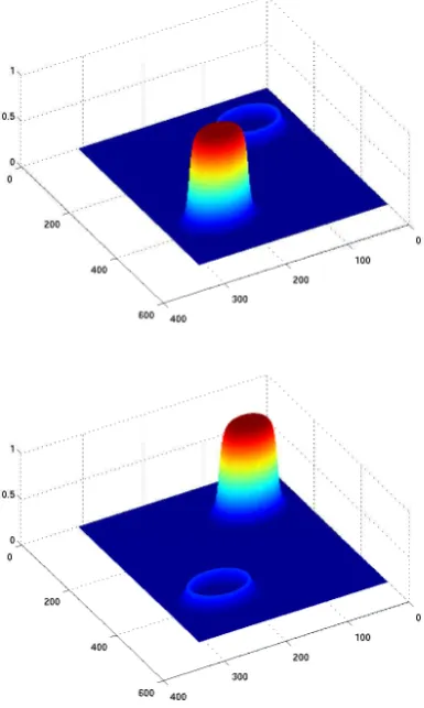
However, the left-hand side is non-vanishing at a (1,2) interface and can give rise to spurious unwanted phases, see Fig. 1. It should be added that with careful choice of potential, see [5], spurious growth can be mitigated (see Appendix C). However, this only holds forN = 3 and the generalisation to
N >3 is not clear within the Lagrange multiplier formulation.
More generally, consider a system ofN phases but only two phases θ1, θ2
present in some region with no interaction with other phases. With θi>2 = 0
the Lagrange multiplier gives
−τθ1˙ = (1− N1)δF
δθ1 − 1
N
δF δθ2
−τθ˙2 = (1− N1)
δF δθ2 − 1 N δF δθ1
−τθ˙i>2 =−N1 ( δF δθ1 + δF δθ2 ) , (12)
Figure 1: The growth from two separated solid seeds of θ2 and θ3, in a melt θ1, using
the Lagrange multiplier model. The left shows θ2 and the right θ3. Surrounding each
3. Development of a new formulation
Having identified at least three defects in the Lagrange multiplier ap-proach (non-reduction to single phase, spurious growth of additional phases and N dependence) this section develops a new formulation that addresses these issues. Specifically an N independent formulation with consistent re-duction to single phase at any (pure) binary phase interface.
The matrix transformation,P, illustrated in (7), can be also looked at as a projection (hence the nomenclature)
P=I−nnT (13)
where, for N = 2,
n= √1
2[1,1]
T
is the outward normal to the line θ2 = 1 −θ1. If we consider the phase
variables, θ1 and θ2 to be Cartesian coordinates, then n has unit length. An alternative to the constant Lagrange multiplier was introduced by [21] in order to eliminate N dependence. It is shown in the appendix that this method is equivalent to a numerical implementation of the constraint used currently, for example, in [22] and [27].
It uses a Lagrange multiplier vector Λi
−τθ˙i =
δF δθi
+ Λi
where
Λi =−θi N
∑
j=1 δF δθj
.
This is equivalent to the projection
P(N) =I(N)−[θ,θ, . . . ,θ]
For example, when N = 2,
P(2) = [
1−θ1 θ1
−θ2 1−θ2 ]
. (14)
3.1. Consistency of form in the phase equations
Here, and in subsequent sections, we make use of the equivalence between differential operators and vector bases (e.g. ∂
∂x ≡ i, ∂
∂y ≡ j etc). Any linear
combination of these bases is termed a contravariant vector. We also use the concept of covariant vectors, which are equivalent to linear combinations of differentials, e.g. dx, dθi etc. Transformations of these objects induced
by maps then follow the chain rule and are equivalent to the perhaps more familiar Jacobian matrices (see for discussion [23]).
Consider the system
−τ∂θi ∂t =
δF δθi
. (15)
In the language of differential geometry, the left-hand side may be written as the push forward (linear map) of the tangent vector on the time line to the phase variable space
∂ ∂t =
∂θi
∂t ∂ ∂θi
.
The left-hand side of (15) is thus a contravariant vector. On the other hand, the right-hand side of equation (15) is a covariant vector
δF = δF
δθj
dθj
(see the book, [23], in the earlier chapters, for a discussion for the necessity of the two types of vectors and Chapter 6 for discussion of Calculus of variations and their connection with covariant vectors).
By equating the two objects in (15) we are saying something about the metric, i.e. drawing an equivalence between the covariant vector basis, dθi,
and contravariant vector basis ∂
∂θi. By making this equivalence we assume
the metric on the phase space is flat and the coordinates, Cartesian. For other coordinates contravariant and covariant vectors are not (automatically) equivalent, e.g. in polar coordinates, the angle, ∂
∂ϕ, is not equivalent to dϕ
4.
To change a covariant vector to a physically equivalent contravariant vector requires a metric g. The system (15) is more correctly written
τ∂θi ∂t =g
ijδF
δθj (16)
4
On the other hand (1/r) ∂
where g is positive definite and symmetric. For Cartesian coordinatesgij =
δij, so the metric is redundant and we can write (15). For an N
−1 di-mensional surface, the metric is represented by a rank N −1 matrix and consequently is singular if, as in the Lagrange multiplier treatment, there are
N coordinates, θi, i∈[1, N] (or non-singular if the unconstrained variables,
φi, i∈[1, N −1] are used).
The constant Lagrange multiplier with metricP(N) is acceptable in this
respect, since it represents the metric of an N −1 dimensional (flat) space embedded in anN dimensional flat space with coordinatesθi, but the vector
Lagrange multiplier, Λi, which gives rise to the matrix (14), is not symmetric
and therefore cannot be formally correct. This is because a projection is a mapping from a contravariant vector to a contravariant vector implying P
has components Pi
j. So the correct way of projecting (16) is
τ∂θi ∂t =P
i jgjk
δF
δθk (17)
and we find that the object
Pik
≡Pi
jgjk = (δij −ninj)gjk =gik−nink
is symmetric. From hereon we assume P with components Pik is an N
×N
symmetric matrix with eigenvalues ≥0. In passing, it is interesting to note the similarity between P in (17) and a projection operator, (denoted πP),
found in [24]
As we have noted, the gij in equation (16) is necessary to balance the
covariant and contravariant vectors. Other tensors, e.g. Tij, can do this,
but a metric transformation retains the physical significance of the object — in this case δF
δθj — and can be constructed from a given specified, smooth,
N−1 dimensional surface in anN dimensional Cartesian space. We give an example of this in Sec. 3.3 where we construct a metric of a line embedded in two dimensional flat space.
3.2. Properties that the mapping must possess
We are now able to lay down a set properties that the matrix (metric)P
must possess
1. Reduces to n < N case when only n phases are present locally in a N
2. The projection must never be zero at any point, as this will inhibit growth from a pure phase.
3. The projection must be symmetric with positive or zero eigenvalues as a result of the consistency requirement between the left-hand and right-hand side components: the vector Lagrange multiplier (14) of [21] fails this test.
4. The metric should be degenerate and continuous: that is, it must map from dimension N to dimension n < N smoothly.
5. Triple points should be active parts of the system: this excludes the model proposed by Steinbach [17].
Possibly the most difficult test to satisfy is the first one. The model [14] fails this, but models such as Steinbach [17] are consistent with this test.
3.3. Mapping for correct reduction to single phase
This section introduces, forN = 2, a mapping fromθ1, θ2to a unit circular arc which induces a metric which reproduces the single phase reduction. This is used in the following section to build a more general mapping for arbitrary
N.
Consider the mapping
r =θ1+θ2,
φ = θ1
r
where r and φ are polar coordinates in a plane. The angle, φ, physically representing the single phase variable and r physically representing the to-tal quantity so that the constraint (5) is represented in this scheme as the restriction in the plane to a unit circular arc. Rearranging we have
θ1 =rφ, θ2 =r(1−φ),
which implies
∂ ∂φ =r
( ∂ ∂θ1 −
∂ ∂θ2
The Euclidean metric in polar coordinates is5
g= ∂
∂r ⊗ ∂ ∂r + 1 r2 ∂ ∂φ⊗ ∂ ∂φ
and so the projected metric on to a circular arc of radius r is
g− ∂
∂r ⊗ ∂ ∂r = 1 r2 ∂ ∂φ ⊗ ∂ ∂φ = ( ∂ ∂θ1 − ∂ ∂θ2 ) ⊗ ( ∂ ∂θ1 − ∂ ∂θ2 )
and since the tensor,P=Pij ∂ ∂θi⊗
∂
∂θj we have that the components are given
by the matrix
P=
[
1 −1
−1 1
]
and in particular when r =θ1 +θ2 = 1 the parameter φ is arc length. This
agrees with the single phase formulation (6).
There are other mappings, however, that do this. Consider the mapping in Cartesian coordinates x, y
x= √1
2θ1, y= 1
√
2θ2
then by a similar process the metric on the surface, θ1 +θ2 = 1 (or x+y= 1/√2), is also
P=
[
1 −1
−1 1
]
since a unit Cartesian basis on the surface is
1 √ 2 ( ∂ ∂x − ∂ ∂y ) = ∂ ∂θ1 − ∂ ∂θ2.
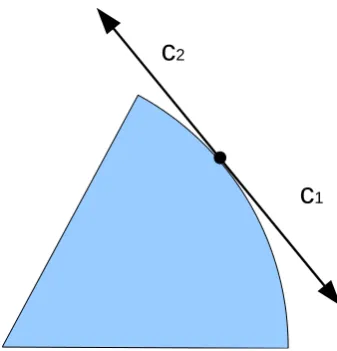
Figure 2: On the unit length circular arc we show two unit length (not to scale) vectors defined at one point. A metric of the arc may be formed from a tensor combination of either or both vectors.
pure interface. To this end we first write the above in a form that may be generalised.
Let us define two unit vectors on the arc (see Fig. 2)
c1 ≡ ∂ ∂θ1 −
∂ ∂θ2
, c2 ≡ ∂ ∂θ2 −
∂ ∂θ1
.
Then we find that we can trivially write the metric on the arc as
P=αc1⊗c1+ (1−α)c2⊗c2
for any α. In particular we may write
P=θ1c1 ⊗c1 +θ2c2 ⊗c2
=
2 ∑
i=1
θici⊗ci (18)
We can also trivially write
P= θ1θ2
(1−θ1)(1−θ2)
[
1 −1
−1 1
]
(19)
5
In Cartesian coodinates x, y the metric of a flat plane is g= ∂ ∂x⊗
∂ ∂x +
∂ ∂y ⊗
Generalisations to N >2 of these two equivalent formulations, (18) and (19) for N = 2 are exploited in the following subsections.
3.4. Proposed multi-phase formulation A
We now develop a natural generalisation of the N = 2 case, (18), to
N > 2. For N = 2 we could interpret the construction as a mapping from the (straight) line segment θ1 +θ2 = 1 to a circular arc to induce a met-ric. Extending this approach to N = 3 we consider a mapping from the 2 dimensional simplex θ1 +θ2 +θ3 = 1 to a 2 dimensional non flat surface – in particular a sphere. In this way, under the constraint,θi form barycentric
coordinates on the simplex and map to spherical barycentric coordinates on a sphere 6. We then modify the result so that the metric reduces to that of N = 2 for a pure binary interface.
We first aim to establish a geodesic coordinate system on a spherical triangular simplex. Consider first longitude and latitude on a sphere- θ, ϕ
respectively. Then θ parametrises a set of geodesics labelled by ϕ, and con-versely the curves parametrised by ϕ intersect these curves at constant val-ues of θ. Limiting the domain to an eighth sphere (positive x, y, z) with
θ, ϕ∈[0, π/2], we have an equilateral spherical triangle with three poles x= (1,0,0),(0,1,0),(0,0,1) in Cartesian coordinates, where each geodesic of con-stantϕconventionally begins at the pole (0,0,1) and ends at (cosϕ,sinϕ,0). We can equally well choose the other two poles as the origin of the geodesics. Let us label these three coordinates systems (θ1, ϕ1),(θ2, ϕ2),(θ3, ϕ3). Note that the duplicate use here of the symbol θi for angle as well as for the phase
field is no coincidence. The three sets of geodesicsC1(θ1, ϕ1),C2(θ2, ϕ2),C3(θ3, ϕ3)
are generated by and are integral curves of three vector fields, c1,c2 and c3
respectively. Considering the spherical equilateral triangle as a mapping from a flat equilateral triangle, then the straight lines emanating from the vertices of the flat triangle map to geodesics on the spherical triangle. The barycen-tric coordinates of a point on the flat triangle, say (λ1, λ2, λ3), correspond exactly to geodesic distances (π/2−θ1, π/2−θ2, π/2−θ3) to each respective vertex. If we reverse the direction of the parameter θi so that the integral
curves begin at the equator and move towards the poles then the relation is
θi = (π/2)λi.
6
However, we still interpret the vector fields ∂
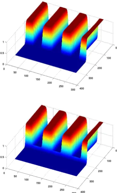
Figure 3: Eutectic growth of solid θ2 for the proposed model (left) and the Lagrange
multiplier (right). We see on the right that there is spurious growth of solid θ2 at the
interface between solid θ3 and the liquid θ1. This is not present at all in the proposed
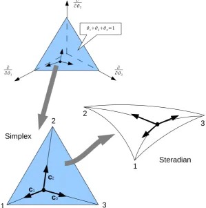
Figure 4: Mapping from the N = 3 dimensional space to the flat simplex (implementing the constraint) to the steradian (implementing the metric). The unit vectorscipoint along the line to the respective vertices,i. The distance between a vertex,xi and a point,x, is given by the distance on the steradian, 1−θi. As a point approaches an edge, sayθ2→0,
Moving on to the spherical triangle with unit geodesic edges (a stera-dian) and with the reversed direction of parametrisation the correspondence becomes λi =θi. This implies that the distance from a vertex ito a general
point is given by 1 −θi. Interestingly, the distances to a point in the flat
triangle from the vertices do not have such a neat relation to the barycentric coordinates as the spherical barycentric coordinates do. See [25] for issues on creating spherical barycentric coordinates, in particular the ‘coordinate’ system we have created does not have all the properties that a true barycen-tric coordinate system has, e.g. lines of constant θ1 are not geodesics and therefore not parametrised by θ2 or θ3.
The three unit geodesic vector fields on the unit spherical triangle corre-spond to
ci = xi−x 1−θi
on the flat triangle, where the barycentric position,
x=∑θixi,
with each pure phase given by
x1 = [1,0,0]T,x2 = [0,1,0]T,x3 = [0,0,1]T.
In component form ci is thus
(ci)j ≡cij =
δij −θj
1−θi
, (20)
We know this because the geodesics from any point to any vertex on the spherical triangle map to straight lines from x to each vertex xi on the flat triangle. So a tangent to each geodesic maps to a tangent to each straight line – see Fig. 4. To make this tangent vector unit length we divide by the geodesic distance of the point on the spherical triangle, corresponding to x
on the flat triangle, from the vertices, i.e. 1−θi. The relation between the
vectors on the N−1 simplex ci and theN dimensional space is
ci =cij
∂ ∂θj
.
will give a metric for a curve. With this in mind we construct a metric from the three vector fields, for an arbitrary point on the simplex, as follows:
P=
N
∑
j
θjcj⊗cj (21)
where the coefficients, θi of P, amount to a postulate, without which we
would have no degeneracy to local regions n < N, where n is the number of phases present in a local region. In component form the metric is
Pij =
N
∑
k
θkckickj (22)
Note that, for N = 3, by construction when say θ2 = 0, so that θ1+θ3 = 1
and c3 =−c1 , then the metric degenerates to
P|θ2=0 =θ1c1⊗c1+θ3c3⊗c3
= (θ1+θ3)c1⊗c1
=c1⊗c1
=
( ∂ ∂θ1 −
∂ ∂θ3
) ⊗
( ∂ ∂θ1 −
∂ ∂θ3
)
. (23)
single phase formulation. To illustrate this we give P for this case explicitly
P(4) = θ1
(1−θ1)2
(1−θ1)2 −(1−θ1)θ2 −(1−θ1)θ3 −(1−θ1)θ4
−(1−θ1)θ2 θ22 θ2θ3 θ2θ4
−(1−θ1)θ3 θ2θ3 θ32 θ3θ4
−(1−θ1)θ4 θ2θ4 θ3θ4 θ42
+ θ2
(1−θ2)2
θ12 −(1−θ2)θ1 θ3θ1 θ4θ1
−(1−θ2)θ1 (1−θ2)2 −(1−θ2)θ3 −(1−θ2)θ4
θ3θ1 −(1−θ2)θ3 θ32 θ3θ4
θ4θ1 −(1−θ2)θ4 θ3θ4 θ42
+ θ3
(1−θ3)2
θ12 θ1θ2 −(1−θ3)θ1 θ4θ1
θ1θ2 θ22 −(1−θ3)θ2 θ2θ4
−(1−θ3)θ1 −(1−θ3)θ2 (1−θ3)2 −(1−θ3)θ4
θ4θ1 θ2θ4 −(1−θ3)θ4 θ42
+ θ4
(1−θ4)2
θ12 θ1θ2 θ3θ1 −(1−θ4)θ1
θ1θ2 θ22 θ2θ3 −(1−θ4)θ2
θ3θ1 θ2θ3 θ32 −(1−θ4)θ3
−(1−θ4)θ1 −(1−θ4)θ2 −(1−θ4)θ3 (1−θ4)2
(24)
which indeed reduces to
1 −1 0 0
−1 1 0 0
0 0 0 0
0 0 0 0
1/3 we obtain
1/2 −1/4 −1/4 0
−1/4 1/2 −1/4 0
−1/4 −1/4 1/2 0
0 0 0 0
.
This matrix has a singularity when any phase equals unity. There are a number of ways of resolving this which are discussed in Section 3.6 after we introduce an alternative formulation (model B).
3.5. Proposed multi-phase formulation B
It is not suggested that the proposed mapping and resulting projection, Sec. 3.4, is the only acceptable approach to constraining the phase variables. Further examples that do not reduce to single phase are given in Appendix D. We give another example here which generalises the N = 2 case via equation (19). For N = 3, we can construct Pas follows:
P= θ1θ2
(1−θ1)(1−θ2)
1 −1 0
−1 1 0
0 0 0
+
θ2θ3
(1−θ2)(1−θ3)
0 0 0
0 1 −1
0 −1 1
+
θ3θ1
(1−θ3)(1−θ1)
1 0 −1
0 0 0
−1 0 1
.
where we note that if, say, θ3 = 0 we obtain the N = 2 case. The general case follows as
P=
N
∑
j=2
j−1 ∑
i=1
θiθj
(1−θi)(1−θj)
(xi−xj)⊗(xi−xj),
where xi are the barycentric coordinates of each vertex, i.e. (xi)j = δij, so
that in components, (a, b)
Pab = N
∑
j=2
j−1 ∑
i=1
θiθj
(1−θi)(1−θj)
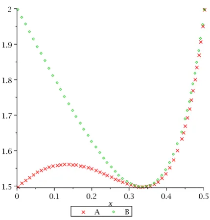
Figure 5: Red crosses show the value of tr(P) for a path joining vertexθ3= 1 to the middle
of the interface opposite. The trace at the vertex differs from the value of 2 for model A on this path even though it equals two on the adjoining edges (θ1 = 0 and θ2 = 0).
This formulation (B) has the advantage of being lower order in θi than
that of formulation A of Sec. 3.4. The behaviour on an interface and at a triple point is identical, but otherwise they differ.
3.6. Ill-defined P for a pure phase
Models A and B, as they stand, both suffer from being ill-defined at any vertex, θi = 1. This is due to a feature of our construction that, at the
vertices, P depends on the path. For example, with N = 3, and θ1 = 1 we find P degenerates to two matrices for paths along the two adjoining edges
θ3 = 0 andθ2 = 0:
P|θ3=0 =
1 −1 0
−1 1 0
0 0 0
P|θ2=0 =
1 0 −1
0 0 0
−1 0 1
. (26)
Thus we require, in addition to the definition (21), to define unique matrices at each vertex. Alternatives such as enforcingθi <1 via the initial condition,
the use of a small parameter in local averaging, or modifying the potential are all problematic.
Many candidates for the value ofPat the vertices fail, including: P=0, which inhibits growth; andP=I−U/N, which introduces spurious growth. However, we found
Pvertex = 2I−U, if 1−θi < δ, for any i, (27)
where the small parameter, δ ≪ 1, did not significantly alter results7. To
discuss this we write this out for N = 3
Pvertex ≡
1 −1 −1
−1 1 −1
−1 −1 1
and assume that θ3 and its gradients vanish. Thus,
δF δθ3 = 0
7
For a range of 10−10to 10−14inδwe found the steady state growth rate was effectively
Consequently the third column plays no role and ˙θ1 and ˙θ2 reduce correctly to a binary phase formulation. On the other hand
τθ3˙ = δF
δθ1 + δF δθ2
has a right hand side which is non-zero in general. In fact, from (11) we see that the contribution from the potential is zero leaving, for θ1 = 1:
τθ3˙ = 2(∇θ1· ∇θ1) +∇2θ1.
Now, since θ1 = 1 we must have ∇θ1 = 0 and∇2θ1 ≤0 implying
τθ3˙ ≤0.
Assuming negative contributions are trapped numerically (if θi < 0 then
θi = 0) this contribution is effectively ignored.
Hence, we have shown that when θ3 and all its gradients are vanishing, then at one of the other vertices, we find that
Pvertex ≡
1 −1 −1
−1 1 −1
−1 −1 1
is indistinguishable from
1 −1 0
−1 1 0
0 0 0
The general case, (27), easily follows.
3.7. Some properties of models A and B
This section considers the models from the perspective of eigenvectors and eigenvalues of the matrixPin order to see the effect on the system. The interface defined by θ3 = 0 gives the matrix
P=
1 −1 0
−1 1 0
0 0 0
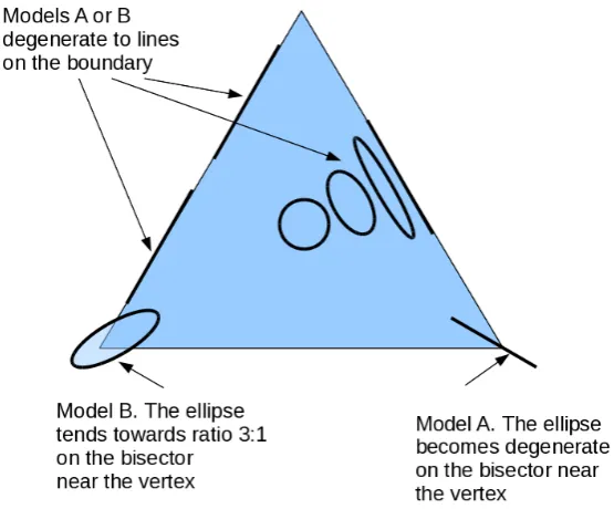
normal to the interface. In general P has the double effect of projecting out the normal component and rescaling the components of the vector along the two eigenvectors. Representing P at any point on the simplex by an ellipse with major and minor axes of lengths and direction given by the eigenvalues and eigenvectors, we can view the action of P in the centre as a circle and at an interface a degenerate ellipse — a line (see Fig. 6).
Consider a typical path on an N = 3 simplex given by
x(t) = [θ1 =t, θ2, θ3 = 1−2t], t∈[0,1
2]. (28)
We are interested in the property of P as we approach the vertex θ3 = 1 as
t tends to zero. We find, for formulation A that, in the limit, the effect of
P once again degenerates to a line (this time of length 3/2) pointing along the path defined by (28). However, in formulation B we find that P is an ellipse with major axis of length 3/2 pointing along the line and minor axis of length 1/2. We find this type behaviour along all paths approaching the vertices.
By inspecting the trace, tr(P) = ∑N
i Pii ,for both models we find for
formulation A that tr(P) is path dependent at a vertex. This is illustrated in Fig. 5, which shows tr(P) for both models for a path θ1 =x, θ2 =x, θ3 = 1−2x, i.e. from vertex θ3 = 1 to a point on the interface opposite (where tr(P) = 2) via the triple point (where tr(P) = 3/2).
A constant value of 2 for the trace of P throughout the simplex may be enforced for both models by the transformation
P→Pˆ = 2 P tr(P).
This modification of either model was found to make no significant change to eutectic or single phase growth.
4. A numerical comparison of models 4.1. Growth velocity comparison for a single seed
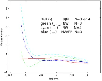
Figure 8: P´eclet number, 1
2× Velocity × Radius/Diffusivity of liquid (1×10− 9
)m2 /s
against log10(t), for: The proposed model ( A or B withN = 3 orN = 4 are all identical
in this test), Lagrange multiplier model used in Nestler-Wheeler (NW)N = 3 and (NW)
N = 4. We also include the Lagrange multiplier model with Folch-Plapp type change to the potential (NW/FP) N = 3 which avoids spurious phase growth. The first 2000 time steps (with ∆t = 3.5×10⁻⁹) are suppressed because of extreme transient behaviour in
In the new models A or B (BJM) there is no difference in growth velocity, whatever the value of N. On the other hand the Lagrange multiplier model (NW) behaves differently, as expected, depending on N. We also include a modified potential into the NW model to make the potential have a maximum in the middle of the simplex in the manner of [5] (FP).
To calculate the interface velocity we use the formulation
vn=
xn−xn−1
∆t
where the x position of the interface at time tn is given by
xn=
∫∞
O xh(θ1(x, tn)) dx
∫∞
O h(θ1(x, tn)) dx
whereOis the origin of the seed,θ1(x, tn) is the amount of liquid at the point
x at time tn, and the function (interface selector)
h(θ)≡16θ2(1−θ)2
is used to isolate the interface.
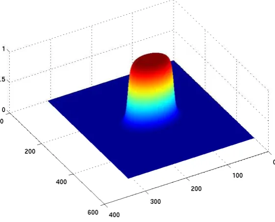
A snap shot of θ2 in the simulation is illustrated in Fig. 7. Fig. 8 illustrates the differing growth rates using the P´eclet number, 1
2×Velocity×
Radius/Diffusivity, for the models and also, detrimentally for the NW model, we find differing growth rates for N = 3 and 4 cases. In BJM there is no difference between N = 3 and N = 4 the growth rates being identical. The simulation reveals that BJM is also more stable than the Lagrange multiplier model(s). We also ran a simulation for the Lagrange multiplier formulation with a modified potential (NW/FP) to eliminate spurious phases, but even in this case there is significant difference in growth rate between this model and the proposed model (BJM). We did not run a simulation for N = 4 with the modified potential NW/FP because as commented in [12]: . . . a special type of a potential function that guarantees the stability of dual interfaces is constructed(in [5]).This formulation, however, is restricted to triple junctions and will be difficult to generalize.
4.2. Eutectic growth differences between models A and B
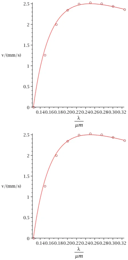
Figure 9: Velocity as a function of eutectic width (circles A(left) B(right)) against the solid line, 1
λ(1− λ∗
the eutectic solidifies more rapidly with increased width until a maximum,
λ = 2λ∗, is reached. This “velocity scaling law” can be shown to be:
v ∝ 1 λ
(
1−λ
∗
λ )
.
Fig. 9 shows the analytical relation (solid line) against the data for different
λ, for an undercooling of 6.9K. Both models A and B fit well through the range from 1 to 3 times the minimum spacingλ→λ∗. Modifying the models
to ensure trace 2 does not have any significant effect and there is no significant observed difference between models A and B in this test. It has been shown in [21] that the constant Lagrange multiplier model and vector Lagrange multiplier do not reproduce this scaling correctly, whereas the model of [19] does successful reproduce the law.
5. Conclusion
We have proposed two multi-phase formulations that reduce to standard single phase, have no N dependence, do not generate spurious additional phases at binary interfaces and fit the velocity scaling law well. Moreover, they use a simple potential for general N, given in [14].
Towards these formulations we first explored properties of the Lagrange multiplier method for multi-phase fields and identified the unphysical aspects: non reduction to single phase, the generation of additional spurious phases andN dependence. In particular we have shown that the Lagrange multiplier method is equivalent to a projection with a specified normal which assumes a Cartesian metric on the phase variables. By relaxing this assumption we exploit the extra freedom to construct a projection that allows growth of a pure seed into the melt without influence of the remaining phases.
Reduction to single phase is achieved by the introduction of a symmet-ric matrix, which degenerates to a single non-zero eigenvalue when only two phases are present. Thus the form of the potential is not critical at a pure interface. However, reduction to single phase and N independence are con-ditions that necessarily create an ambiguity when the phase is pure. For example, a point of pure melt θ1 = 1 cannot simultaneously be a single phase formultion for more than one solid growth. This reveals itself in the proposed formulation as being ill-defined at these points. We resolved this by specifying a particular matrix,Pvertex, at these points consistent with the
Because the new formulation reduces exactly to the single phase formu-lation at a pure binary interface more elaborate treatment of the latter, e.g. solute anti trapping, may be imported into multi-phase field modelling. This is a subject for future research.
5.1. Summary of the proposed multi-phase field models A and B
For the convenience of the reader we finish with a summary of the pro-posed model.
• We use free energy in equation (1) with the potential, equation (2)
• The evolution of concentration is given by (4)
• The constraint (5) is applied to unconstrained phase field equations, (3), by
−τθ˙ =PδF
δθ
• where P is an N ×N symmetric matrix given in component form by two proposed formulations:
– Model A: (22) withcij given by (20); – Model B: (25)
• Because these formulations are ill-defined at pure phases (verticesθi =
1) we specify a matrix (27) if any of the phases approaches unity.
Both models A and B perform equally well in simulations and far better than with the Lagrange multiplier approach for general N 8.
Appendix A. Proof of the equivalence of (10) and the Lagrange multiplier approach
This section shows the equivalence between the Lagrange multiplier method of constraining the N equations and that of using any mapping θ = θ(φ)
8
that automatically preserves the constraint ∑
iθi = 1. Since the Lagrange
multiplier pe se is traditionally used in pure minimisation problems (i.e. no time dependence) it is not necessarily obvious that the two approaches are identical, although the identification of the Lagrange multiplier as a projec-tion (equaprojec-tion (13)) strongly suggests that they are.
We need to show that9
JTJφ˙ = δF
δφ, (A.1)
where the entries
N
∑
i=1
Jij = 0, j ∈[1, N −1],
is equivalent to
˙
θ=PδF
δθ
with P given by
P≡I− 1
NU,
and U defined as anN ×N matrix with unit entries. First we note that
˙
θi =
∂θi
∂φj
˙
φj ⇒θ˙ =Jφ˙ (A.2)
and similarly
δF δφ =J
TδF
δθ. (A.3)
So that constraining the system of N equations
˙
θ= δF
δθ
9
to an N −1 system by writing θ = θ(φ) and using (A.2) and (A.3) results in the N −1 independent equations (A.1)
JTJφ˙ = δF
δφ.
Using (A.2) and (A.3), we can rearrange this as the N dependent equations
˙
θ=QδF
δθ.
where we define
Q≡J(JTJ)−1JT (A.4)
Hence, we need to show that P ≡ I− U/N = J(JTJ)−1JT
≡ Q. To prove this result it is sufficient to prove the equality for the symmetric (N−
1)×(N −1) matrix, ˆP, formed from the independent rows and columns of
P. We choose, without loss of generality, that row and columnN are deleted to form ˆPand similarly the Nth row of J to form ˆJ etc—note that unlike J
and P, the rank N −1 matrices ˆJ and ˆP are invertible. Using
(JTJ)ij = N
∑
k=1 JkiJkj
=
N−1 ∑
k=1
JkiJkj +JN iJN j
=
N−1 ∑
k=1
JkiJkj +
(N−1 ∑
m=1 Jmi
) (N−1 ∑
n=1 Jnj
)
=(JˆTJˆ+ ˆJTUˆJˆ) ij
we find from (A.4)
ˆ
Q≡Jˆ( ˆJTJˆ+ ˆJTUˆJˆ)−1JˆT.
Using the notation ˆJ−T
≡(ˆJT)−1 we find
so that
ˆI= ( ˆJTJˆ+ ˆJTUˆJˆ)J−1QˆˆJ−T
= ˆJTQˆJˆ−T + ˆJTUˆQˆJˆ−T
= ˆQ+ ˆUQˆ
= (ˆI+ ˆU) ˆQ
implying
ˆ
Q= (ˆI+ ˆU)−1 Now
(ˆI− 1
NUˆ)(ˆI+ ˆU) = ˆI+ ˆU−
1
NUˆ −
1
NUˆUˆ
= ˆI+ ˆU− 1
NUˆ −
N −1
N Uˆ
= ˆI
implying
ˆI− 1
NUˆ = (ˆI+ ˆU)
−1
and so
ˆ
Q = ˆI− 1
NUˆ = ˆP
giving P=Q as required.
Appendix B. Variational derivative calculations
The purpose of this appendix is to show how the variational derivative of the gradient contribution enter the giverning equations (11).
We wish to find δG
δθk where
G=
∫
Ω
with
h= 12
N
∑
j=2
j−1 ∑
i=1
Γij|θi∇θj−θj∇θi|2
Then
δG δθk
= ∂h
∂θk − ∇ ·
∂h ∂∇θk
Writing
rij ≡θi∇θj−θj∇θi
we find ∂h ∂θk = N ∑ j=2
j−1 ∑
i=1
Γijrij
· ∂rij ∂θk
=
N
∑
j=2
j−1 ∑
i=1
Γijrij ·(δik∇θj−δjk∇θi)
=
N
∑
j=2
Γkjr
kj ·(∇θj−δjk∇θk)
=
N
∑
j̸=k
Γkjrkj
· ∇θj.
A similar calculation gives
∂h ∂∇θk
=
N
∑
j=2
j−1 ∑
i=1
Γijrij ∂rij
∂∇θk
=−
N
∑
j̸=k
Γkjrkjθ j.
and thus
−∇ · ∂∂h ∇θk
=
N
∑
j̸=k
Hence
δG δθk
=
N
∑
j̸=k
Γkj(2rkj · ∇θj+θj∇ ·rkj)
=
N
∑
j̸=k
Γkj{2(θk∇θj −θj∇θk)· ∇θj + (θk∇2θj −θj∇2θk)θj}
Appendix C. A modified potential to suppress spurious growth in the Lagrange multiplier model
This section examines a modification to the potential that mitigates spu-rious phases in the Lagrange multiplier approach.
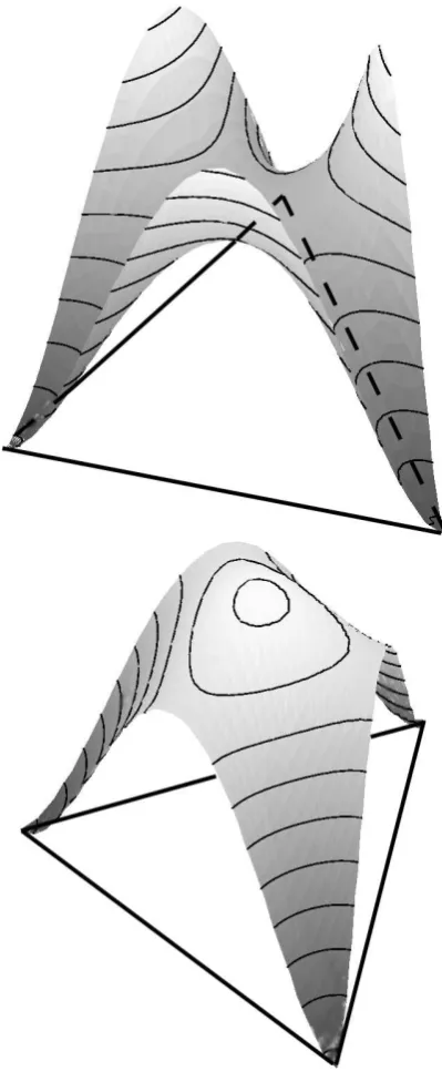
See Fig. C.10 showing the Nestler Wheeler potential on the left and the Folch-Plapp potential on the right. The drawback for the NW potential is that there is a gradient away from an interface (an edge of the simplex) towards the centre. The Folch Plapp potential avoids this, whilst taking care not to create a gradient out of the simplex.
The barrier contribution to the potential for N = 3 is
fbarrier =
3 ∑
k=2
k−1 ∑
j=1
Wjkθj2θ2k
if we modify this potential
fbarrier =
3 ∑
k=2
k−1 ∑
j=1
Wjk(θ2jθ2k+αθ1θ2θ3) (C.1)
where α is a new parameter. We find for θ3 = 0
∂fbarrier ∂θ1
= 2W12θ1θ22
∂fbarrier
∂θ2 = 2W12θ2θ 2 1
∂fbarrier ∂θ3
so that, for α = 1, with the Lagrange multiplier this contribution to the growth of phase 3 is
2 3
∂fbarrier
∂θ3 −
1 3
(
∂fbarrier
∂θ1 +
∂fbarrier ∂θ2
)
= 0
since θ1 +θ2 = 1. So the addition of the ‘hump’ into the potential negates its contribution to the growth of θ3, but there still remains contributions
to spurious growth due to the non-potential term. However, this can be mitigated by choosing α >1 and sufficiently large, relying on an infinite well at the simplex boundary.
Appendix D. Alternative formulations for P
We state without comment or justification two possible forms forPwhich, though they do not reduce correctly to the standard single phase formulation, do demonstrate alternative approaches to implementing the constraint that avoid N dependence and spurious phase generation:
1.
Pij =θiδij −θiθj;
2.
Pij =d2∇θi· ∇θj,
with d a parameter of dimension length commensurate with phase width.
Appendix E. Numerical implementation of the constraint
Following a suggestion by the reviewers of this article we were asked to comment on the method of [22] who in turn use the method of [27] for implementing the constraint. Consider the equations with constants assumed unity for simplicity:
˙
θi =
δF δθj
Using explicit Euler for time stepping for illustration, Hirouchi et al imple-ment the constraint as follows:
At time step t = tn+1 the equation is computed first without the
con-straint
θni+1 ←θ n i + ∆t
δF δθn
i
The constraint is then imposed by
θn+1
i ←
θn+1
i ∑ jθ n+1 j .
To analyse this let us rewrite this process into one line
θn+1
i =
θn
i + ∆tδθδFn i
∑
jθ n j + ∆t
∑ j δF δθn j = θ n
i + ∆tδθδFn i
1 + ∆t∑
j δF δθn
j
which for small ∆t can be written
θn+1
i −θni
∆t ≈
δF δθn
i
−θn i ∑ j δF δθn j .
We now see that this is the numerical approximation to
˙
θi =
δF δθi −
θi
∑
j
δF δθj
which is the vector Lagrange multiplier approach mentioned in [21].
References
[1] A. M. Mullis, A study of kinetically limited dendritic growth at high undercooling using phase-field techniques, Acta Materialia 51 (2003) 1959–1969.
[3] R. Kobayashi, Modeling and numerical simulations of dendritic crystal growth, Physica D: Nonlinear Phenomena 63 (1993) 410–423.
[4] A. A. Wheeler, W. J. Boettinger, G. B. McFadden, Phase-field model for isothermal phase transitions in binary alloys, Physical Review A 45 (1992) 7424–7439.
[5] R. Folch, M. Plapp, Quantitative phase-field modeling of two-phase growth, Physical Review E 72 (2005) 011602+.
[6] Y. Sun, C. Beckermann, Effect of solidliquid density change on dendrite tip velocity and shape selection, Journal of Crystal Growth 311 (2009) 4447–4453.
[7] L. Brush, A phase field model with electric current, Journal of Crystal Growth 247 (2003) 587–596.
[8] A. M. Mullis, R. F. Cochrane, A phase field model for spontaneous grain refinement in deeply undercooled metallic melts, Acta Materialia 49 (2001) 2205–2214.
[9] T. B¨orzs¨onyi, T. T. Katona, Buka, L. Gr´an´asy, Dendrites Regularized by Spatially Homogeneous Time-Periodic Forcing, Physical Review Letters 83 (1999) 2853–2856.
[10] A. Wheeler, B. Murray, R. Schaefer, Computation of dendrites using a phase field model, Physica D: Nonlinear Phenomena 66 (1993) 243–262.
[11] J. Warren, W. Boettinger, Prediction of dendritic growth and microseg-regation patterns in a binary alloy using the phase-field method, Acta Metallurgica et Materialia 43 (1995) 689–703.
[12] I. Steinbach, Phase-field models in materials science, Modelling and Simulation in Materials Science and Engineering 17 (2009) 073001+.
[13] B. Nestler, A. A. Wheeler, L. Ratke, C. St¨ocker, Phase-field model for solidification of a monotectic alloy with convection, Phys. D 141 (2000) 133–154.
[15] H. Garcke, B. Nestler, B. Stoth, On anisotropic order parameter models for multi-phase systems and their sharp interface limits, Physica D: Nonlinear Phenomena 115 (1998) 87–108.
[16] L. Vanherpe, F. Wendler, B. Nestler, S. Vandewalle, A multigrid solver for phase field simulation of microstructure evolution, Mathematics and Computers in Simulation 80 (2010) 1438–1448.
[17] I. Steinbach, F. Pezzolla, B. Nestler, M. Seeszelberg, R. Prieler, G. J. Schmitz, J. L. L. Rezende, A phase field concept for multiphase systems, Physica D (1996) 135–147.
[18] J. Tiaden, The multiphase-field model with an integrated concept for modelling solute diffusion, Physica D: Nonlinear Phenomena 115 (1998) 73–86.
[19] I. Steinbach, A generalized field method for multiphase transformations using interface fields, Physica D: Nonlinear Phenomena 134 (1999) 385– 393.
[20] A. Choudhury, M. Plapp, B. Nestler, Theoretical and numerical study of lamellar eutectic three-phase growth in ternary alloys, Physical Review E 83 (2011) 051608+.
[21] R. Green, James, Thesis — A Comparison of Multiphase Models and Techniques, Leeds University, School of Computing and Institute for Materials Research, 2007.
[22] T. Hirouchi, T. Tsuru, Y. Shibutani, Grain growth prediction with inclination dependence of 110 tilt grain boundary using multi-phase-field model with penalty for multiple junctions, Computational Materials Science 53 (2012) 474–482.
[23] D. Lovelock, H. Rund, Tensors, Differential Forms, and Variational Prin-ciples, Dover Publications, 1989.
[25] T. Langer, A. Belyaev, H.-P. Seidel, Spherical Barycentric Coordinates, 2006.
[26] D. A. Porter, D. A. Porter, K. Easterling, Phase Transformations in Metals and Alloys, Chapman & Hall, 1992.