PSA based multi objective evolutionary algorithms

This is a repository copy of

PSA based multi objective evolutionary algorithms

.

White Rose Research Online URL for this paper:

http://eprints.whiterose.ac.uk/98424/

Version: Accepted Version

Proceedings Paper:

Salomon, S., Domínguez-Medina, C., Avigad, G. et al. (4 more authors) (2014) PSA based

multi objective evolutionary algorithms. In: EVOLVE - A Bridge between Probability, Set

Oriented Numerics, and Evolutionary Computation III. EVOLVE, August 2012, Mexico City,

Mexico. Studies in Computational Intelligence, 500 . Springer , pp. 233-259.

https://doi.org/10.1007/978-3-319-01460-9_11

[email protected] https://eprints.whiterose.ac.uk/

Reuse

Unless indicated otherwise, fulltext items are protected by copyright with all rights reserved. The copyright exception in section 29 of the Copyright, Designs and Patents Act 1988 allows the making of a single copy solely for the purpose of non-commercial research or private study within the limits of fair dealing. The publisher or other rights-holder may allow further reproduction and re-use of this version - refer to the White Rose Research Online record for this item. Where records identify the publisher as the copyright holder, users can verify any specific terms of use on the publisher’s website.

Takedown

If you consider content in White Rose Research Online to be in breach of UK law, please notify us by

Shaul Salomon1_{, Christian Dom´ınguez-Medina}2_{, Gideon Avigad}3_{, Alan}

Freitas4_{, Alex Goldvard}3_{, G¨unter Rudolph}5_{, Oliver Sch¨utze}6_{, and Heike}

Trautmann7

Abstract It has generally been acknowledged that both proximity to the

Pareto front and a certain diversity along the front, should be targeted when using evolutionary multiobjective optimization. Recently, a new partitioning mechanism, the Part and Select Algorithm (PSA), has been introduced. It was shown that this partitioning allows for the selection of a well-diversified set out of an arbitrary given set, while maintaining low computational cost. When embedded into an evolutionary search (NSGA-II), the PSA has sig-nificantly enhanced the exploitation of diversity. In this paper, the ability of the PSA to enhance evolutionary multiobjective algorithms (EMOAs) is further investigated. Two research directions are explored here. The first one deals with the integration of the PSA within an EMOA with a novel strategy. Contrary to most EMOAs, that give a higher priority to proximity over diver-sity, this new strategy promotes the balance between the two. The suggested algorithm allows some dominated solutions to survive, if they contribute to diversity. It is shown that such an approach substantially reduces the risk of the algorithm to fail in finding the Pareto front. The second research di-rection explores the use of the PSA as an archiving selection mechanism, to

1 _{Department of Automatic Control and Systems Engineering, University of Sheffield,}

Mappin Street, Sheffield S1 3JD, UK. e-mail: [email protected]

2 _{Computer Research Center, CIC-IPN, Av. Juan de Dios B´atiz Esq. Miguel Othon de}

Mendizabal, 07738, Mexico City, Mexico. e-mail: [email protected]

3 _{ORT Braude College of Engineering, Snunit 51, Karmiel 21982, Israel. e-mail:}

[email protected], [email protected]

4 _{Programa de P´os-Gradua¸c˜ao em Engenharia El´etrica - Universidade Federal de Minas}

Gerais - Av. Antˆonio Carlos 6627, 31270-901, Belo Horizonte, MG, Brasil. e-mail: [email protected]

5 _{TU Dortmund University, 44227 Dortmund, Germany. e-mail:}

[email protected]

6_{Computer Science Department, CINVESTAV-IPN, Av. IPN 2508, Col. San Pedro}

Zaca-tenco, Mexico City, Mexico. e-mail: [email protected]

7 _{Information Systems and Statistics, University of M¨unster, Leonardo-Campus 3, 48149}

M¨unster, Germany. e-mail: [email protected]

improve the averaged Hausdorff distance obtained by existing EMOAs. It is shown that the integration of the PSA into NSGA-II-I and∆p-EMOA as an

archiving mechanism leads to algorithms that are superior to base EMOAS on problems with disconnected Pareto fronts.

1 Introduction

In many real-world applications, several objectives must be optimized at the same time, leading to a multi-objective optimization problem (MOP). Math-ematically, a MOP can be stated as follows:

min

x∈QF(x) (1)

whereQ⊂Rdis a domain ind-dimensional real space,F(x) is defined as the vector of thekobjective functions:

F(x) = [f1(x), . . . , fk(x)]T

where each objective functionfi(x), i= 1, . . . k, maps the vectorx∈RdtoR.

The set of optimal solutions of the problem (1) is usually called the Pareto set

predominant approach used to exploit proximity to the true Pareto front. Diversity is exploited by different approaches that can be classified into three main categories. The first treats diversity as a property of a set and evolves sets with a good diversity. The diversity can be measured according to the accumulated distances between the members of the set [8], [9], or indirectly by the hypervolume measure [10] or the averaged Hausdorff distance∆p[11].

Algorithms in the second category treat diversity as a property of each indi-vidual according to the density of solutions surrounding it. Fitness sharing of NPGA [12], crowding distance of NSGA-II [13], the diversity metric based on entropy [14] and the density estimation technique used in SPEA2 [15] are examples of this category. Algorithms of the third category decompose the multi-objective problem into a number of single objective problems (scalar-ization). Each of these problems ideally aims for a different zone on the Pareto front such that the set of solutions to the auxiliary problems form a diverse set of optimal solutions. MOEA/D [16] is probably the most famous method within this category. A recent method from this category [17] combines Pareto dominance with Chebyshev decomposition for the selection process.

When selection takes place for the sake of exploiting proximity and di-versity, proper selection criteria must be formulated, in order to achieve a balance among these two inspirations. Such a balance is not easy to achieve because it has been shown that these motivations are contradicting [18]. An improvement in one usually involves regression in the other. A balance be-tween proximity and diversity within the exploitation phase has been targeted in various ways. One way is to select the elite population by pure truncation selection. In truncation selection, the algorithm sorts all individuals based on their domination level and includes the first individuals as the elite popula-tion. Truncation selection is exploited in many EMOAs, such as NSGA-II [13] and SPEA2 [15]. In those algorithms the exploitation of proximity takes over that of diversity as the solutions are primarily chosen based on domination relations. Some efforts to overcome this drawback have been made e.g., using the Balanced Truncation Selection (BTS) [7] within MIDEA (Multi-objective Mixture based Iterated Density Estimation Evolutionary Algorithm). In that algorithm, the exploitation of diversity can be improved by a tuned trunca-tion threshold. The idea is to include in the elite populatrunca-tion more diverse solutions by allowing higher truncation threshold values at the beginning of the search. It is noted that also in this algorithm, the non-dominated solu-tions will be preferred over dominated solusolu-tions. In other words, a solution dominated by most of the population will not be selected even though it is most isolated.

proposed to use the concept of ε-dominance [20] which is a modification of the original Pareto dominance. The underlying principle of ε-dominance is that two solutions are not allowed to be non-dominated to each other, if the difference between them is less than a properly chosen value. Extensions based on this idea are the CDAS [21], where the user can control the size of a solution’s dominated area and the coneε-dominance [18], where the shape of the dominated area is a cone.

Recently, the Part and Select Algorithm (PSA) was introduced to select a diverse subset from a given set of points [22]. This mechanism has a low computational complexity, and it is capable to select a diverse subset, of any size, even if the original set is poorly distributed. These properties make PSA suitable as a selection mechanism within EMOAs. It has been shown in [22] that the integration of the PSA into NSGA-II improves its ability to find a diverse approximated set. In [23] a niching mechanism based on the PSA was used to find a set of different cross sections for a topology optimization problem.

In this paper, the ability of the PSA to improve EMOAs is further inves-tigated. Two research directions are explored here. The first one deals with embedding the PSA within a novel genetic algorithm. The algorithm adjusts the balance between proximity and diversity by allowing some dominated so-lutions to survive if they improve the diversity. The second one explores the use of the PSA as an archiving selection mechanism, to improve the averaged Hausdorff distance ∆p obtained by existing EMOAs.

The remainder of this paper is organized as follows. The PSA is described in Section 2, and its previous utilization within an EA is briefly surveyed. In Section 3 a novel PSA based EMOA with an adjustable parameter to control the trade-off between proximity and diversity is introduced. The effect of this parameter is studied, and a comparison with NSGA-II-PSA is conducted in Section 4 to highlight the algorithm’s advantage in dealing with a poor initial population. The implementation of PSA as an archiving mechanism integrated into NSGA-II-I and ∆p-EMOA is presented in Section 5. The

performance of these PSA based algorithms is compared with the original EMOAs. Finally, conclusions are drawn in Section 6.

2 PSA – Part and Select Algorithm

2.1 Partitioning a Set

The core of the PSA is the algorithm of partitioning a given set of points in the objective space into smaller subsets. In order to partition a set into

msubsets, PSA performs m−1 divisions of one single set into two subsets. At each step, the set with the greatest dissimilarity among its members is divided. This is repeated until the desired stopping criterion is met. The cri-terion can be either a predefined number of subsets (i.e., the value ofm) or a maximal dissimilarity among each of the subsets. The dissimilarity of a set

Ais defined by the measure _{Aas follows:}

LetA:={f1= [f11, . . . , f1k]T, . . . ,fn = [fn1, . . . , fnk]T} ⊂Rk (i.e.,n

objec-tive vectorsfi=F(xi) for vectorsxi∈Q), and denote

aj:= min

i=1,...nfij, bj:= maxi=1,...nfij, ∆j:=bj−aj, j= 1, . . . , k (2) _{A:= max}

j=1,...k∆j (3)

In fact,Ais the diameter of the setAin the Chebyshev metric. The size of _{Ais a measure of the dissimilarity among the members ofA, with a large}

_{Aindicating a large dissimilarity among the members ofA.}

The pseudocode of PSA for a fixed value of mis shown in Algorithm 1. At every iteration the algorithm finds the subset with the largest diameter, and parts it into two subsets.

Algorithm 1Partitioning a set A intomsubsets

A1←A

EvaluateA1according to Eq. (3) and storeA1in an archive. i←2

whilei < m do

FindAj and coordinatepjsuch thatAj=∆p_j= max l=1,...i−1

Al

PartAjto subsetsAj₁, Aj₂:

Aj1← n

f =

f1, . . . , fpj, . . . , fk

T

∈Aj, fpj ≤apj+Aj/2

o

Aj2← n

f =

f1, . . . , fp_j, . . . , fk T

∈Aj, fp_j > ap_j+Aj/2

o

EvaluateAj1 andAj2 according to Eq. (3), and replace in the archiveAjand

pjwith the pairsAj1,Aj2 andpj1,pj2accordingly. S← {A1, . . . , Aj₁, Aj₂, . . . , Ai}

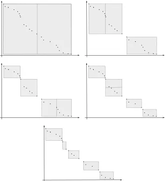
Figure 1 demonstrates the steps of the algorithm and highlights the results obtained by its use. Consider the set of 24 points in the bi-objective space depicted in the top left panel of Figure 1. Suppose that the purpose is to partition this set into m = 5 subsets. The gray rectangle represents the region in the objective space that contains the solutions of the set. According to Eq. (3), the diameter of the given set is the length of the horizontal side of the rectangle. Therefore, the first partition is made by vertical incision (indicated by the vertical line in the middle of the rectangle). The results of this partition are depicted in the top right panel of Figure 1. The left subset in this panel has the greatest diameter (in horizontal direction). Therefore, the next partition is made on this subset by vertical incision. The results of this partition are depicted in the middle left panel of Figure 1. The other two panels of Figure 1 depict the results of the next two iterations of Algorithm 1. Note that the results of the partitioning are different than the results of using a common grid in the original space. With a common grid, an initial interval in every dimension is divided into equal sections, resulting in the division of the hyperbox into smaller hypberboxes of equal space. Since the original set A does not necessarily ‘cover’ the entire space, each hyperbox in the grid might or might not contain a member of A. Hence, there is no way to predict which resulting grid will have the desired number of occupied boxes. In addition, there are certain limitations on the number of hyperboxes in the grid. For example, in a two-dimensional grid it is possible to create

m ={1,2,4,6,9,12, . . .} boxes, while only a number of m=n2_{, when n is}

a positive integer, will produce an even grid. With PSA, only the occupied space (marked as the gray rectangles in Figure 1) is considered. When a set

Ai is partitioned into two subsets Ai₁ and Ai₂, the space considered from

now on is given only by the two hyperboxes circumscribingAi₁ andAi₂. The

rest of the space inAi is discarded. Every partition increases the number of

subsets by one, and therefore any desired number of subsets can be created.

2.2 Selection of a Representative Subset

Once the set A has been partitioned into the m subsets A1, . . . , Am, the

‘most suitable’ element from each subset must then be chosen in order to obtain a subsetA(r)ofAthat containsmelements. This is of course problem

dependent. Since this study aims for high diversity of the chosen elements, the following heuristic is suggested (denoted as center point selection): From each setAi choose the member which is closest (in Euclidean metric) to the

center of the hyperrectangle circumscribingAi. If there exist more than one

member closest to the center, one of them is chosen randomly.

Fig. 1 Partitioning of 24 elements in bi-objective space intom= 5 subsets (indicated by the gray boxes). (borrowed from [22])

to the center is circled (a random member is circled in the subset with only two members). The representative setA(r)={a1, a2, a3, a4, a5} is the set of

all circled points.

Fig. 2 Selection of a representative subset A(r) out of A using center point selection

(borrowed from [22])

the subset of the circles from Figure 3(b) has the largest dissimilarity and therefore is partitioned (over f1). At the next partition the subset of gray

stars is partitioned over f1 to form the four subsets shown in Figure 3(d).

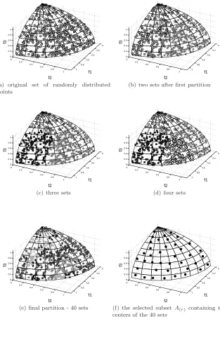
The final stage of Algorithm 1 is shown in Figure 3(e). The subset shown in Figure 3(f) is obtained by selecting the point closest to the center of each of the 40 subsets. Figure 3(a) clearly shows that the distribution of the points in the original set is not uniform. Nevertheless, PSA managed to select a subset of fairly evenly distributed points from it.

2.3 NSGA-II-PSA

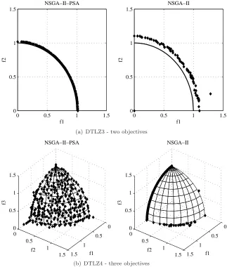
NSGA-II-PSA was introduced in [22] as an improvement of the well-known NSGA-II [13] by a straightforward integration of the PSA into it. The algo-rithm differs from its base EMOA in the selection of the elite population, and in the crowding measure assignment; both of which are conducted by using the PSA. The approximated sets obtained by NSGA-II-PSA were better then those obtained by NSGA-II in terms of both spread and convergence. Figure 4 depicts some of the comparative results between NSGA-II and NSGA-II-PSA, conducted in [22].

3 A New EMOA with PSA as a Diversity Preservation

Operator

candi-0 0.2 0.4 0.6 0.8 1 0 0.2 0.4 0.6 0.8 1 0 0.2 0.4 0.6 0.8 1 f1 f2 f3

(a) original set of randomly distributed points 0 0.2 0.4 0.6 0.8 1 0 0.2 0.4 0.6 0.8 1 0 0.2 0.4 0.6 0.8 1 f1 f2 f3

(b) two sets after first partition

0 0.2 0.4 0.6 0.8 1 0 0.2 0.4 0.6 0.8 1 0 0.2 0.4 0.6 0.8 1 f1 f2 f3

(c) three sets

0 0.2 0.4 0.6 0.8 1 0 0.2 0.4 0.6 0.8 1 0 0.2 0.4 0.6 0.8 1 f1 f2 f3

(d) four sets

0 0.2 0.4 0.6 0.8 1 0 0.2 0.4 0.6 0.8 1 0 0.2 0.4 0.6 0.8 1 f1 f2 f3

(e) final partition - 40 sets

0 0.2 0.4 0.6 0.8 1 0 0.2 0.4 0.6 0.8 1 0 0.2 0.4 0.6 0.8 1 f1 f2 f3

(f) the selected subsetA(r) containing the

centers of the 40 sets

Fig. 3 Demonstration of PSA in a three-dimensional space: Selection of a representative

0 0.5 1 1.5 0

0.5 1 1.5

f1

f2

NSGA−II−PSA

0 0.5 1 1.5

0 0.5 1 1.5

f1

f2

NSGA−II

(a) DTLZ3 - two objectives

0

0.5

1

1.5 0

0.5 1

1.5 0

0.5 1 1.5

f1 NSGA−II−PSA

f2

f3

0

0.5

1

1.5 0

0.5 1

1.5 0

0.5 1 1.5

f1 NSGA−II

f2

f3

(b) DTLZ4 - three objectives

Fig. 4 The final approximated set obtained by NSGA-II-PSA and NSGA-II after 25,000

function evaluations for two objectives and 75,000 for three objectives. (borrowed from [22])

population:Pt+1=PtP+1∪PtD+1. The proportion between the sizes of the two

sets is controlled by the proximity factorαin the following manner:|PP t+1|=

αN , |PD

t+1| = (1−α)N , where N =|Pt+1|. The tournament selection for

each population is also conducted according to its aim: Members from PP t+1

are compared, as in NSGA-II-PSA, according to proximity and secondly, as a tiebreaker, according to diversity. Members from PD

t+1 are compared

according to diversity, and secondly according to proximity. After selection, the members of both sets are combined, and crossover and mutation are applied to form the next offspring population Qt+1. This procedure might

produce offspring that are better both in proximity and in diversity.

By selecting according to remoteness, a highly dominated solution can be graded with a high fitness. This approach is not intuitive, and indeed, there are no methods known to the authors that give high priority to domi-nated solutions. Therefore, a justification of that novel approach is given here through an example. Consider the following MOP, which is a slight variation1

of DTLZ4 for two objectives [24]:

Minimize f1(x) =r(x) cos (θ(x))

Minimize f2(x) =r(x) sin (θ(x))

where x= [x1, . . . , x7]T , 0≤xi≤1

θ(x) =π

2 (1−2|x1−0.5|)

100

r(x) = 1 +

7

X

i=2

(xi−0.5)2

(4)

Proximity to the true Pareto front is defined by the value ofr(x), and the location along the Pareto front is defined by the value of θ(x). The Pareto optimal set corresponds to r= 1, i.e.,xi= 0.5 for alli= 2, . . . ,7, and to all

the values ofθ between 0 and π/2. The mapping from x1 to θ, as depicted

in Figure 5(b), results inθ values close to zero for 98% of thex1 values. All

other values ofθcorrespond to 0.49< x1<0.51. Figure 5 depicts a random

population of 500 solutions. Only two solutions of this population have θ

value greater than 0.1 radian. Both of them are dominated by most of the other solutions. An algorithm that favours non-dominated solutions will skip these two solutions, and their genetic information (i.e.,x1close to 0.5), which

is important to spread the approximated set along the Pareto front, will be lost.

1 _{The difference of the problem in Eq. (4) from DTLZ4 is that the peak ofθ(x} 1) is at x1 = 0.5 rather than atx1= 1. It moves the area of interest away from the limits of the

0 0.5 1 1.5 2 0

0.5 1 1.5 2

f

1

f

2

(a) Objective values of random 500 solu-tions. The real Pareto front is marked with a bold line.

0 0.2 0.4 0.6 0.8 1

0 0.2 0.4 0.6 0.8 1 1.2 1.4 1.6

x

1

θ θ(x1)

random points

(b) The mapping fromx1 toθ

Fig. 5 A random initial population of 500 solutions for the MOP of Eq. 4.

The algorithm of DPGA is presented in Algorithm 2. A discussion about the setting of α(Step 4) appears in Section 3.3. Steps 5–7 are explained in Section 3.1. Steps 8–9 are explained in Section 3.2.

Algorithm 2DPGA - Diversity Preservation Genetic Algorithm

1: R1←Generate a random set of solutions of size 2N

2: t←1

3: whileStopping criteria not metdo

4: Setα

5: PP

t+1←PreserveαN solutions fromRtbased on non-dominance

6: R∗

t ←Rt\PtP+1

7: PD

t+1←Preserve (1−α)N solutions fromR∗t based on diversity.

8: QP

t+1←SP(PtP+1)

9: QD

t+1←SD(PtD+1)

10: Q∗

t+1←QPt+1∪QDt+1

11: Q∗∗

t+1←CrossOver(Q∗t+1)

12: Qt+1←M utation(Q∗∗t+1)

13: Rt+1←PtP+1∪PtD+1∪Qt+1

14: t←t+ 1

3.1 Elite Preservation in DPGA

At each generation DPGA preservesN members in the elite (parent) popu-lation Pt+1, from the current populationRt of size 2N. This is done in two

using the PSA, and including one member of each subset inPD

t+1. During the

elite preservation stage every member i in Pt+1 is given a proximity

mea-sureirank and a diversity measureidiversity. The criteria for these measures

are different for the members ofPP

t+1 andPtD+1. The exact procedure of the

elite preservation and the fitness assignment is described in Algorithm 3. The procedure is illustrated in Figure 6.

Algorithm 3Elite Preservation in DPGA

PP

t+1←PreserveαN solutions fromRtaccording to NSGA-II-PSA

assign proximity and diversity measures to the solutions inPP

t+1according to

NSGA-II-PSA.

R∗

t ←Rt\PtP+1

PartitionR∗

t with PSA to (1−α)N subsetsD=

D1, . . . , D(1−α)N

PD t+1← ∅

foreachDi∈ Ddo

Di,nd= nondominated solutions ofDi

di←center point selection fromDi,nd

Assign a diversity measure todiequal to|Di,nd|

PD t+1←

PD t+1,di

SortPD

t+1to ranks of non-dominance, and assign a proximity measure to each member

according to its rank

Pt+1←PtP+1∪PtD+1

3.2 Selection in DPGA

As NSGA-II, DPGA also uses a binary tournament selection from Pt+1 to

form the children populationQt+1. The comparison between two candidate

parents is done according to the proximity and diversity measures assigned to each member inPt+1. The difference from NSGA-II is that two tournaments

are done in parallel; one for the population ofPP

t+1, and another forPtD+1.

The diversity oriented selection operatorSD, applied onPtD+1, is described

in Algorithm 4. The proximity oriented selection operator SP, which is in

fact the crowded comparison operator ≺n of NSGA-II, is the same as SD,

except for Condition 4, that in the case of SP gives the first priority to the

0 0.5 1 1.5 0

0.5 1 1.5

f1 f2

R

t *

P

t+1 P

(a)

0 0.5 1 1.5

0 0.5 1 1.5

D₁

D

2

D

3

f1

f2

P

t+1 P

D

i,nd

P

t+1 D

(b)

Fig. 6 Elite selection in DPGA. The 12 members preserved for proximity from the 30

members of the previous generation’s population are marked with squares in (a). Preserva-tion of 3 addiPreserva-tional members for diversity is demonstarted in (b). The remaining members are divided into 3 sets D1,D2 andD3. The non dominated members of each setDi,nd

are marked with small diamonds. The central members of eachDi,nd, marked with large

diamonds, are preserved inPD t+1

Algorithm 4SD - Diversity Oriented Selection Operator

1: QD t+1← ∅

2: fork= 1 to (1−α)Ndo

3: Randomly select membersiandjfromPD t+1

4: if(idiversity< jdiversity)or((idiversity=jdiversity)and(irank< jrank))then

5: QD

t+1←QDt+1∪ {i}

6: else

7: QD

t+1←QDt+1∪ {j}

3.3 Sensitivity to Parameters

solu-DPGA consists of two stages; at the first stage a constant value of α ∈

(0,1) is set; at the second stage the selection is done as in NSGA-II-PSA (it can be conducted by simply set α to one). This heuristic requires two a-priory decisions – the value of α at the first stage, and when to switch from the first to the second stage. The second decision can be described through a parameterµ– the portion of the generations in which the selection is done according to DPGA. The proper values of α and µ are problem dependent, and it is out of the authors’ ability at the moment to suggest a generic way to determine them. An analysis of the performance of DPGA for one benchmark, with different values of these parameters, is given in Section 4. The conclusions on the parameters setting for this benchmark can be implemented as a starting point for other problems.

Other heuristics, such as a gradual increase ofα, or setting αas a func-tion of the generafunc-tion count, can lead to better performance, but may be associated with more parameters. Probably, the proper way is to change α

according to the progress of the global search. Meaning, to decrease it when the elite population loses its diversity, and to increase it otherwise. This should be done automatically within the evolutionary algorithm.

4 Simulations for DPGA

In this section, the proposed DPGA is evaluated and the sensitivity of the parameters α and µ is studied. The algorithm is analyzed on the DTLZ4 benchmark with 3 objectives. This benchmark is used, since it poses a spe-cial challenge in spreading the approximated set. This is exactly the kind of problems the DPGA should be used for. The conclusions on the parameters setting for this problem can be implemented as a starting point for other problems. The approximated sets are evaluated by the hypervolume measure (HV) [10].

First, the algorithm is tested for different values ofαandµ. The values of

α={0,0.15,0.3,0.45,0.6,0.75,0.9,1} andµ ={0,0.1,0.2,0.3,0.4,0.5} were examined for all possible combinations. Fifty independent runs were carried out for each setting. For the sake of proper comparison, all combinations of parameter setting ran on the same fifty initial populations. The parameter setting of α= 1 orµ= 0 is the NSGA-II-PSA algorithm without the modi-fications of DPGA. Therefore, these settings are evaluated only once on the test set, and the corresponding results are referred to as ”NSGA-II-PSA”.

ref-erence in this test. Each algorithm solves the problem for 100 times with the same initial population which caused in the worst performances in the previous simulations.

4.1 Experimental Setup

Both algorithms are given real-valued decision variables. They use the sim-ulated binary crossover (SBX) operator and polynomial mutation [25], with distribution indices of ηc = 20 and ηm= 20 respectively. A crossover

prob-ability of pc = 1 and a mutation probability of pm = 1/3 are used. The

population size is set to 300, and the number of generations to 250.

4.2 Results of DPGA with Various Parameter Settings

The HV values of the final results in all the tests varied between 7.325 and 7.435. Approximated sets with values larger than 7.4 include at least some solutions on the surface of the sphere of the Pareto front. Sets with lower HV values consist of solutions on the f1−f2 plane andf1−f3 plane only.

Results of that kind are considered as a failure of the algorithm to spread the approximated set along the Pareto front. Figure 7 depicts a boxplot of the statistic results of the NSGA-II-PSA (α= 1,µ= 0) and one parameter setting (α= 0.15, µ = 0.4), as well as three approximated fronts and their HV values. The results in Figure 7(b) are considered as a failure. Those in Figure 7(c) are quite poor, and the results in Figure 7(d) are considered as good results. The boxplot of NSGA-II-PSA in Figure 7(a) shows the failures of the algorithm as outliers. The boxplots in Figure 7(a) indicate that there is no statistically significant difference in location of the HV values of NSGA-II-PSA and DPGA. On the other hand, DPGA with the above parameter setting is much more consistent regarding to different initial populations, and has no failures in spreading the approximated front. NSGA-II-PSA has 11 failures out of 50.

The results of the statistic evaluation of all the combinations of α and

7.32 7.34 7.36 7.38 7.4 7.42 7.44 NSGA−II−PSA DPGA HV

(a) Boxplots for NSGA-II-PSA and for DPGA withα= 0.15 andµ= 0.4

0 0.5 1 1.5 0 0.5 1 1.5 0 0.5 1 1.5 f1 f2 f3

(b)HV = 7.3254

0 0.5 1 1.5 0 0.5 1 1.5 0 0.5 1 1.5 f1 f2 f3

(c) HV = 7.4103

0 0.5 1 1.5 0 0.5 1 1.5 0 0.5 1 1.5 f1 f2 f3

(d)HV = 7.4348

Fig. 7 HV values of 50 tests for NSGA-II-PSA and DPGA, and examples for the HV

measure associated with three approximated Pareto fronts. HV values that are less than 7.4 are considered as a failure to spread the approximated set along the Pareto front (e.g., the outliers of NSGA-II-PSA, marked as red crosses, and the results in Figure 7(b)).

reduces the chance of a failure for most parameter settings (especially for

α <0.5 andµ≥0.2); (c) for this benchmark, the mean performance is more affected from the number of failures, and therefore, DPGA has a better mean HV than NSGA-II-PSA for most of the parameter settings.

0 0.2 0.4 0.6 0.8 1 7.43 7.431 7.432 7.433 7.434 7.435 α

Best HV NSGA−II−PSA µ = 0.1

µ = 0.2

µ = 0.3

µ = 0.4

µ = 0.5

(a)

0 0.2 0.4 0.6 0.8 1

7.4265 7.427 7.4275 7.428 7.4285 7.429 7.4295 7.43 7.4305 7.431 α Median HV NSGA−II−PSA

µ = 0.1

µ = 0.2

µ = 0.3

µ = 0.4

µ = 0.5

(b)

0 0.2 0.4 0.6 0.8 1

7.4 7.405 7.41 7.415 7.42 7.425 7.43 α Mean HV NSGA−II−PSA

µ = 0.1

µ = 0.2

µ = 0.3

µ = 0.4

µ = 0.5

(c)

0 0.2 0.4 0.6 0.8 1

0 0.05 0.1 0.15 0.2 0.25 α

Percentage of failures

NSGA−II−PSA

µ = 0.1

µ = 0.2

µ = 0.3

µ = 0.4

µ = 0.5

(d)

Fig. 8 Statistic results of 50 tests for NSGA-II-PSA and for DPGA with different values

ofαandµ.

To choose the best parameter setting of DPGA for the DTLZ4 benchmark according to these results, the main objective should be the reduction of failures. In general, the percentage of failures decreases with the increase of

µand the decrease ofα. Bothµ= 0.4 andµ= 0.5 satisfy this demand. Due to the inevitable tradeoff between proximity and diversity, the performance should be considered as well, reflected by the mean, median and best HV. Considering all the above, the best parameter setting for this benchmark is

α= 0.15, µ= 0.4. It had no failures, and has the best performance over all the other settings with no failures.

4.3 Poor Initial Population

popu-µ, and to NSGA-II-PSA, and is solved by each algorithm for 100 times.

0 20 40 60 80 100

7.3 7.35 7.4 7.45 7.5

test no.

HV

(a) NSGA-II-PSA

0 20 40 60 80 100

7.3 7.35 7.4 7.45 7.5

test no.

HV

(b) DPGA

Fig. 9 Results of 100 tests with a poor initial population. For clarity, the results are sorted

according to performance.

The HV values of the obtained approximated fronts are depicted in Fig-ure 9. The advantage of DPGA over II-PSA is clear. While NSGA-II-PSA has failed 45 times in finding solutions on the surface of the sphere, DPGA has only failed 3 times. The HV of the successful results are quite the same for both algorithms.

5 Using PSA for Hausdorff Approximations of the

Pareto Front

In this section, a first attempt is made to show that PSA can be used suc-cessfully within EMOAs to compute Hausdorff approximations of the Pareto front. The Hausdorff distance dH (e.g., [26]) prefers, roughly speaking,

ap-proximationsA⊂R

n _{such that its images are located equally spaced along}

the Pareto front. Hence,dH can be viewed as a performance indicator that

is closely related to the terms spread andconvergence as used in the EMO community. PSA is integrated into NSGAII-I [27] to produce two new al-gorithms: NSGA-II-I-PSA and NSGAII-I-∆p-PSA. Both algorithms use an

approxi-mations2_{than its base EMOA, and NSGAII-I-∆}

p-PSA improved the

perfor-mance in most cases. On models where the Pareto front is connected, both of the new methods cannot compete with∆p-EMOA [28], which is a

special-ized algorithm to produce good Hausdorff approximations. NSGA-II-I-PSA, however, is advantageous in cases where the Pareto front is disconnected. We conjecture that this is the merit of PSA that is independent from the geometry of the underlying model. First results for bi-objective problems (i.e., k = 2) are presented here, and considerations of k > 2 and further improvements of the hybrid are kept for future research.

The performance indicator considered in this section, ∆p, is defined as

follows.

Definition 1 (averaged Hausdorff distance ∆p [11]). Letp∈N,

A={a1, . . . , ar} ⊂R

d _{be a candidate set andY ={y}

1, . . . , yr} ⊂R

k _{be its}

image, i.e.,yi=F(ai),i= 1, . . . , r. Further, letP :={p1, . . . , pm} ⊂R

k _be

a discretization of the Pareto front. Then it is

∆p(Y, P) = max



 1

r

r

X

i=1

dist(yi, P)p

!1/p

, 1 m

m

X

i=1

dist(pi, Y)p

!1/p

,

(5) where dist(x, B) := infb∈Bkx−bk denotes the distance between a point x

and a setB.

∆p is a combination of slight variations of the well-known Generational Distance (GD, see [29]) and the Inverted Generational Distance (IGD, see [30]). For p = ∞ the indicator coincides with the Hausdorff distance (i.e.,

∆∞=dH), and hence,∆p can be viewed as an averaged Hausdorff distance.

The NSGA-II-I is a variant of the classical NSGA-II and is based on the conjecture that a sequential update of the crowding distances leads to a more homogeneous distribution of the population than the single determination of the crowding distances of the original NSGA-II. This algorithm is used here as a base EMOA for the new algorithms, that include an additional external archive strategy as indicated in the Figure 10. PSA is being used here for the update of the archive in two variants: (i) it is used as a tool to select the best individuals to be stored in the external archive (NSGA-II-I-PSA), and (ii) PSA is integrated into the procedure of∆p-EMOA [28] that selects the best

individuals to the external archive according to an approximated reference set (NSGAII-I-∆p-PSA). Here, PSA is used as a tool to obtain the reference

set required to compute the distance to the set of interest. The procedure of the external archive strategy using PSA as the tool to select the best individuals in each generation (for NSGA-II-I-PSA) is detailed in Algorithm 6. The procedure where PSA is used to generate the reference set that ∆p

2 _{In fact, we will use theaveraged Hausdorff distance in order to avoid punishments of}

current archive Ai. If the magnitude of N D is greater than the size of the

external archiveNA, then PSA is applied on N Dto obtain a reference front

R of magnitudeNA. This set is further on used to update the archiveAi by

Oi according to the best∆p values with respect to R. Hereby, ∆p-Update

denotes the archiver used in [28] which is given in Algorithm 5, where h(a) is the∆p value of the set of solutionsN D without the solutiona.

Algorithm 5∆p-Update

Require: new solutionoi, archiveAi, reference frontR, archive sizeNA

Ensure: new archiveAi+1

N D= nondominated solutions ofAi∪oi

if|N D|< NA then

for alla∈N Ddo

h(a) =∆p(N D\{a}, R)

a∗_{=argmin{h(a) :a∈N D}}

Ai+1=N D\{a∗}

Fig. 10 General NSGAII-I procedure with an external archive. PSA-Update is being used

Algorithm 6PSA-Update

Require: populationPi, offspringOi, archiveAi, archive sizeNA

Ensure: new archiveAi+1

N D= nondominated solutions ofPi∪Oi∪Ai

if|N D|< NA then

Ai+1=N D

else

Ai+1= PSA(N D,NA)

Algorithm 7∆p-PSA-Update

Require: populationPi, offspringOi, archiveAi, archive sizeNA

Ensure: new archiveAi+1

N D= nondominated solutions ofPi∪Oi∪Ai

if|N D|< NA then

Ai+1=N D

else

R= PSA(N D,NA)

Ai+1=∅

for allo∈Oido

Ai+1=∆p-Update(o,Ai,R)

To test the new algorithms, they are first evaluated on four test problems with different characteristics: (i) the bi-objective sphere model [28] that has a convex Pareto front, (ii) DTLZ3 [24] that has a concave Pareto front, (iii) the Dent problem [31] that has a convex-concave front, and (iv) ZDT3 [32] where the Pareto front is disconnected. The number of decision variables and their ranges are specified as recommended in literature, for the bi-objective sphere model 0≤xi ≤1 (i= 1,2), for the DTLZ3 0≤xi≤1 (i= 1, ...,10),

for the Dent −1.5 ≤ xi ≤ 1.5 (i = 1,2) and for the ZDT3 0 ≤ xi ≤ 1

(i= 1, ...,20). Twenty independent test runs are made, each with a budget of 50,000 function calls, a population size equal to 100 and an archive size

NA equal to 100. All algorithms have been implemented in jMetal [33]. The

simulated binary crossover operator is parameterized by a component-wise probability equal to 0.9 and a distribution index equal to 20. Polynomial mutation is applied using a mutation probability equal to 1/d (d= number of decision variables) and the distribution index equal to 20. Table 1 shows the obtained numerical results for the∆p indicator wherep= 1, and Figure

11 shows boxplots of the∆pvalues at the final generation. The∆p indicator

is calculated based on fixed reference fronts referred to as benchmark fronts in the following. Ideal benchmark fronts are composed of the set ofmsolutions with minimum ∆p value with respect to the true Pareto front, where m

denotes the population size of the EMOA. As the true Pareto fronts of the test problems are known in this study, these fronts are composed bymwell distributed points along the true Pareto front (i.e. the set of mpoints with optimal PL-metric as it is defined in [28]). It can be seen that the∆p-EMOA

confirmed by this means, regarding the comparison to the∆p-EMOA.

Table 1 Averaged∆1 values for test problems with different characteristics.

Sphere model DTLZ3 Dent ZDT3

NSGAII-I 0.00503875 0.00638702 0.01618773 0.00591195

NSGAII-I-PSA 0.00460146 0.00621689 0.01501212 0.00527150

NSGAII-I-∆p-PSA 0.00473097 0.00680468 0.01539346 0.00552639

∆p-EMOA 0.00003729 0.00495835 0.00067532 0.00777191

Fig. 11 Boxplots of∆p-values at final generation.

Kursawe, Poloni, Schaffer, and ZDT3. The setting of the experiments is the same as for the previous ones. The number of decision variables and their ranges are as follows: For the Kursawe −5 ≤ xi ≤ 5 (i = 1,2,3), for the

Poloni (−1∗π)≤xi ≤π (i= 1,2), for the Schaffer−5≤ xi ≤10 (i= 1)

and for the ZDT3 0 ≤ xi ≤ 1 (i = 1, ...,20). Table 2 shows the obtained

results, and Figures 12 – 15 show the median distance to the Pareto front in terms of ∆1 on the ordinate and the number of function evaluations on

the abscissa. NSGA-II-I-PSA wins the competition on all four models which is most probably due to PSA that is independent of the geometry of the problem.∆p-EMOA prefers connected Pareto fronts since the reference front

needed for the∆p archiver is built on the assumption that the Pareto front is

connected [28]. Such an assumption is not made in PSA. To take into account the stochastic nature of the EMOA and to show the performance differences are significant, Figure 16 shows boxplots of the∆p-indicator at the final

gen-eration. The differences in location of the ∆p-values of the NSGAII-I-PSA

compared to the other EMOA are statistically significant, beside for Kursawe. These results are encouraging, however, more investigations are required to obtain a better EMOA aiming for Hausdorff approximations which we leave for future work.

Table 2 Averaged∆1 values for test problems with disconnected fronts.

Kursawe Poloni Schaffer ZDT3

NSGAII-I 0.03966693 0.06964843 0.02621266 0.00592310

NSGAII-I-PSA 0.03470179 0.05784069 0.02189886 0.00515468

NSGAII-I-∆p-PSA 0.03774589 0.06157774 0.02304279 0.00548551

∆p-EMOA 0.03489292 0.08614311 0.03160346 0.00778455

Fig. 13 Median distances to the Pareto front w.r.t.∆pfor Poloni problem.

Fig. 14 Median distances to the Pareto front w.r.t.∆pfor Schaffer problem.

6 Conclusions and Future Work

In this study, the ability of the PSA (Part and Select Algorithm) as a selection mechanism within EMOAs was examined. In one part of the study, PSA was used for elite selection, and in the other it was used as an archiving tool. For both cases, the results of the PSA based algorithms were satisfactory, and they were found to have better performance than their non-PSA equivalents for certain types of optimization problems.

Fig. 15 Median distances to the Pareto front w.r.t.∆pfor ZDT3 problem.

high fitness to solutions that are isolated in the objective space, even if they are dominated, the chances for a failure in spreading the candidate solutions along the Pareto front decrease. As future work the performance of DPGA should be also evaluated for ”regular” optimization problems that do not pose a special challenge to find a diverse set of candidate solutions. Some more comparisons with state-of-the-art EMOAs should be conducted as well. Finally, DPGA can be improved if its related parameterαcould be adjusted automatically. In order to do so, a measure to identify that proximity is over-exploited on the account of diversity, is required. This measure can be used during the progress of the algorithm to decide the appropriate value ofα.

The PSA was found to be also an appropriate archiving tool for Hausdorff approximations inspired EMOAs for special cases. The proposed algorithm NSGAII-I-PSA could not compete with the specialized algorithm for Haus-dorff approximations ∆p-EMOA on models where the Pareto front is

con-nected. However in cases where the Pareto front is disconnected, NSGAII-I-PSA has outperformed the ∆p-EMOA, producing better Hausdorff

approxi-mations to the Pareto front according to the∆pindicator for the four

bench-mark problems selected. The advantage of NSGAII-I-PSA is thanks to that PSA is independent from the geometry of the underlying problem, so the selection of the best solutions with respect to spread and convergence is not affected by the gaps within the Pareto fronts of the problems. We conjec-ture that the consideration of PSA will be particularly advantageous in cases more than three objectives are under consideration. Hence, the extension of the NSGA-II-I-PSA to higher-dimensional problems seems like a promising research direction.

Acknowledgements This research was supported by a Marie Curie International

Re-search Staff Exchange Scheme Fellowship within the 7th European Community Framework Programme.

Oliver Sch¨utze acknowledges support from the CONACyT project no. 128554.

References

1. Coello, C.A.C., Lamont, G.B., Van Veldhuizen, D.A.: Evolutionary algorithms for solving multi-objective problems. Volume 5. Springer (2007)

2. Deb, K.: Multi objective optimization using evolutionary algorithms. John Wiley and Sons (2001)

3. Bosman, P., Thierens, D.: The balance between proximity and diversity in multiobjec-tive evolutionary algorithms. Evolutionary Computation, IEEE Transactions on7(2) (april 2003) 174 – 188

Operational Research197(2) (2009) 701 – 713

5. Abbass, H.: The self-adaptive Pareto differential evolution algorithm. In: Evolutionary Computation, 2002. CEC ’02. Proceedings of the 2002 Congress on. Volume 1. (may 2002) 831 –836

6. Laumanns, M., Rudolph, G., Schwefel, H.: Mutation control and convergence in evo-lutionary multi-object optimization. HT014601767 (2001)

7. Bosman, P.A., Thierens, D.: Multi-objective optimization with diversity preserving mixture-based iterated density estimation evolutionary algorithms. International Jour-nal of Approximate Reasoning31(3) (2002) 259 – 289

8. Li, M., Zheng, J., Xiao, G.: An efficient mufti-objective evolutionary algorithm based on minimum spanning tree. In: Evolutionary Computation, 2008. CEC 2008. (IEEE World Congress on Computational Intelligence). IEEE Congress on. (june 2008) 617 –624

9. Wineberg, M., Oppacher, F.: The underlying similarity of diversity measures used in evolutionary computation. In Cant´u-Paz, E., Foster, J., Deb, K., Davis, L., Roy, R., O’Reilly, U.M., Beyer, H.G., Standish, R., Kendall, G., Wilson, S., Harman, M., Wegener, J., Dasgupta, D., Potter, M., Schultz, A., Dowsland, K., Jonoska, N., Miller, J., eds.: Genetic and Evolutionary Computation — GECCO 2003. Volume 2724 of Lecture Notes in Computer Science. Springer Berlin Heidelberg (2003) 1493–1504 10. Zitzler, E.: Evolutionary Algorithms for Multiobjective Optimization: Methods and

Applications. PhD thesis, Swiss Federal Institute of Technology Zurich (1999) 11. Sch¨utze, O., Esquivel, X., Lara, A., Coello, C.: Using the averaged Hausdorff distance

as a performance measure in evolutionary multiobjective optimization. Evolutionary Computation, IEEE Transactions on16(4) (aug. 2012) 504 –522

12. Horn, J., Nafpliotis, N., Goldberg, D.: A niched Pareto genetic algorithm for multiob-jective optimization. In: Evolutionary Computation, 1994. IEEE World Congress on Computational Intelligence., Proceedings of the First IEEE Conference on. (jun 1994) 82 –87 vol.1

13. Deb, K., Pratap, A., Agarwal, S., Meyarivan, T.: A fast and elitist multiobjective genetic algorithm: NSGA-II. Evolutionary Computation, IEEE Transactions on6(2) (apr 2002) 182 –197

14. Xiaoning, S., Min, Z., Tao, L.: A multi-objective optimization evolutionary algorithm addressing diversity maintenance. In: Computational Sciences and Optimization, 2009. CSO 2009. International Joint Conference on. Volume 1. (april 2009) 524 –527 15. Zitzler, E., Laumanns, M., Thiele, L.: SPEA2: Improving the strength Pareto

evolu-tionary algorithm for multiobjective optimization. In Giannakoglou, K., et al., eds.: Evolutionary Methods for Design, Optimisation and Control with Application to In-dustrial Problems (EUROGEN 2001), International Center for Numerical Methods in Engineering (CIMNE) (2002) 95–100

16. Zhang, Q., Li, H.: MOEA/D: A multiobjective evolutionary algorithm based on de-composition. Evolutionary Computation, IEEE Transactions on11(6) (dec. 2007) 712 –731

17. Zuiani, F., Vasile, M.: Multi agent collaborative search based on Tchebycheff decom-position. Computational Optimization and Applications (March 2013) 1–20

18. Batista, L., Campelo, F., Guimar˜aes, F., Ram´ırez, J.: Pareto cone epsilon-dominance: Improving convergence and diversity in multiobjective evolutionary algorithms. In Takahashi, R., Deb, K., Wanner, E., Greco, S., eds.: Evolutionary Multi-Criterion Optimization. Volume 6576 of Lecture Notes in Computer Science. Springer Berlin Heidelberg (2011) 76–90

impact on the performance of moeas. In Obayashi, S., Deb, K., Poloni, C., Hiroyasu, T., Murata, T., eds.: Evolutionary Multi-Criterion Optimization. Volume 4403 of Lecture Notes in Computer Science. Springer Berlin Heidelberg (2007) 5–20

22. Salomon, S., Avigad, G., Goldvard, A., Sch¨utze, O.: PSA – a new scalable space partition based selection algorithm for MOEAs. In Sch¨utze, O., ed.: EVOLVE - A Bridge between Probability, Set Oriented Numerics, and Evolutionary Computation II. Volume 175 of Advances in Intelligent Systems and Computing. Springer Berlin Heidelberg (2013) 137–151

23. Avigad, G., Matalon Eisenstadt, E., Salomon, S., Gadelha Guimar, F.: Evolution of contours for topology optimization. In Sch¨utze, O., ed.: EVOLVE - A Bridge between Probability, Set Oriented Numerics, and Evolutionary Computation II. Volume 175 of Advances in Intelligent Systems and Computing. Springer Berlin Heidelberg (2013) 397–412

24. Deb, K., Thiele, L., Laumanns, M., Zitzler, E.: Scalable multi-objective optimization test problems. In: Evolutionary Computation, 2002. CEC ’02. Proceedings of the 2002 Congress on. Volume 1. (may 2002) 825 –830

25. Deb, K., Agrawal, R.: Simulated binary crossover for continuous search space. Complex systems9(2) (1995) 115–148

26. Heinonen, J.: Lectures on Analysis on Metric Spaces. Springer New York (2001) 27. Kukkonen, S., Deb, K.: Improved pruning of non-dominated solutions based on

crowd-ing distance for bi-objectve optimization problems. In: Proceedcrowd-ings of the 2006 IEEE Congress on Evolutionary Computation, IEEE Press (2005) 1179–1186

28. Gerstl, K., Rudolph, G., Sch¨utze, O., Trautmann, H.: Finding evenly spaced fronts for multiobjective control via averaging Hausdorff-measure. In: Int’l. Proc. Conference on Electrical Engineering, Computing Science and Automatic Control (CCE 2011). (2011) 975–980

29. Van Veldhuizen, D.A.: Multiobjective Evolutionary Algorithms: Classifications, Anal-yses, and New Innovations. PhD thesis, Department of Electrical and Computer En-gineering. Graduate School of EnEn-gineering. Air Force Institute of Technology 30. Coello, C.A.C., Cort´es, N.C.: Solving multiobjective optimization problems using an

artificial immune system. Genetic Programming and Evolvable Machines6(2) (June 2005) 163–190

31. Sch¨utze, O., Laumanns, L., Tantar, E., Coello, C.A.C., Talbi, E.G.: Computing gap free Pareto front approximations with stochastic search algorithms. Evolutionary Com-putation18(1) (2010) 65–96

32. Zitzler, E., Deb, K., Thiele, L.: Comparison of multiobjective evolutionary algorithms: Empirical results. Evol. Comput.8(2) (June 2000) 173–195