Angles-only navigation of a formation in the proximity of a binary system

(1)

Angles-Only Navigation of a Formation in the Proximity of a

Binary System

Francesco Torre∗, Romain Serra†, Stuart Grey‡and Massimiliano Vasile§

University of Strathclyde, Glasgow, G1 1XJ, United Kingdom

This paper will focus on the navigation and station keeping of one or more spacecraft around the dynamic equivalent of the Lagrange point L4 of a binary asteroid system. This location can be conveniently used by a spacecraft equipped with a small scale laser to demonstrate laser ablation as a viable asteroid deflection technology and to extract and analyse surface and subsurface material. This paper proposes an approach using optical navigation only and exploiting the knowledge of the dynamics of the secondary asteroid around the primary. Each spacecraft is equipped with only a camera, a good attitude determination and control system and an inter-satellite link that allows sharing information with other spacecraft in the formation and provides a complete spacecraft-to-spacecraft position vector.

Two scenarios will be considered in this study: one in which a single spacecraft uses only information from a camera observing both the primary and the secondary asteroid, in the other, a small formation of spacecraft autonomously navigates using only cameras and an inter-satellite link. Measurements and dynamics are processed in a form of Unscented H-infinity Filter that can effectively estimate the state of the system and allows maintaining the formation at L4.

I. Nomenclature

A = primary asteroid

Ai = cross sectional area of spacecrafti

ai = semi-axis along thex-axis of the body fixed frame of bodyi

aSR Pi = acceleration vector due to the solar radiation pressure (SRP) on spacecrafti

B = secondary asteroid

bi = semi-axis along they-axis of the body fixed frame of bodyi

C = camera coordinate system

Ci j = spherical harmonics coefficient of degreeiand orderj

CRi = reflectivity coefficient of spacecrafti

ci = semi-axis along thez-axis of the body fixed frame of bodyi

dr = distance between two spacecraft

f = generic function for dynamics fC = focal length of the camera

h = generic measurement function Kd = derivative coefficient ofPDcontroller

Kp = proportional coefficient ofPDcontroller

mi = mass of bodyi

Q_{i j} = navigation dynamics weight matrix for test caseiand spacecraft j

Ri j = sensor weight matrix for test caseiand spacecraftj I_R

j = rotation matrix from body-fixed frame of body jto principal reference frame ri = position vector of bodyiin the principal reference frame

∗_{PhD student, Aerospace Centre of Excellence, Department of Mechanical and Aerospace Engineering, AIAA Student Member}

†_{Research Associate, Aerospace Centre of Excellence, Department of Mechanical and Aerospace Engineering, James Weir Building}

‡_{Teaching Fellow, Aerospace Centre of Excellence, Department of Mechanical and Aerospace Engineering, James Weir Building, Glasgow, G1}

1XJ

§_{Professor, Aerospace Centre of Excellence, Department of Mechanical and Aerospace Engineering, James Weir Building, Glasgow, G1 1XJ,}

(2)

rij = relative position vector from bodyitojin the principal reference frame

SSR P = solar radiation pressure at 1 AU

SC = spacecraft body-fixed coordinate system

t = time

Ui j = gravitational potential of degreeiand orderj ui = control vector of spacecrafti

VC = pointing vector from camera to asteroid

X,Y,Z = axes of the principal reference frame ˆ

xi, ˆyi, ˆzi = axes of the body-fixed frame on bodyi

zr = measurement vector of the relative position between the spacecraft αi = complementary angle toπof angleβi

βi = angle between the pointing vector from one s/c to asteroidiand the baseline between asteroid A and B δri j = relative position vector between bodyiand s/cjin the body-fixed frame ofi

ζr = noise vector of the measurementzr µi = gravitational parameter of asteroidi φr = azimuth of the measurement vectorzr ψr = elevation of the measurement vectorzr ωi = angular velocity of asteroidi

II. Introduction

Binary asteroids are systems composed of two asteroids orbiting around their common barycentre. Examples can be found in the Near Earth Object population, such as 2000 DP107, or 65803 Didymos (1996 GT), an Apollo asteroid discovered on April 11, 1996, that is the target of the AIDA mission. Navigating in the proximity of an asteroid is in itself a challenging task due to the complex dynamics induced by the irregular gravity field of the asteroid, the gravity of the Sun and solar radiation pressure. Even more challenging is to navigate a formation of spacecraft, particularly with heterogeneous sensors. Recent work by one of the authors demonstrated the possibility to autonomously navigate a formation of spacecraft around an asteroid with a distributed fault-tolerant autonomous system [1] [2]. The complexity increases even further in the case of a binary system due the interaction between the primary and the secondary asteroid. Station keeping at the dynamic equivalent of the Lagrange points L4 and L5 of the binary system has been shown to be of particular interest to extract surface and subsurface material with laser ablation [3]. In a previous paper, the authors have already extended to the case of a binary system results on the navigation of single spacecraft and of a formation of spacecraft in the proximity of an asteroid [4]. Such work used a combination of cameras, LIDAR and the relative position vectors between the members of the formation obtained via inter-spacecraft communication (ISC). Nevertheless, the target of the cameras and LIDAR was always the primary asteroid. In this paper the authors exploit the information obtainable by the observation of both the asteroids and the knowledge of the dynamics of the system to navigate using only the cameras and the relative position between the spacecraft.

The dynamical model in the proximity of the binary system includes the gravity of the two asteroids and the Sun as well as solar radiation pressure. Each spacecraft is equipped with a camera and relative position sensor under the assumption of low power and low computational capabilities.

Two scenarios will be considered in this study: one in which a single spacecraft combines the pointing vectors to the two asteroids with the knowledge of the dynamics of the binary system to autonomously navigate. In the other a formation of two spacecraft navigate with the additional information provided by the ISC. It will be shown that the information from the cameras alone allows the formation to autonomously navigate and control their position near L4. In addition, the ISC allows for failure-tolerant navigation as it is able to compensate for degraded performances and even total loss of the camera in one of the members of the formation. Given the non-linear nature of the dynamics the paper will use an Unscented H-infinity Filter.

(3)

III. Dynamic Model

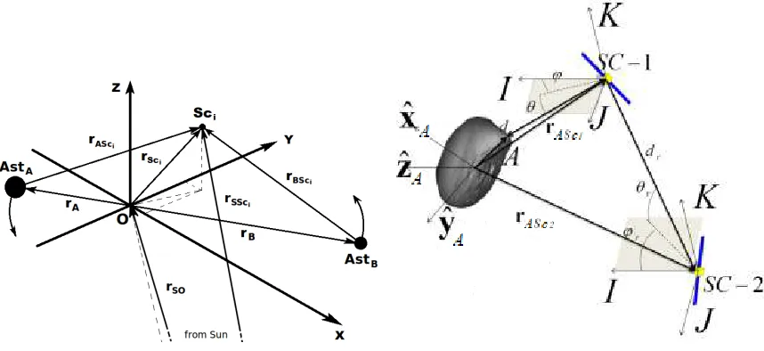
The reference frame chosen for the simulation of the dynamical system is a non-rotating reference frame, centred in the centre of mass of the binary asteroid system (see Fig. 1).

Fig. 1 Reference frame for dynamics and measurement model.

In such a frame, it is assumed that the motion of the asteroids is known and consists of circular coplanar orbits with a rotation period equal to the rotation period of the system. Both of the asteroids can rotate around their respective rotation axes. A assumption is that, while the primary asteroid is considered to be a homogeneous sphere, the secondary asteroid is a homogeneous ellipsoid with semi-axesaB,bBandcB, rotating around the z-axis with angular velocityωB[5].

The gravity field of the secondary asteroid can be expressed as the sum of a spherical field plus a second-degree and second-order field [6]:

U20,22=

µB kδrBScik3

C20

1−3

2cos 2_(θ

B)

+3C22cos2(θB)cos(2ϕB)

(1)

whereδrBSci is the relative position vector between the asteroid B and the spacecraftiin the body-fixed frame B, µBis the asteroid gravitational constant, the harmonic coefficientsC20andC22are a function of the semi-axes:

C20=− 1 10

2cB2−aB2−bB2

C22= 1 20

aB2−bB2

(2)

andθBandϕBare the latitude and longitude angles respectively:

θB=tan−1

zB p

xB2+yB2 !

; ϕB=tan−1

yB

xB

(3)

The conversion from the body-fixed frame to the reference frame is obtained by applying the rotation matrix:

I_R

B=

      

cos(ωBt) −sin(ωBt) 0

sin(ωBt) cos(ωBt) 0

0 0 1

      

(4)

wheretindicates the time. The spacecraft is assumed to be subject to the gravitational force of the Sun, solar radiation pressure and the irregular gravity of the binary system. WithrA,rB,rS andrSci as the position of asteroid

A, asteroid B, the Sun and the i-th spacecraft respectively all in the chosen reference frame, it is possible to define

rASci =rSci−rA,rBSci =rSci −rBandrSSci =rSci−rSas the relative position vectors from the i-th spacecraft to

[image:3.612.90.519.126.323.2]

(4)

Ü rSCi =−

µA krAScik3

rASci − "

µB krBScik3

+I_R B

∂_U

20,22

∂δrBSci

B #

rBSci− µS krSScik3

rSSci+ µS krSk3

rS+aSR Pi +ui (5)

withµS,µAandµBbeing gravity constants of the Sun, asteroid A and B respectively. The quantityaSR Pi represents

the acceleration induced by the solar radiation pressure on spacecrafti, defined as:

aSR Pi =2CRiSSR P

r1AU

rSSci 2

Ai

mSci rSSci

rSSci

(6)

whererSSci is the distance of the i-th spacecraft from the Sun, Ai andmSci are the spacecraft cross sectional area

and mass respectively,CRi is the reflectivity coefficient,SSR Pis the solar radiation pressure at 1 AU andr1AU is one

astronomical unit in km. The vectoru=

ux,uy,uz T

in equation (5) is a control input, which will be defined later in Section V.

If one considers a formation of N spacecraft, the vector equation (5) can be applied to each spacecraft independently and can be re-written in compact form as a system of first order differential equations:

Û

X= f(X,u) (7)

whereX=rSc1, rÛSc1, rSc2, rÛSc2, ... ,rScN, rÛScN T

is the state vector containing the position and velocity of all the spacecraft.

The navigation dynamics are defined in a reference system similar to the one used for the real dynamics. The only difference is that the centre of mass of this system is located in the centre of mass of asteroid A. The reason for this difference is that such a system allows for a relative navigation with respect to the central body. The fictitious force acting on the system due to the motion of asteroid A with respect to the centre of mass of the binary system should be taken into account and the appropriate correction should be applied in the computation of the influence of the Sun. However, in binary systems where the centre of mass is located inside one of the two asteroids, it is possible to neglect these contributions for the sake of simplicity of the equations and consider them as process noises.

IV. Measurement Model

With reference to Figure 1, it is assumed that each spacecraft is provided with the following set of sensors and measurements:

• A camera which provides the pointing unit vector to the centroid of the detected object, expressed in the principal reference frame;

• Inter-spacecraft measurements, which include the relative distance vector between two spacecraft, in Cartesian coordinates.

A good knowledge of the dynamics of the asteroids is assumed when computing the relative position vector between the two asteroids.

A. Camera Model

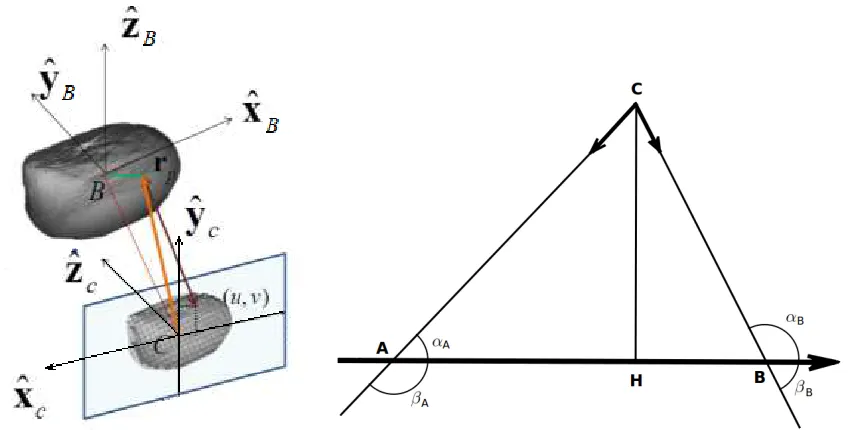
In order to develop the measurement model of the camera, two intermediate reference frames are required as shown in Figure 2:

• Spacecraft coordinate system SC{xscysczsc}: the origin of this frame lies on the centre of mass of the spacecraft,

with the three symmetrical body axes defined as three coordinate axes[7] .

• Camera coordinate system C{xˆCyˆCzˆC}: the centre C is the perspective projection of the camera, with the

zC-axis parallel to the optical axis of the camera and directed to the centre of the asteroid. The image plane is

defined asOC-xC yC.

In this paper, it is assumed that the body reference frame of each spacecraft is aligned with the principal frame and the attitude is known with a level of precision corresponding to that provided by a good star tracker.

(5)

Fig. 2 Projection of asteroid B on the plane of the Pin-Hole camera model and working scheme of the camera-based triangulation method.

conditions. The picture is rotated according to the direction of the Sun, in order to have the light coming from the left of the image plane. Then, an ellipse fitting algorithm is used to compute the coordinates of the centroid of the asteroid in camera coordinates [8]. Once the location of the centroid is known, the pointing vector can be computed as:

VC =

1

kVCk

[xC, yC, fC]T (8)

where fCis the focal length of the camera. Finally, the pointing vector is rotated in the principal reference frame.

B. Inter-spacecraft Measurements

The inter-spacecraft measurement consists of the relative position vector between the two spacecraft in the formation, expressed in the principal reference frame. When a new measurement needs to be computed, the initial relative position vector is composed of the relative distance, local azimuth and elevation, computed in the reference frame of the sensor [9]. The observation equation is given by:

zr =hr

rSci, rScj

=[dr ϕrψr]T +ζr (9)

whereζr= _ζ

dr ζϕr ζψr T

is the measurement noise. The vector is then converted into a Cartesian expression and transformed in to the principal reference frame.

It is important to note that this measurement depends on the knowledge of the positions of the two spacecraft. When a new measurement is simulated, these positions are known exactly; on the other hand, when simulating the measurement during the estimation process, this information needs to be available to each spacecraft. While each spacecraft knows its own state due to the estimation process, the knowledge of the state of another member of the formation is generally unknown. There are two possible solutions: the first is that each spacecraft could estimate the states of all the members of the formation; the second one requires each spacecraft to transmit the estimation of its own state. The first method places significant computational demands on each spacecraft whereas using the second approach makes the simulated measurement depend on thereliabilityof the information provided by the other spacecraft. In this paper the last method is chosen.

C. Camera-based triangulation method

[image:5.612.101.526.75.290.2]

(6)

two asteroids. The segmentABidentifies the relative position vector between the two asteroids; the scalar product between the pointing vectorC Aand the baseline would yield the angleβA, while the one betweenC Band the baseline

would yield βB. This yieldsαA=π−βAandαB=π−βB.

Once the anglesαAandαBand the length of the segment ABare known, the triangle is fully determined. Trivially,

the length of the segmentACcan be obtained as:

AC= sin(αB) sin(αB−αA)

AB (10)

Simply multiplying the value ofACwith the respective pointing vector provides the relative position vector: between the spacecraft atCand the asteroid atAwhen one spacecraft is used; between the spacecraft atAand the asteroid atC in the other case.

It is important to notice that Eq. (10) is undetermined when the triangle degenerates. This happens in two cases: when the three vertices are aligned and whenACandBCare parallel (Cat infinity). In the first case, bothαAandαB

are equal to zero and the ratio of the two sine functions will be undetermined; in the second case,αA=αB, then the

denominator is equal to zero, making the ratio tend to infinity.

V. Control Strategy and State Estimation

The control strategy aims to keep each spacecraft orbiting on a trajectory proximal to the nominal one. Note that this is not an optimal control strategy, but it is sufficient to demonstrate the effect of the navigation algorithm. The control law is given by the simple PD controller:

u=KP © «        x y z       G −        x y z       N ª ® ® ¬

+KD © «        Û x Û y Û z       G −        Û x Û y Û z       N ª ® ® ¬ (11)

where the subscripts G and N stand for guidance and navigation respectively,KPis the proportional coefficient and

KDis the derivative coefficient. If the actual trajectory of the spacecraft is known, the continuous control in Eq. (11)

can be introduced into the full dynamic model in Eq. (5). Here however, the trajectory is estimated by the navigation system with the actual position of the spacecraft never known exactly. The predicted estimation is used by the controller to maintain the relative formation (shown later in Section 5). Once the controller is inserted in the spacecraft dynamic model, one obtains a closed loop problem in which the control is performed together with the estimation, and the filter equations incorporate the action of the controller. During the controlled phases, it is assumed that the asteroid trajectory is precisely known; the state variables to be estimated are only those related to the spacecraft in the formation.

The state estimation process is based on the same UnscentedH∞Filter proposed in [4].

VI. Results

The binary asteroid system chosen as an environment for the simulations is 65803 Didymos, whose parameters are listed in Table 1. The duration of the simulations is set to 5.4 times the orbital period of the secondary asteroid around the primary,TAB, equal to approximately 64.37 hours. For simplicity reasons, the orbital motion of the system around

the Sun has been considered circular; the rotation of the secondary asteroid around the first is assumed on the same plane of the motion of the binary around the Sun. The dimensions, gravitational parameters and angular velocities are chosen according to the current knowledge of the system, with the secondary asteroid being tidally locked with respect to the first one.

Two scenarios will be presented. The first sees one spacecraft keeping its position close to the Lagrangian point L4 of the binary system. The second sees a formation of two spacecraft staying close to L4. In both scenarios, the spacecraft are equipped with one camera assumed to have a resolution of 500x500 pixels, with a field of view of 90 degrees. It is also assumed that the AOCS guarantees a pointing accuracy with standard deviation of 10−3rad and a new measurement is available every 5 minutes.

(7)

[image:7.612.176.434.93.301.2]

Table 1 Orbital and physical parameters for 65803 Didymos

Semi-major axis a 1.6446 AU

Eccentricity e 0.3838

Inclination i 3.4077 deg

RAAN Ω 73.2219 deg

Argument of periapsis ω 319.2516 deg

Orbital period TD 2.11 yr

Distance AB dAB 1.18 km

System rot. period TAB 11.92 h

Grav. param. A µA 3.4908∗10−8km3/s2

Physical dimensions aA,bA,cA 387.5, 387.5, 387.5 m

Rotational velocity ωA 2.26 h

Grav. param. B µB 3.1781∗10−10km3/s2

Physical dimensions aB,bB,cB 81.5, 62.7, 52.2 m

Rotational velocity ωB 11.92 h

measurement and performs a new estimation of its own state. As soon as the new estimation is available, this is transmitted to spacecraft 2. Once spacecraft 2 receives the new information, it calls the relative position sensor to obtain a new measurement to use to perform a new estimation of its state. In the same way, spacecraft 2 transmits the new estimated state to spacecraft 1 and so on. To avoid a continuous and infinite loop of information exchange, aminimum transmission gapis used, i.e. if a new estimation is performed too close to the previous one, its information is not transmitted to the other spacecraft.

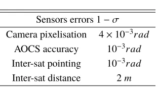
For clarity, all the measurement errors used in the simulations are summarised in Table 2. The mass of each spacecraft is constant and equal to 500 kg, the maximum cross section area is 20 m2and reflectivity coefficientCRis

assumed equal to 1. The initial estimated state is always equal to the real initial state augmented by 20%.

Table 2 Sensors errors

Sensors errors 1−σ

Camera pixelisation 4×10−3r ad AOCS accuracy 10−3_{r ad} Inter-sat pointing 10−3r ad Inter-sat distance 2m

In both the scenarios presented the spacecraft will be required to keep a stable trajectory close to the Lagrangian point L4 of the binary system. This point, due to the irregularities in the gravitational field of the system and the presence of the Sun (gravitational perturbation and radiation pressure) is unstable and the spacecraft is soon swept away if no control is applied. As a final remark, for all the test cases the application of the control is delayed by 2 hours, in order to allow the filters to converge.

For all the test cases, the weight matrices for the navigation dynamics,Qand the measurements,R, are reported in the formQ_{i j} =diag(L,v)meaning thatQ_{i j}is aL×Lmatrix with elements on the diagonal equal tov.

A. Scenario 1: single spacecraft

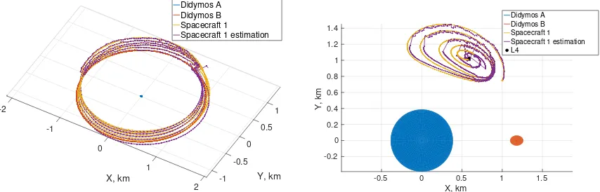
In this scenario, the satellite is positioned at the Lagrangian point L4 of the binary system. Table 3 lists the different test cases analysed for this scenario. A first case, namedCase 1a, is shown where no control is applied. This is to asses the effects of the perturbations on the motion of the spacecraft and the performance of the filter. In this case

Q₁_a = diag(6, 10−12),Rtr iangulation−1a = diag(3, 4×10−4). Fig. 3 shows two different representations of the

[image:7.612.228.384.451.537.2]

(8)

[image:8.612.195.416.94.154.2]

Table 3 Test cases for scenario 1

Case 1a No control Case 1b Default

Case 1c AOCS accuracy 10−2r ad

Case 1d Imperfect knowledge of the binary system

second one in a reference frame centred on the main asteroid and rotating with the binary system. As expected, the spacecraft starts spiralling away from the L4 point due to the perturbations induced by the Sun.

-2 1

0.5 -1

Y, km X, km

0 0

-0.5 1

-1 2

Didymos A Didymos B Spacecraft 1 Spacecraft 1 estimation

-0.5 0 0.5 1 1.5

X, km

-0.2 0 0.2 0.4 0.6 0.8 1 1.2 1.4

Y, km

Didymos A Didymos B Spacecraft 1 Spacecraft 1 estimation L4

Fig. 3 Case 1a: Real and estimated trajectory of the spacecraft in the non-rotating frame (left) and in a frame rotating with the asteroids (right).

0 20 40 60 80

Time, h

10-3 10-2 10-1 100

Error, km

Position estimation error for Spacecraft 1

Error Covariance

0 20 40 60 80

Time, h 10-4

10-3 10-2 10-1 100

Error, m/s

Velocity estimation error for Spacecraft 1

Error Covariance

Fig. 4 Case 1a: estimated position and velocity errors and respective covariance.

[image:8.612.96.523.211.348.2] [image:8.612.119.481.408.593.2]

(9)

the eclipse finishes, new measurements are available and the estimation process resumes, leading to a reduction of the estimation error. From Fig. 4, the average position error increases with time: this is due to the varying position of the spacecraft that drifts further and further away from L4. In fact, the further away the spacecraft is, the smaller the asteroids appear in the image and the less precise the contour extraction and ellipse fitting algorithms become. An additional source of noise is the different shape of the triangle that becomes more skewed.

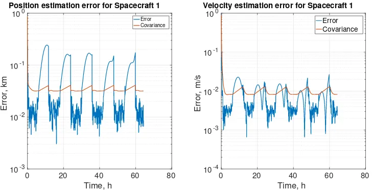
InCase 1b, the spacecraft is tasked to maintain its position as close as possible to L4 and a PD controller is provided. The real and estimated trajectories are depicted in Fig. 5 together with the guidance. Note that, in the rotating frame, the guidance state is just a point that coincides with L4 and the weight matrices used in this case are still

Q₁_b =diag(6, 10−12)andRtr iangulation−1b =diag(3, 4×10−4).

1 -1.5

0.5 -1

-0.5

Y, km 0

X, km 0

0.5 _-0.5

1

-1 1.5

Didymos A Didymos B Spacecraft 1 Spacecraft 1 estimation Spacecraft 1 guidance

-0.5 0 0.5 1 1.5

X, km

-0.2 0 0.2 0.4 0.6 0.8 1 1.2

Y, km

Fig. 5 Case 1b: Real and estimated trajectory of the spacecraft in the non-rotating frame (left) and in a frame rotating with the asteroids (right).

0 20 40 60 80

Time, h

10-3 10-2 10-1 100

Error, km

Error Covariance

0 20 40 60 80

Time, h 10-4

10-3 10-2 10-1 100

Error, m/s

Error Covariance

Fig. 6 Case 1b: estimated position and velocity errors and respective covariance.

[image:9.612.86.513.198.330.2] [image:9.612.119.483.389.575.2]

(10)

about 10 m due to the limited excursions of the spacecraft. Nevertheless, it can be seen that bigger variations in the position error occur at the beginning and end of each eclipse phase. This can be easily attributed again to the poor illumination conditions typical of these phases.

InCase 1c, the pointing accuracy of the AOCS has been degraded to 10−2 _{rad, the navigation dynamics weight} matrix is stillQ1c=diag(6,10−12), while the measurement is nowRtr iangulation−1c=diag(3, 10−3). The trajectories

and estimation errors are in Fig. 7 and Fig. 8. As expected, the steady state errors are bigger than in the previous case, with values generally lower than 60 m for the position error and 2 cm/s for the velocity. Unsurprisingly, the deviations of the real trajectory when no measurements are available are bigger. In fact, the larger estimation errors lead to larger differences in the initial states of the propagation.

0

1 -1.5

0.5 -1

-0.5

Y, km X, km

0 0

0.5 _-0.5

1

1.5 -1

-0.5 0 0.5 1 1.5

X, km

-0.2 0 0.2 0.4 0.6 0.8 1 1.2

Y, km

Fig. 7 Case 1c: Real and estimated trajectory of the spacecraft in the non-rotating frame (left) and in a frame rotating with the asteroids (right).

0 20 40 60 80

Time, h

10-3 10-2 10-1 100

Error, km

Error Covariance

0 20 40 60 80

Time, h 10-4

10-3 10-2 10-1 100

Error, m/s

Error Covariance

Fig. 8 Case 1c: estimated position and velocity errors and respective covariance.

All the results provided so far are based on the assumption that a perfect knowledge of the evolution of the binary system is available. The triangular configuration described in Section IV.C is based on the knowledge of the baseline, that is the relative position vector between the two asteroids. If the knowledge of the system is perfect, this vector is known and the only sources of uncertainty are the orientations of the pointing vectors of the targets of the camera. These depend on the AOCS accuracy and the the number of pixels of the image. However, if the knowledge of the binary system is not perfect, additional uncertainty is generated.

[image:10.612.92.509.204.333.2] [image:10.612.119.483.395.581.2]

(11)

while the navigation dynamics one is set toQ₁_d=diag(3, 10−12), diag(3, 10−11)

.

1 -1.5

0.5 -1

-0.5

Y, km 0

X, km 0

0.5 -0.5

1

-1 1.5

-0.5 0 0.5 1 1.5

X, km

-0.2 0 0.2 0.4 0.6 0.8 1 1.2

Y, km

Fig. 9 Case 1d: Real and estimated trajectory of the spacecraft in the non-rotating frame (left) and in a frame rotating with the asteroids (right) with continuous control applied and imperfect knowledge.

0 20 40 60 80

Time, h

10-2 10-1 100

Error, km

Error Covariance

0 20 40 60 80

Time, h 10-3

10-2 10-1 100

Error, m/s

[image:11.612.87.519.103.235.2]

Error Covariance

Fig. 10 Case 1d: estimated position and velocity errors and respective covariance.

As expected, the performance of the estimation process is affected. From Fig. 9 it is clear that a constant bias in the knowledge of the system produces a corresponding bias in the estimation of the state of the spacecraft. This happens because the knowledge of the dynamical system not only affects the navigational dynamics but also the optical measurement itself. In fact, the orientation of the baseline used during the estimation process is the one that the spacecraftknowsfrom the model provided: an error in this knowledge produces systematically different values of the measurement. From Fig. 10 it is possible to see that, after the transient that follows the end of an eclipse period, the filter manages to provide an estimation with a stable mean position error of about 70 m. This error component, however, cannot be compensated for and increases with the error on the knowledge of the system. It is also important to note that the results shown in this test case are based on the assumption of a constant bias in the information. A bias in the knowledge of the semi-major axis of the system, for example, would produce variable magnitude errors due to the induced difference in the orbital periods that would have a repeatability equal to the synodic period between the real and thebelievedmotion.

B. Scenario 2: two spacecraft

[image:11.612.119.484.294.480.2]

(12)

[image:12.612.196.416.126.187.2]

non-rotating frame as a circular counter-clockwise motion around the primary asteroid, spacecraft 1 is kept around a point 8 deg behind L4, while spacecraft 2 is kept at a point 8 deg ahead of L4. These two locations have a separation of about 300 m. Table 4 contains all the test cases presented for this scenario.

Table 4 Test cases for scenario 2

Case 2a With ISC

Case 2b Pointing accuracy of Sc2 reduced to 10−2 Case 2c No camera for Sc2

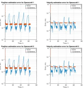
In the first test case,Case 2a, each of the two spacecraft is equipped with a camera and a sensor that computes the relative position. As already described in Section IV.B, the inter-satellite link allows the transmission of the estimated states within the formation. It is assumed again a good knowledge of the dynamics of the system, hence

Q2a =diag(6, 10−12)andRtr iangulation−2a =diag(3, 4×10−4). In addition, the weight matrix of the relative position

sensor is set toRI SC−2a=diag(3, 10−4). The same matrices are used for both the spacecraft. From Fig. 11 it can be

noticed that the trajectories followed by the spacecraft agree with those of the previous scenarios. One difference is at the beginning when the two spacecraft are allowed to drift uncontrolled to allow the filters to converge. An additional difference in this case is that the frequency of the optical measurements is reduced to a new measurement every 10 minutes and spacecraft 2 takes measurements 5 minutes after spacecraft 1. If the frequencies are left at 5 minutes, both the spacecraft would perform the measurement at the same time and then transmit their states to the other one. Then a new estimation would occur immediately for both the spacecraft and a new optical measurement would be available after 5 minutes. This would mean that there would be two consecutive estimation processes very close in time (just the time of the transmission between the spacecraft) and then a waiting phase of roughly 5 minutes. With the reduced frequency and time shift, however, there would be a new estimation every 5 minutes: one time due to the optical measurement, the other time due to the relative position sensor.

Fig. 11 Case 2a: Real and estimated trajectory of the spacecraft in the non-rotating frame (left) and in a frame rotating with the asteroids (right).

The estimation errors are reported in Fig. 12 and one can immediately note that the performances are the same for both the spacecraft, as expected. By comparing them with those obtained inCase 1bit can be seen that the results are quite similar; there might even be a small reduction of the estimation error away from the eclipse phases. On the other hand, it is clear there is a different behaviour of the covariance. What looks like a thick line is in fact a high frequency variation. This happens because of the better accuracy of the relative position sensor with respect to the camera-based one.

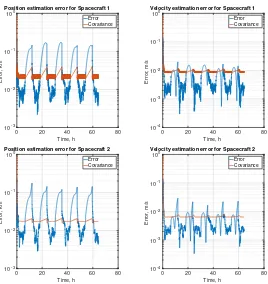
As in Case 1cthe pointing accuracy of spacecraft 2 has been reduced to 10−2 rad to verify whether the ISC manages to compensate. The navigation dynamics weight matrices are left unchanged while the triangulation weight matrix for spacecraft 2 is set toRtr iangulation−2b =diag(3, 10−3)and the relative position one toRtr iangulation−2b=

diag(3, 2×10−4₎_{for both the spacecraft. The trajectories are not reported for this test case because they would not} differ significantly from the ones of the previous test case. The estimation outputs are reported in Fig. 13.

[image:12.612.92.508.402.530.2]

(13)

0 20 40 60 80 Time, h

10-3

10-2

10-1

100

Error, km

Error Covariance

0 20 40 60 80 Time, h

10-4 10-3 10-2 10-1 100

Error, m/s

Error Covariance

0 20 40 60 80

Time, h

10-3

10-2

10-1

100

Error, km

Error Covariance

0 20 40 60 80 Time, h

10-4 10-3 10-2 10-1 100

Error, m/s

[image:13.612.169.437.69.352.2]

Error Covariance

Fig. 12 Case 2a: estimated position and velocity errors and respective covariance.

0 20 40 60 80

Time, h

10-3

10-2

10-1

100

Error, km

Error Covariance

0 20 40 60 80 Time, h

10-4 10-3 10-2 10-1 100

Error, m/s

Error Covariance

0 20 40 60 80

Time, h

10-3

10-2

10-1

100

Error, km

Error Covariance

0 20 40 60 80 Time, h

10-4 10-3 10-2 10-1 100

Error, m/s

Error Covariance

[image:13.612.168.438.384.668.2]

(14)

especially comparing it to the results obtained inCase 1c(Fig. 8) when no ISC was available. This means that the additional information about the relative position between the members of the formation manages to compensate for the lower accuracy of the pointing system. As expected, the amplitude of the oscillations of the covariance for spacecraft 2 is bigger in this case due to the lower reliability of the optical measurement.

Given the satisfactory results of the previous test case it seems reasonable to think whether spacecraft 2 would be able to navigate using the ISC alone. This is tested in test caseCase 2c, where the frequency of the optical measurements for spacecraft 1 is set back to 5 minutes.

0 20 40 60 80

Time, h

10-3

10-2

10-1

100

Error, km

Error Covariance

0 20 40 60 80 Time, h

10-4 10-3 10-2 10-1 100

Error, m/s

Error Covariance

0 20 40 60 80

Time, h

10-3

10-2

10-1

100

Error, km

Error Covariance

0 20 40 60 80 Time, h

10-4 10-3 10-2 10-1 100

Error, m/s

[image:14.612.169.437.165.449.2]

Error Covariance

Fig. 14 Case 2c: estimated position and velocity errors and respective covariance.

From Fig. 14 it is clear that, even without optical measurements, spacecraft 2 is capable of navigating with an average position error of less than 10 m.

VII. Conclusion

The paper presents results on the autonomous navigation of a formation of spacecraft in the proximity of a binary asteroid system. In particular, the formation was specifically trying to maintain the position around L4 in the binary system. It has been shown that a single spacecraft can safely navigate, using optical measurements only and a good knowledge of the motion of the secondary asteroid with respect to the primary, with a position error within 30m.

When a second spacecraft is present, the inter-spacecraft communication is capable of compensating for the degraded accuracy of the pointing system and also to totally compensate the loss of the optical measurements in either one of the spacecraft.

As all of the results presented here depend on the accurate knowledge of the dynamics of the binary system, a perspective would be to set the orbital parameters of the secondary asteroid as part of the quantities estimated with the filter. A more realistic orbital and attitude motion of the binary system could also be simulated by using a mutual gravitational potential. Going even further, the coefficients of the latter could be incorporated in the estimation process itself.

(15)

variables.

References

[1] Vetrisano, M., and Vasile, M., “Autonomous Navigation of a Spacecraft Formation in the Proximity of an Asteroid,”Advances in

Space Research, Vol. 57, No. 8, 2016, pp. 1783, 1804. doi:10.1016/j.asr.2015.07.024.

[2] Vetrisano, M., Colombo, C., and Vasile, M., “Asteroid Rotation and Orbit Control via Laser Ablation,”Advances in Space

Research, Vol. 57, No. 8, 2016, pp. 1762, 1782. doi:10.1016/j.asr.2015.06.035.

[3] Thiry, N., and Vasile, M., “Binary Asteroid Manipulation with Laser Ablation,”HPLA/DE, Santa Fe, 4-6 April 2016, 2016.

[4] Torre, F., Vasile, M., Serra, R., and Grey, S., “Autonomous Navigation of a Formation of Spacecraft in the Proximity of a Binary

Asteroid,”ISTS 2017, Ehime, Japan, 2017.

[5] Scheeres, D. J., “Orbit Mechanics about Asteroids and Comets,”Journal of Guidance, Control and Dynamics, Vol. 35, No. 3,

2012, pp. 987, 997. doi:10.2514/1.57247.

[6] Hu, W., and Scheeres, D. J., “Spacecraft motion about slowly rotating asteroids,”Journal of Guidance, Control and Dynamics,

Vol. 25, No. 4, 2002, pp. 765, 775. doi:10.2514/2.4944.

[7] Li, S., Cui, P. Y., and Cui, H. T., “Vision-aided inertial navigation for pinpoint planetary landing,”Aerospace Science and

Technology, Vol. 11, No. 4, 2007, pp. 499, 506. doi:10.1016/j.ast.2007.04.006.

[8] Christian, J. A., and Lightsey, G. E., “Onboard Image-Processing Algorithm for a Spacecraft Optical Navigation Sensor System,”

Journal of Spacecraft and Rockets, Vol. 49, No. 2, 2012, pp. 337, 352. doi:10.2514/1.A32065.

[9] Alonso, R., Du, J., and Hughes, Y., “Relative Navigation for Formation Flying of Spacecraft,”Proceedings of the Flight