Implementation of Cross-training for Multi-shift Worker Allocation

Rochester Institute of Technology

RIT Scholar Works

Theses Thesis/Dissertation Collections

12-11-2014

Implementation of Cross-training for Multi-shift

Worker Allocation

Aditya Gandhi

Follow this and additional works at:http://scholarworks.rit.edu/theses

This Thesis is brought to you for free and open access by the Thesis/Dissertation Collections at RIT Scholar Works. It has been accepted for inclusion in Theses by an authorized administrator of RIT Scholar Works. For more information, please [email protected].

Recommended Citation

Rochester Institute of Technology

Implementation of Cross-training for Multi-shift Worker Allocation

A Thesis

Submitted in partial fulfillment of the

requirements for the degree of

Master of Science in Industrial Engineering

in the

Department of Industrial & Systems Engineering

Kate Gleason College of Engineering

by

Aditya Gandhi

DEPARTMENT OF INDUSTRIAL AND SYSTEMS ENGINEERING

KATE GLEASON COLLEGE OF ENGINEERING

ROCHESTER INSTITUTE OF TECHNOLOGY

ROCHESTER, NEW YORK

CERTIFICATE OF APPROVAL

M.S. DEGREE THESIS

The M.S. Degree Thesis of Student’s Name

has been examined and approved by the

thesis committee as satisfactory for the

thesis requirement for the

Master of Science degree

Approved by:

____________________________________ Dr. Scott E. Grasman, Thesis Advisor

ACKNOWLEDGEMENTS:

I owe a great debt of gratitude to the following individuals for their assistance and

motivation.

First and foremost, I want to thank Dr. Scott Grasman for giving me an opportunity to

work on this project. In particular, I would like thank him for his never-ending patience,

support and guidance throughout the duration of my master’s degree at RIT. I have learnt

numerous valuable lessons about the qualities of a successful leader from his words and

actions. I would also like to thank Dr. Mike Hewitt for teaching me linear, non-linear and

integer programming. I admire his approach towards operations research, and towards his

classes, which were a blast for all involved.

I would also like to thank Dr. Shrikant Jarugumilli; without whom this thesis would not

have been possible. Further, I would like to thank Naiping Keng for his guidance and

industry-oriented feedback, which was invaluable to this research work. I also owe a debt of

gratitude to Dr. Ruben Proano for his introductory course in operations research. His passion

for operations research was fundamental in driving me to work in this area.

I would like to thank my friends Srinath, Raghava, Sivakumar, Vasudev, Arun and Bala

for supporting me throughout the completion of this thesis.

Last, but not the least, I would like to dedicate this thesis to my mother, Mamta Gandhi,

TABLE OF CONTENTS

List of Figures……….………...vi

List of Tables………vii

Abstract……….viii

1. Introduction………...1

2. Literature Review………..5

2.1 Worker Allocation Models………..5

2.1.1 Single-shift Models………...5

2.1.2 Multi-shift Models………7

2.1.3 Strategic Models………...8

2.2 Cross-training Models……….9

2.3 Research Gap………...11

3. Problem Description and Formulation………..14

3.1 System under Consideration………15

3.1.1 Workers/Shifts/Shift Types………..15

3.1.2 Skill Levels………...16

3.1.3 Operations……….17

3.2 Multi-shift Cross-training Model……….19

3.2.1 Notation……….19

3.2.2 Mathematical Model………...23

3.3 Cost Parameter Structure………..29

3.4 Implementation Architecture………33

4. Numerical Example……….37

5. Testing Summary………..49

5.1 Testing for rolling horizon………..57

5.2 Changing cross-training requirements………59

6. Conclusions and Future Work………..61

References………...63

LIST OF FIGURES

Figure 1.1: Advantages of effective workforce scheduling………1

Figure 2.3.1: Focus areas of existing literature………...13

Figure 3.1.1: Normal functioning of factory floor………. 18

Figure 3.4.1: Implementation Architecture……….……33

Figure 5.1: Summary of Multiple Regression Model..………... 52

Figure 5.2: Logarithm (Solving Time) v/s Logarithm (Number of Workers)………..53

Figure 5.3: Logarithm (Solving Time) v/s Number of Skills Per Operation………55

Figure 5.4: Improved Fit for the Multiple Regression model………...56

Figure 5.5: Improved Linear Relationship between solving time and number of workers……56

LIST OF TABLES

Table 1.1: Factors considered while designing worker allocation models………... 3

Table 2.2.1: Comparison of selected works of workforce allocation and cross-training…..11

Table 3.1.1: Shift Structure Considered………16

Table 3.3.1: Worker Assignment Cost Parameters………32

Table 3.3.2: Other Cost Parameters………33

Table 3.4.1: Input Format………35

Table 3.4.2(a), (b), (c): Derived Requirements for L1, L2, L3………...35

Table 4.1: Test Case Specifications………36

Table 4.2(a), (b), (c): L1, L2, L3 Requirements for Test Case………....………37

Table 4.3: Critical Operations……….38

Table 4.4: Worker-Shift Type Details………38

Table 4.5: Worker Operation-Skill Level Qualifications………....40

Table 4.6: Number of shifts of training for each operation-skill level combination………..40

Table 4.7: Number of Shifts needed to train each worker on a skill level………..41

Table 4.8(a),(b),(c),(d): Output for ST1, ST2, ST3, ST4………...44

Table 4.9: Output of One Shift in the time horizon……….48

Table 5.1(a), (b), (c), (d), (e): Test Cases………..………..49

Table 5.2: Solving Times for all Test Cases………51

Table 5.3: Number of Skills per operation and solving time………...54

Table 5.1.1: Percentage Overtime Cost Reduction / Worker………..58

Table 5.1.2: Increase in Worker Qualification after 3 Planning Periods……….59

ABSTRACT

In workforce allocation, gaps between workers available and workers needed at various

operations result in production delays and a loss of profitability for the manufacturer. These gaps

can be reduced by overtime assignments of workers from other shifts. However, for a multiple

shift planning horizon, a mix of cross-training of workers over different tasks along with

overtime assignments may be a good strategy. This work develops an industry-motivated

cross-training framework that identifies workers and operations for normal, overtime, and cross-training

assignments. A mixed integer programming model that integrates all three assignment tasks is

formulated and solved. The production scenario consists of skill level based qualifications for

workers that need to be assigned to operations in every shift. Factory floor conditions such as

limits on worker levels at specific operations, scheduling restrictions and worker training

protocols are also considered. The data taken into account includes parameters such as

man-machine ratio, tool count, and limits on skill qualifications for workers. The output of the model

provides a cross-training schedule and an assignment schedule that can be used by floor

managers on a shift-by-shift basis. The MIP model is implemented in C# using the .NET

1. INTRODUCTION

Due to changing production demands, large organizations spend a significant amount of

resources to determine daily worker schedules. In a complex manufacturing environment, that is

both high-performance and labor-intensive, manual scheduling methods are inefficient and

time-consuming. Factors such as the use of state-of-the-art machinery, workforce efficiency and

production cost are important parameters that need to be taken into consideration while

designing worker schedules. Furthermore, intense competition existing in the industry

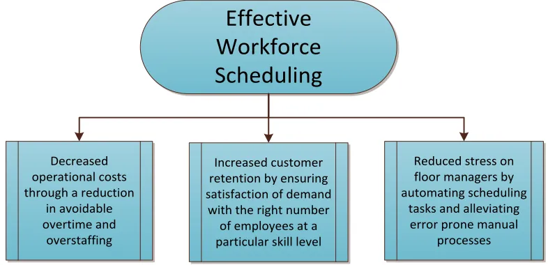
necessitates a highly optimized manufacturing process. As shown in Figure 1.1, the advantages

of optimized worker schedules are decreased expenses, increased customer retention and reduced

pressure on floor managers.

Effective

Workforce

Scheduling

Decreased operational costs through a reduction

in avoidable overtime and

overstaffing

Increased customer retention by ensuring satisfaction of demand

with the right number of employees at a particular skill level

Reduced stress on floor managers by automating scheduling

tasks and alleviating error prone manual

processes

Figure 1.1: Advantages of Effective Workforce Scheduling

For effective scheduling, worker allocation models are popular. As mentioned in Celayix

(2013), the benefits of these models range from lower operating costs, increased customer

into account factors such as allocation of workers with lower qualifications, personal preference

of workers, and pre-allotment of specific workers to specific tasks. Also, parameters such as the

operational cost and the efficiency of workers need to be considered before assignment of the

worker. Sometimes, in labor-intensive tasks, multiple workers are needed for machines and/or

overtime, along with training of workers. Workforce planning, in general, also involves strategic

decisions such as the number of workers which are to be hired, trained or moved to other shifts

for a larger planning horizon.

Worker allocation models must be developed considering different factors, such as type of

work, planning periods, and demand patterns. A few of these factors are given as follows.

• Planning Horizon: We consider three planning horizons; single shift planning, multiple

shift planning and strategic planning. Strategic planning models are generally long-term,

whereas single-shift and multiple-shift planning are short-term.

• Demand Type: The demand can be expressed in a number of ways. For example, it can

be the number of shifts of production needed, the number of workers needed at each

operation, or the number of units produced in one shift.

• Shift Structure: Proper management of the labor force is a daunting task. In particular,

assigning workers to different tasks involving regular work, overtime shifts and training

procedures is a challenge.

• Other Factory Rules: These are rules that are specific to the factory floor under

consideration. Some examples of factory rules are limits on cross-training/overtime per

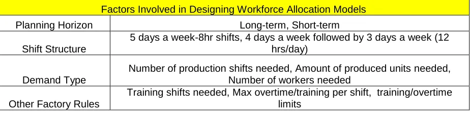
Table 1.1 shows the some examples of planning horizons, shift structure and the demand

type associated with workforce allocation models.

Factors Involved in Designing Workforce Allocation Models

Planning Horizon Long-term, Short-term

Shift Structure

5 days a week-8hr shifts, 4 days a week followed by 3 days a week (12 hrs/day)

Demand Type

Number of production shifts needed, Amount of produced units needed, Number of workers needed

Other Factory Rules

Training shifts needed, Max overtime/training per shift, training/overtime limits

Table 1.1: Factors considered while designing worker allocation models

In a competitive industry, it is imperative to achieve production targets on time, and for

this purpose, workers need to be assigned to operations optimally, such that the demand at every

operation is met. A mismatch between the available workers and the workers needed causes

workforce gaps that result in a loss of profit and goodwill for the manufacturer. Similarly, each

company has its own set of rules that need to be followed throughout the production process.

These rules may be related to machinery, workforce, schedules, and skill qualification. This

work is an industry-motivated project that aims to schedule regular work, overtime work and

cross-training such that workforce gaps are minimized. Also, factory rules are given high

importance, and we observe the effects that these have on individual worker-task allocations.

Skill level considerations also form an important component of the mathematical model, along

with standard factory floor limitations.

The rest of this thesis is organized as follows. Section 2 surveys the literature related to

worker allocation and cross-training models and also highlights the research gap. Section 3

describes the problem and describes the industry-based system under consideration. This section

structure of cost parameters and the implementation architecture. Section 4 contains a numerical

example of the mathematical model developed in Section 3. Section 5 presents the summary of

test cases and experimentation. Also, we discuss the solving time associated with the model and

its overall impact. Section 6 concludes this thesis and proposes future extensions to this research

2. LITERATURE REVIEW

The literature related to this research can be divided into two parts, worker allocation

models, and cross-training models. The discussion of worker allocation models is presented in

Section 2.1 and the discussion of cross-training models is presented in Section 2.2. Section 2.3

highlights the research gap that this work aims to fill.

2.1 Worker Allocation Models

Existing literature in the area of worker allocation can be divided broadly into three areas:

single-shift models, multi-shift models and strategic models. Although we develop a multi-shift

model in this thesis, we have reviewed relevant literature related to single shift models too, since

they are building blocks for multi-shift allocation models. We also present an overview of related

strategic models. Review papers such as Wang (2005) and Ernst et al (2004) perform an

overview of the different personnel scheduling papers. Ernst et al (2004) divides allocation

models according to various parameters such as demand modeling, days off, shift scheduling and

task/shift assignment. Wang (2005) provides an overview of the different application areas such

as healthcare, emergency services, airlines and hotels. A discussion of the individual papers

directly relevant to this research work is provided in the sections below.

2.1.1 Single-Shift Models

Suer (1996) designs an optimal assignment policy for a single period allocation problem

by designing a mixed integer program to determine the operator allotment for a variety of

demand scenarios. The results show that before implementation of this methodology, all

model is applicable for both continuous production and cyclic production. Brusco and Johns

(1998) develop an integer programming model that minimizes the workforce staffing costs for a

single work shift. Different cross-training configurations are evaluated and the model is used to

analyze these configurations. The results indicate that asymmetric training configurations allow

better operator-skill relationships. Campbell (1999) formulates a single shift assignment problem

that considered various skill levels across different departments of an organization. The paper

concludes that the approach used is better than the Lagrangian approach used by other authors.

Askin and Huang (2001) develop two MILP formulations that determine allocation of workers

with different costs for training on different skill levels. The output of the first model assigns

workers to cells and gives the assignment of tasks for the worker at that particular cell. The

second model determines the individual training schedule. Norman et al (2002) considers human

skills such as leadership and decision making while assigning workers. A mixed integer program

is developed to maximize the profit which is expressed in the form of a function of training cost

and throughput. The results indicate that better results occur when only technical skills are

considered. Wu and Fu (2005) present a linear programming model for operator staffing and

assignment in a foundry fab. Their model minimizes the cost of staffing and chooses a staffing

position which is assigned to an operator.

Kuo and Yang (2006) solve an operator allocation problem using mixed integer

programming where the formulation assumes that there is no difference between the skill levels

of operators. It was concluded that this assumption does not hold true when there is significant

difference in between skill levels. Jarugumilli et al (2010) consider rules such as the lower limit

on the number of workers at a machine group, the desired mix of workers with a certain skill

knowing the most effective allocation of resources despite not always being able to meet the

worker requirements. A two-phase goal programming formulation is used which minimizes the

cost of assigning workers and the slack/surplus of workers at each operation. The cost structure

is specified for the parameters used in the optimization. The results indicate that operations and

workers for cross-training can be identified using the model.

2.1.2 Multi-shift Models

In Burns et al (1998), an algorithm for scheduling workforce over 4-day or 3-day work

week is developed. Employees work 4-days a week, have a fixed number of weekends off and

work a maximum of 5 days in a row without a break. The results of the model calculate the

minimum number of workers required to satisfy the demand. Azmat and Widmer (2004),

develop a three-step process for workforce planning and scheduling. First, the minimum

workforce that can satisfy the particular demand is computed. Second, the number of overtime

hours and days off for the workforce is determined. And the last step is the actual allocation of

the number of work days per week to each worker. The results show that the algorithm is a quick

method to allocate workers. Laporte and Pesant (2004) develop a constraint programming

algorithm that can handle a wide variety of constraints during a 24 hour, 7 days a week

manufacturing facility. The algorithm is also validated with computational results which support

their considerations of different shift structures, days off and breaks. Bhatnagar (2007) develops

a linear programming model for optimal allocation of workers for companies such as computer

manufacturers and cellphone makers. The results indicate that the cost of allocation increases

Suer and Tummaluri (2008) expand their single-shift model (Suer, 1996) by considering

a case of multiple periods, operator skill levels and operation times. A heuristic for operator

allotment is developed and considers learning/forgetting issues for a worker. Results show that

the proposed approaches in operator assignment outperform the classical approach of using

standard times. Jaurugmilli (2011) extends his single-shift model (Jarugumilli et al, 2010) by

linking the single-shift and multi-shift decision making scenarios. A multi-shift model is

formulated that makes both single-shift and multi-shift decisions for a two-week planning

horizon. The multi-shift decisions satisfy capacity plans and worker availability constraints,

while the single-shift decisions satisfy qualification and skill level requirements. The results help

workers in identifying operations and workers for cross-training. Also, the model considers

partial allocations for any shift during the planning period.

2.1.3 Strategic Models

Strategic models generally consist of a longer time horizon and often have stochastic

parameters. For instance, Ahn et al (2005) design a Markov decision process that determines the

number of workers to hire while minimizing the cost. Hiring and firing of workers is considered

along with a random demand scenario and linear costs. A dynamic programming based approach

is followed to obtain the optimal staffing levels. Gans and Zhou (2002) also implement a Markov

Decision Processes to determine an optimal policy to determine the number of workers to hire.

The results indicate that the when learning is high, a state dependent policy outperforms a policy

dependent on the number of workers in a system. Huang and Song (2007) use a successive

convex approximation method to model a multi-stage stochastic model. Numerical experiments

Techawiboonwong and Yenradee (2003) consider an aggregate production planning

model using mixed integer programming where the worker resources can be transferred along

production lines. The output provides benefits to managing the available production capacity by

using workforce transfers among the lines. Fowler et al (2007) use MIP to determine different

staffing decisions such as hiring, firing and cross-training to minimize workforce related costs

over multiple periods. Kulkarni et al (2013) uses a scenario-based approach to solve a workforce

planning problem formulated as a two-stage stochastic recourse program. Considerations include

fluctuating demand over a long planning horizon, business and labor rules, e.g., hiring, firing,

overtime, cross-training, and shift swapping. The results indicate that the cost of workforce

formulation can be reduced by using the recourse problem.

2.2 Cross-training Models

Early literature consists of industry implementations of cross-training and its benefits to

individual workers. Hackman and Oldham (1980) talk about the positive effect that

cross-training has on a worker’s quality of life and motivation. Jordan and Graves (1995)provide an

actual guideline for management on the methods used to implement cross-training policies in a

manufacturing environment. In Brandt (1997), an example of a cross-training policy was

CTRAIN, used in semiconductor manufacturing at IBM. The results showed an increase in

teamwork and reduced the pressure felt by workers to adapt to ever-changing demands. Another

work, Bailey (1998), talks about the importance of forming cross-functional teams. This work

also compares different team structures (with a particular level of cross-training) and their

associated with the highest productivity. Slomp and Molleman (2002) distinguish four

cross-training policies depending on their effect on important performance metrics such as load of the

bottleneck workers and the number of new qualifications used. It is shown that a worker oriented

cross-training policy, which spreads functions evenly among employees, performs well.

Hopp and Van Oyen (2003) prove that worker coordination, team structure and training

efficiency are parameters essential in evaluating workforce agility. Also, workforce agility is

supported by cross-training and leads to increased task responsiveness, improved quality of

products, and an increased capability to produce a wider range of products. Slomp et al (2003)

include cross-training into an integer programming formulation that minimizes the cost

associated with training. Also, the model is tested with different values of redundancy of

machines and multi-functionality of workers. The purpose of the formulation is to achieve equal

distribution of workload among the workers. Once the amount of cross-training required has

been determined, a strategy needs is developed to assign workers to training. Bokhorst, et al

(2004) extends on Slomp et al (2003) using the concept of skill chaining to develop different

cross-training configurations.Hopp et al (2004), goes in a different direction from Hopp and Van

Oyen (2003), and analyzes the benefits of cross-training of workers for serial production lines.

Bokhorst (2010) measures the impact of the work-in-process on the use of cross-training skills

received by a worker.

Literature Single-shift /Multi-shift/ Strategic

Overtime Allocations

Cross-training

Multiskilling Considered

Non-stop Production

Fractional Allocation Askin and Huang

(2001) Single-shift √ √ √

Aykin (1996) Single-shift √ √

Azmat and Widmer

(2001) Single-shift √ √

Bokhorst et al (2004) Single-shift √ √

Brusco and Johns

(1998) Single-shift √ √

Campbell (1999) Single-shift √ √

Kuo and Yang (2006) Single-shift √

Norman et al (2002) Single-shift √ √

Slomp and Molleman

(2002) Single-shift √ √

Bhatnagar et al (2007) Multi-shift √ √ √

Fowler et al (2008) Multi-shift √ √

Gomar et al (2002) Multi-shift √

Jarugumilli (2011) Multi-shift √ √ √ √

Subramanian and An

(2008) Multi-shift √ √ √ √

Ahn et al (2005) Strategic √ √

Gans and Zhou (2002) Strategic √

Huang and Song

(2007) Strategic √ √

Techawiboonwong

and Yenradee (2003) Strategic √

Fowler et al (2007) Strategic √ √

Kulkarni et al (2013) Strategic √ √ √ √

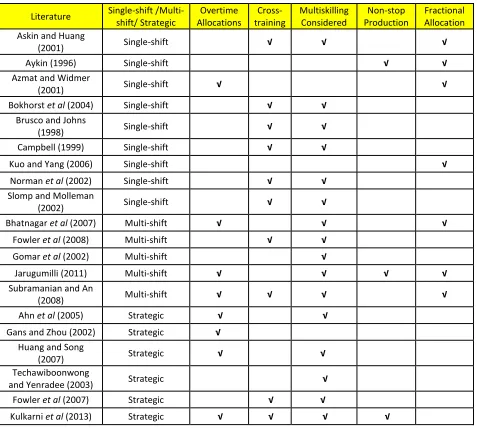
Table 2.2.1: Comparison of selected works of workforce allocation and cross-training

2.3 Research Gap

Figure 2.3.1 describes relevant papers from workforce allocation, cross-training and the

intersection of both. From the papers in the intersection, i.e., Brusco and Johns (1998) and Askin

and Huang (2001), skill levels are relevant, but both are single-shift models. Brusco and Johns

Huang (2001) propose two models developed for only cellular manufacturing systems, and focus

on the synergy between the teams instead of minimizing allocation cost.

As mentioned in Jarugumilli (2011) - to satisfy the different demand scenarios, existing

workforce capabilities might not be sufficient. This results in workforce gaps that result in

unsatisfied demand at the manufacturing floor operations. In previous models such as Bhatnagar

(2007), gaps have been minimized by the use of a large number of overtime workers (i.e.

workers from other shifts) to satisfy the demand of the current shift. However, the use of

overtime workers is a shift-by-shift solution. Over a larger time duration, implementation of

cross-training is needed. Hence, this work integrates cross-training procedures along with regular

and overtime allocation.

As can be observed from Table 2.2.1, we plan to develop a multi-shift model that

integrates regular/ overtime/training allocations, multiskilling, non-stop production and fractional

allocation in the same formulation. In addition, this work also considers many specific factory

3. PROBLEM DESCRIPTION AND FORMULATION

Consider a system that has a fixed number of workers, operations, shifts and skill levels. The

problem involves optimally allocating regular workers, assigning overtime, and assigning

workers for cross-training such that the cost of all three actions along with the cost of the

workforce gaps is minimized.

Depending on the system under consideration, a worker can have a number of skill levels.

Lower skill levels involve doing regular work, and advanced skill levels are related to machine

maintenance. Worker assignments can be made to only one operation at a time at one skill level,

but the worker can be assigned to multiple operations in the same shift.

In case of worker assignment, a worker can work on an operation for some duration of his

shift, while in case of training, a worker has to work for the complete duration of the

cross-training period. If lower skill level cross-training is taking place on an operation, then that operation

can be used by another worker. If higher skill level training is taking place, then that particular

operation cannot be used for any other activity. Every operation has a minimum threshold limit

for which a worker can be assigned to it

There is a set of specified workers for each shift, known as the regular workers. Overtime

workers are regular workers from other shifts who can be contacted if the requirements are not

met by regular workers. Different sets of workers work shifts on fixed days. Based on the

workers working on that particular day, each shift can be classified as part of a shift type.

Workers cannot work in back-to-back shifts, but they can do overtime work in a shift of another

3.1 System under Consideration

The aim is to minimize the costs associated with regular allocation, overtime allocation,

cross-training and workforce gaps. These costs are not monetary costs, but values associated

with the assignment of regular work, overtime, cross-training or gaps. The cost parameters have

been determined based on industry feedback. The structure of these costs will be explained in

Section 3.3.

For the testing and analysis of the model, we have considered a system that includes the

different factors associated with the problem. The components of the system under consideration

are explained below.

3.1.1 Workers/Shifts/Shift Types

This facility has two non-overlapping daily shifts of 12 hours each. There is a fixed

planning horizon of two weeks, i.e., a total of 28 shifts. There are four types of shifts - ST1, ST2,

ST3 and ST4. ST1 and ST3 are daytime shifts, while ST2 and ST4 are night time shifts. Workers

in ST1 and ST2 work for forty-eight hours in week 1 of the planning period, and for thirty-six

hours in week 2 of the planning period. Similarly, workers in ST3 and ST4 work for thirty-six

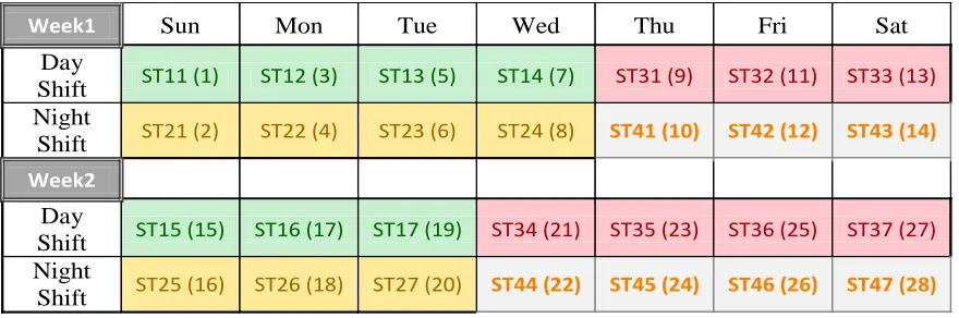
hours in week 1 and forty-eight hours in week 2. Table 3.1.1 shows the shift distribution for the

Table 3.1.1: Shift Structure Considered

To explain the notation, ST13 means that it is shift type 1 (ST1) and the third shift in the

time horizon. So, the general notation is ST[Shift type][Shift number in shift type]. The numbers

in parentheses show the shifts in the order of actual occurrence.

Every shift type contains a set of workers, and apart from overtime situations they work

in shifts of that particular shift type itself. For example, let us say that there are 60 workers; and

workers 1-15 only work in ST1, 16-30 only work in ST2, 31-45 only work in ST3, and 46-60

only work in ST4. These are called as the regular workers for each shift. ST1 and ST2 workers

work day/night shifts on the same day, while ST3 and ST4 workers work day/night shifts on the

same day. Workers in ST3 and ST4 can do overtime work only in shifts ST1 and ST2 (since they

are on different days) and vice versa (i.e., ST1, ST2 workers can do overtime only in ST3 and

ST4).

3.1.2 Skill Levels

A worker can have three skill level qualifications; L1, L2, and L3. L1 is a basic skill

level; L2 and L3 are advanced skill levels that include machine repair and maintenance. Every

operation needs workers that are qualified on L1, L2 and L3. Workers that are qualified on a

Week1 Sun Mon Tue Wed Thu Fri Sat

Day

Shift ST11 (1) ST12 (3) ST13 (5) ST14 (7) ST31 (9) ST32 (11) ST33 (13) Night

Shift ST21 (2) ST22 (4) ST23 (6) ST24 (8) ST41 (10) ST42 (12) ST43 (14)

Week2

Day

Shift ST15 (15) ST16 (17) ST17 (19) ST34 (21) ST35 (23) ST36 (25) ST37 (27) Night

higher skill level (L2 or L3) of a particular operation are capable of doing work at lower skill

levels for the same operation. For example, if a worker is qualified on L3, he can do

OP7-L2 and OP7-L1. If he is qualified on OP7-OP7-L2, he can do OP7-L1 also. However, if he is qualified

on OP7-L1, he cannot do work at OP7-L2 or OP7-L3. Also, to be cross-trained on OP7-L2, a

worker needs to be qualified on OP7-L1; and to be cross-trained on OP7-L3, a worker needs to

be qualified on OP7-L2.

3.1.3 Operations

Every operation has a fixed requirement, i.e., for workers qualified on L1, L2 and L3 on

that operation. Overtime workers (regular workers from other shifts) can be contacted if the

demand for workers is not met by the regular workers on any operation. Every operation is

unique, and a worker that is qualified on an operation skill level combination, cannot

automatically perform work of the same skill level on other operations. Hence, it is essential to

determine the number of workers that need to be qualified on any particular operation. The

solution to the problem involves optimally (at the lowest cost) assigning workers to operations

such that worker requirement at every skill level, on every operation is met. If regular workers

are not sufficient then overtime workers from other shifts (not shifts on the same day) are used.

The two-week schedule for normal allocation of workers and that for cross-training of workers

needs to be developed before the start of each planning period.

Figure 3.1.1 denotes the normal operating procedure of the factory floor. The initial

scenario depicts workers slotted into the 4 different shift types, i.e., workers 1-4 in ST1, workers

5-7 in ST2, and so on. The same operations exist for each shift of a shift type, and each operation

allocation of workers, cross-training of workers, and overtime allocations (if needed) from other

shift types take place. For example, for ST1, overtime on an operation is obtained from workers

in ST3 and/or ST4. ST2 cannot provide overtime workers because it would mean that a worker,

if assigned for overtime in this shift, would work for 24 hours non-stop. Similarly, for ST2

overtime is obtained from ST3 and/or ST4 and for ST3 and ST4, overtime is obtained from ST1

and/or ST2. If even after assigning overtime, the demand is not satisfied, then workforce gaps are

created.

ST3

W08,W09,W10,W11

Regular Allocations Cross-training

ST1

W01,W02,W03,W04

Regular Allocations Cross-training

ST2

W05,W06,W07

Regular Allocations Cross-training

ST4

W12,W13,W14,W15

Regular Allocations Cross-training

O

ve

rt

im

e

Overti_me

Overt ime

O

ve

rt

im

e

3.2 MULTI-SHIFT CROSS-TRAINING MODEL

To integrate regular, overtime and cross-training assignments, we develop a multi-shift

cross-training model formulated as an MIP model. It is a deterministic formulation for a fixed

time horizon and the assignment of workers and cross-training schedules are developed for each

shift. The regular work requirements and the cross-training requirements are known entities, and

the aim is to satisfy these values while minimizing the cost associated with regular allocations,

overtime allocations, cross-training assignments and workforce gaps and cross-training gaps.

Other factory floor considerations have also been taken into account in the formulation.

3.2.1 Notation

The notation used in the mathematical model is given as follows:

Sets

𝑠𝑒𝑡 𝐼 = {1,2, … . . I} is the set of workers.

𝑠𝑒𝑡 𝑁 = {1,2, … . N} is the set of operations.

𝑠𝑒𝑡 𝐿 = {1,2, … . . L} is the set of skill levels.

𝑠𝑒𝑡 𝐾 = {1,2, … . K} is the set of shifts.

𝑠𝑒𝑡 𝐽 = {1,2, . . J} is the set of shift types.

𝑠𝑒𝑡 𝐾𝑗 = Set of shifts present in shift type 𝑗 𝜖 𝐽.

Variables

𝑆_𝑖𝑙𝑛𝑗𝑘 = Binary variable which is 1 if training starts for worker 𝑖 𝜖 𝑊_𝑗, on skill level 𝑙 𝜖 𝐿, operation

𝑛 𝜖 𝑁, during shift type 𝑗 𝜖 𝐽 and shift number 𝑘 𝜖 𝐾_𝑗, and 0 otherwise.

𝑋_𝑖𝑙𝑛𝑗𝑘 = Continuous variable from 0 to 1 which denotes the percentage of the shift duration for

worker 𝑖 𝜖 𝑊_𝑗, on skill level 𝑙 𝜖 𝐿, operation 𝑛 𝜖 𝑁, during shift type 𝑗 𝜖 𝐽 and shift number 𝑘 𝜖 𝑇_𝑗.

𝑌_𝑖𝑙𝑛𝑗𝑘 = Binary variable which is 1 if worker 𝑖 𝜖 𝑊_𝑗 is being trained on skill level 𝑙 𝜖 𝐿, operation

𝑛 𝜖 𝑁, during shift type 𝑗 𝜖 𝐽 and shift number 𝑘 𝜖 𝑇_𝑗, and 0 otherwise.

𝑂𝑇_𝑙𝑛𝑗𝑘 = Amount of overtime worker-shifts needed for operation 𝑛 𝜖 𝑁, skill level 𝑙 𝜖 𝐿 during

shift type 𝑗 𝜖 𝐽 and shift number 𝑘 𝜖 𝐾_𝑗.

𝐺_𝑙𝑛𝑗𝑘 = Gap in the allocation at operation 𝑛 𝜖 𝑁, on skill level 𝑙 𝜖 𝐿 during shift type 𝑗 𝜖 𝐽 and shift

number 𝑘 𝜖 𝐾𝑗.

𝐸_𝑖𝑙𝑛𝑗𝑘 = Binary variable which is 1 when worker 𝑖 𝜖 𝑊𝑗 on operation 𝑛 𝜖 𝑁 and skill level 𝑙 𝜖 𝐿 is

being trained during shift type 𝑗 𝜖 𝐽 and shift number 𝑘 𝜖 𝐾𝑗, and the training ends in shift k-1,

and 0 otherwise.

𝑆𝐿_𝑙𝑛, 𝑆𝑃_𝑙𝑛 = Slack variable and surplus variable which denote the gap in cross-training on

operation 𝑛 𝜖 𝑁 and skill level 𝑙 𝜖 𝐿.

𝑍_𝑖𝑙𝑛𝑗𝑘 = Binary variable that is 1 if worker 𝑖 𝜖 𝑊𝑗 is assigned to operation 𝑛 𝜖 𝑁, skill level 𝑙 𝜖 𝐿

𝑇𝑊_𝑛𝑗𝑘 = Binary variable that is 1 if training of skill level L2 or L3 is taking place at n 𝜖 𝑁 in shift

type 𝑗 𝜖 𝐽, shift 𝑘 𝜖 𝐾𝑗. It is 0 otherwise.

𝑆𝑇_𝑙𝑛𝑗𝑘 = Binary variable that is 1 if training takes place on operation n, skill level l in shift type

𝑗 𝜖 𝐽, and shift 𝑘 𝜖 𝐾_𝑗, and 0 otherwise.

Parameters

𝑟_𝑙𝑛𝑗 = Number of worker-shifts needed on operation 𝑛 𝜖 𝑁 and skill level 𝑙 𝜖 𝐿 during shift type

𝑗 𝜖 𝐽.

𝑟𝑐𝑙𝑛 = Number of worker-shifts of training needed on operation 𝑛 𝜖 𝑁 and skill level 𝑙 𝜖 𝐿.

𝑚𝑠ℎ𝑖𝑓𝑡𝑙𝑛 = Number of shifts of training needed for a worker to be completely trained on

operation 𝑛 𝜖 𝑁 and skill level 𝑙 𝜖 𝐿.

𝑚𝑛/𝑚𝑥 = Minimum/maximum number of qualifications a worker can have at any moment in

the time horizon.

𝑐_𝑖𝑙𝑛 = Cost of assignment for worker 𝑖 𝜖 𝐼, on skill level 𝑙 𝜖 𝐿 and operation 𝑛 𝜖 𝑁.

𝑐𝑡_𝑖𝑙𝑛 = Cost of training worker 𝑖 𝜖 𝐼, on skill level 𝑙 𝜖 𝐿 and operation 𝑛 𝜖 𝑁.

𝜖_𝑖𝑙𝑛𝑗𝑘 = Pre-allocation if training has been carried forward for worker 𝑖 𝜖 𝑊_𝑗, on skill level 𝑙 𝜖 𝐿

𝜑_𝑖𝑙𝑛𝑗𝑘 = Partial allocation for cross-training that is given to the worker 𝑖 𝜖 𝑊𝑗, on skill level 𝑙 𝜖 𝐿

and operation 𝑛 𝜖 𝑁, in shift type 𝑗 𝜖 𝐽 and shift number 𝑘 𝜖 𝐾𝑗.

𝑞𝑖𝑙𝑛 = Value is 1 if worker 𝑖 𝜖 𝑊𝑗, is qualified at skill level 𝑙 𝜖 𝐿 and operation 𝑛 𝜖 𝑁 at the

beginning of the planning period, and 0 otherwise.

𝑜𝑡_{𝑙𝑖𝑚𝑖𝑡} = Limit on overtime for the entire factory.

∝𝑠ℎ𝑖𝑓𝑡 = Limit on training for every shift.

𝛽_{𝑓𝑎𝑐𝑡𝑜𝑟𝑦} = Limit for training for the complete factory.

𝑝𝑙𝑛 = Cost of overtime on operation 𝑛 𝜖 𝑁 and skill level 𝑙 𝜖 𝐿.

𝑝𝑠𝑙𝑛= Cost of a gap at operation 𝑛 𝜖 𝑁 on skill level 𝑙 𝜖 𝐿.

𝑝𝑝_𝑙𝑛, 𝑝𝑛_𝑙𝑛 = Cost of surplus/slack in cross-training on operation 𝑛 𝜖 𝑁 and skill level 𝑙 𝜖 𝐿.

𝑀 = A big number (condition : 𝑀 ≥ 1/𝑠𝑚)

𝑠𝑚 = Lowest allocation that a worker can take if he is assigned (Eg: If assigned, the worker can

take a value of greater than 0.1).

𝑐𝑜𝑢𝑛𝑡_𝑖 = Number of individual operation-skill level qualifications a worker 𝑖 𝜖 𝑊_𝑗 possesses at

the beginning of the shift.

𝑡𝑙 = Upper limit on the number of worker than can be trained on an operation in any particular

shift.

𝐿𝑖𝑚 = Number of times a worker can be trained over the planning horizon.

3.2.2 Mathematical Model

The data in the previous section is used to formulate the mathematical model that can be given as

follows.

Objective Function

The objective function [1] is a cost-parameter based formula that minimizes the sum of the

following:

 Total cost of assignment of regular workers on all the operations over two weeks,

 Total cost of all overtime assignments over the two weeks,

 Penalty costs due to all the operations where workforce gaps exist over two weeks,

 Total cost of cross-training workers over two weeks, and

 Penalty costs associated with not meeting cross-training targets that are specified at the

beginning of the two weeks.

Minimize ∑ ∑ ∑ ∑ ∑ 𝑐_{𝑙 𝑖 𝑛 𝑘 𝑗 𝑖𝑙𝑛}. 𝑋_𝑖𝑙𝑛𝑗𝑘 + ∑ ∑ ∑ ∑ 𝑝_{𝑙 𝑛 𝑘 𝑗 𝑙𝑛} . 𝑂𝑇_𝑙𝑛𝑗𝑘+ ∑ ∑ ∑ ∑ 𝑝𝑠_{𝑙 𝑛 𝑘 𝑗 𝑙𝑛}. 𝐺_𝑙𝑛𝑗𝑘+

∑ ∑ ∑ ∑ ∑ 𝑐𝑡𝑖𝑙𝑛. 𝑌𝑖𝑙𝑛

𝑗𝑘 𝑗

𝑘 𝑛 𝑙

Constraints

Constraint [2] ensures that the total worker allocation at each operation (including overtime

allocations) should satisfy the requirement at that operation in each shift. If it does not, then

worker gaps are observed. Similarly, even the cross-training requirements are given. Constraint

[3] ensures that the number of workers trained on every operation over the two weeks should be

equal to the pre-established targets.

∑ 𝑋_{𝑖 𝑖𝑙𝑛}𝑗𝑘 + 𝑂𝑇_𝑙𝑘𝑗𝑘+ 𝐺_𝑙𝑛𝑗𝑘 = 𝑟_𝑙𝑛𝑗 ∀ 𝑙, 𝑛, 𝑗, 𝑘 [2]

∑ ∑ ∑ 𝑌𝑖 𝑗 𝑘 _𝑖𝑙𝑛𝑗𝑘− 𝑆𝑃𝑙𝑛+ 𝑆𝑁𝑙𝑛 = 𝑟𝑐𝑙𝑛 ∀ 𝑙, 𝑛 [3]

Constraints [4] and [5] work together. If a worker is allocated, he can only be allocated for a shift

duration that is greater than or equal the minimum limit, sm. Generally, for most test cases, we

have assumed this value to be 25% of the total shift duration.

𝑍_𝑖𝑙𝑛𝑗𝑘 ≥ 𝑋_𝑖𝑙𝑛𝑗𝑘 ∀ 𝑖, 𝑙, 𝑛, 𝑗, 𝑘 [4]

𝑍_𝑖𝑙𝑛𝑗𝑘 ≤ 1

𝑠𝑚. 𝑋𝑖𝑙𝑛 𝑗𝑘

∀ 𝑖, 𝑙, 𝑛, 𝑗, 𝑘 [5]

Constraint [6] ensures that the total overtime allocation for the factory does not cross an upper

limit. Constraint [7] ensures that a worker cannot be assigned to training while doing work, and

vice versa. There are upper limits on the number of workers cross-trained per shift as given in

Constraint [8], and the number of workers that can be cross-trained in the planning period as

∑ ∑ ∑ ∑𝑙 𝑛 𝑗 𝑘𝜖𝐾𝑗𝑂𝑇_𝑙𝑛𝑗𝑘 ≤ 𝑜𝑡_𝑙𝑖𝑚𝑖𝑡 [6]

∑ ∑ 𝑋_{𝑙 𝑛 𝑖𝑙𝑛}𝑗𝑘 + ∑ ∑ 𝑌_{𝑙 𝑛 𝑖𝑙𝑛}𝑗𝑘 ≤ 1 ∀ 𝑖 𝜖 𝑊_𝑗, 𝑗 𝜖 𝐽, 𝑘 𝜖 𝐾_𝑗 [7]

∑ ∑ ∑ 𝑌_{𝑖 𝑙 𝑛 𝑖𝑙𝑛}𝑗𝑘 ≤ ∝_{𝑠ℎ𝑖𝑓𝑡} ∀ 𝑗 𝜖 𝐽, 𝑘 𝜖 𝐾_𝑗 [8]

∑ ∑ ∑ ∑ ∑ 𝑌𝑙 𝑛 𝑘 𝑗 𝑖 _𝑖𝑙𝑛𝑗𝑘≤ 𝛽𝑓𝑎𝑐𝑡𝑜𝑟𝑦 [9]

Constraints [10] and [11] address the fact that if a worker starts, then the starting shift needs to

be kept track of)

𝑆_𝑖𝑙𝑛𝑗𝑘 = 𝑌_𝑖𝑙𝑛𝑗𝑘 ∀ 𝑖 𝜖 𝑊𝑗, 𝑙 𝜖 𝐿, 𝑛 𝜖 𝑁, 𝑗 𝜖 𝐽, 𝑘 = 𝑘𝑗[1] 𝜖 𝐾𝑗 [10]

𝑆_𝑖𝑙𝑛𝑗𝑘 ≥ 𝑌_𝑖𝑙𝑛𝑗𝑘− 𝑌_𝑖𝑙𝑛𝑗𝑘′ ∀ 𝑖, 𝑙, 𝑛, 𝑗, 𝑘 > 𝑘_𝑗[1] , 𝑘′_{= 𝐸𝑙𝑒𝑚𝑒𝑛𝑡 𝑜𝑓 𝐾}

𝑗 𝑏𝑒𝑓𝑜𝑟𝑒 𝑘 𝜖 𝐾𝑗 [11]

Constraint [12] satisfies the requirement that if a worker is has started training, then he must be

trained for the pre-specified number of shifts needed to be qualified at that skill level.

𝑚𝑠ℎ𝑖𝑓𝑡_𝑙𝑛. 𝑆_𝑖𝑙𝑛𝑗𝑘 ≤ ∑𝑟 ≤𝑘′=𝑘+𝑚𝑠ℎ𝑖𝑓𝑡𝑙𝑛−1𝑌_𝑖𝑙𝑛𝑗𝑟

𝑟 ≥ 𝑘 ∀ 𝑖 𝜖 𝑊𝑗, 𝑙, 𝑛, 𝑗, 𝑘 𝜖 𝐾𝑗, 𝑘 ′_{𝜖 𝑇}

𝑗 [12]

Constraint [13] prevents duplicate training of a particular worker on the same operation-skill

level combination.

∑_{𝑘 𝜖 𝐾} 𝑆_𝑖𝑙𝑛𝑗𝑘

The shift in which training for a worker ends is kept track of using Constraints [14] and [15].

Constraint [14] recognizes the ending shift, and if training shifts are more than 1, Constraint [15]

ensures that the variable denoting the end of training is 0 in the shifts between the start and end

shifts.

𝑆_𝑖𝑙𝑛𝑗𝑘 = 𝐸_𝑖𝑙𝑛𝑗𝑘′ ∀ 𝑖, 𝑙, 𝑛, 𝑗, 𝑘 𝜖 𝐾𝑗 , 𝑘′= (𝑚𝑠ℎ𝑖𝑓𝑡𝑙𝑛+ 𝑘)𝑡ℎ 𝑚𝑒𝑚𝑏𝑒𝑟 𝑜𝑓 𝑇𝑗 [14]

Only if 𝑚𝑠ℎ𝑖𝑓𝑡𝑙𝑛> 1;

𝐸_𝑖𝑙𝑛𝑗𝑘 = 0 ∀ 𝑖, 𝑙, 𝑛, 𝑗, 𝑘 ≤ (𝑚𝑠ℎ𝑖𝑓𝑡𝑙𝑛)𝑡ℎ 𝑚𝑒𝑚𝑏𝑒𝑟 𝑜𝑓 𝑇𝑗 && 𝑘 𝜖 𝐾𝑗 [15]

Constraints [16] and [17] put lower and upper limits on the number of possible qualifications a

worker can have in any shift.

∑ ∑ ∑ 𝑆𝑛 𝑙 𝑘 _𝑖𝑙𝑛𝑗𝑘 + 𝑐𝑜𝑢𝑛𝑡𝑖 ≥ 𝑚𝑛 ∀ 𝑖, 𝑗 [16]

∑ ∑ ∑ 𝑆_{𝑛 𝑙 𝑘 𝑖𝑙𝑛}𝑗𝑘 + 𝑐𝑜𝑢𝑛𝑡_𝑖 ≤ 𝑚𝑥 ∀ 𝑖, 𝑗 [17]

Constraint [18] enforces that a worker can only be trained on skill level L2 of an operation if he

is qualified on skill level L1 of that same operation. Similarly, Constraint [19] enforces that

condition for L3 and L2.

𝑀. 𝐸_𝑖𝑙𝑛𝑗𝑘 ≥ ∑ 𝑌_𝑖𝑙𝑗𝑘′_𝑛

′

𝑀. 𝐸_𝑖𝑙𝑛𝑗𝑘 ≥ ∑ 𝑌_𝑖𝑙𝑗𝑘′_𝑛 ′

𝑘′_>𝑘 ∀ 𝑙 = 𝐿2, ; 𝑙′ = 𝐿3; 𝑛, 𝑖, 𝑗 && 𝑞_𝑖𝑙𝑛𝑗𝑘 = 0 ∀ 𝑙 = 𝐿2, 𝐿3 [19]

Constraint [20] puts an upper limit on the number of workers that can be trained on the same

operation-skill level combination in the same shift.

∑ ∑ 𝑌_{𝑙 𝑖 𝑖𝑙𝑛}𝑗𝑘 ≤ 𝑡𝑙 ∀ 𝑗 𝜖 𝐽, 𝑘 𝜖 𝑇_𝑗, 𝑛 𝜖 𝑁 [20]

Constraint [21] puts an upper limit on the number of assignments of a worker that can be made in

one shift.

∑ ∑ 𝑍_{𝑙 𝑛 𝑖𝑙𝑛}𝑗𝑘 ≤ 𝑤𝑙 ∀ 𝑗 𝜖 𝐽, 𝑘 𝜖 𝐾_𝑗, 𝑖 𝜖 𝑊_𝑗 [21]

Constraint [22] puts an upper limit on the number of times a worker can be trained during the

planning horizon.

∑ ∑ ∑ 𝑆𝑘 𝑛 𝑙 _𝑖𝑙𝑛𝑗𝑘 ≤ 𝐿𝑖𝑚 ∀ 𝑖 𝜖 𝑊𝑗, 𝑗 [22]

Constraints [23] and [24] ensure that training of skill levels L2 and L3 only occurs if there is no

work currently taking place at the particular operation in that shift.

∑ ∑𝑖 𝑙=𝐿2,𝐿3𝑌_𝑖𝑙𝑛𝑗𝑘 ≤ 𝑀. 𝑇𝑊_𝑛𝑗𝑘 ∀ 𝑗 𝜖 𝐽, 𝑘 𝜖 𝐾𝑗, 𝑛 𝜖 𝑁 [23]

Constraints [25] and [26] enforce the condition that for any operation, in any shift of the

planning horizon, training cannot occur at multiple skills levels.

∑ 𝑌_{𝑖 𝑖𝑙𝑛}𝑗𝑘 ≤ 𝑀. 𝑆𝑇_𝑙𝑛𝑗𝑘 ∀ 𝑙, 𝑛, 𝑗, 𝑘 𝜖 𝑇_𝑗 [25]

∑ 𝑆𝑇𝑙 _𝑙𝑛𝑗𝑘≤ 1 ∀ 𝑗, 𝑛, 𝑘 𝜖 𝑇𝑗 [26]

If there are any pre-allocations for cross-training before the beginning of the planning horizon,

then they can be assigned in the model using Constraint [27].

𝜖_𝑖𝑙𝑛𝑗𝑘 ≤ 𝑌_𝑖𝑙𝑛𝑗𝑘 ∀ 𝑖, 𝑙, 𝑛, 𝑗, 𝑘 [27]

Similarly, the partial allocations assigned in the model before the planning period starts can be

assigned using Constraint [28].

𝜑_𝑖𝑙𝑛𝑗𝑘 ≤ 𝑋_𝑖𝑙𝑛𝑗𝑘 ∀ 𝑖, 𝑙, 𝑛, 𝑗, 𝑘 [28]

Constraint [29] ensures that the duration a worker can be assigned on any operation skill-level

combination in any shift is between 0 and 1, i.e, from 0% of the worker’s shift to 100% of the

worker’s shift.

Constraint [30] specifies the binary variables used in the model.

𝑆_𝑖𝑙𝑛𝑗𝑘, 𝑍_𝑖𝑙𝑛𝑗𝑘, 𝐸_𝑖𝑙𝑛𝑗𝑘, 𝑌_𝑖𝑙𝑛𝑗𝑘, 𝑇𝑊_𝑛𝑗𝑘, 𝑆𝑇_𝑙𝑛𝑗𝑘 𝜖 {0,1} ∀ 𝑖, 𝑙, 𝑛, 𝑗, 𝑘 [30]

3.3 COST PARAMETER STRUCTURE

Here, we present the structure of the cost parameters used in the objective function

presented in the previous sub-section. For every operation skill-level scenario, we can split the

set of workers I in any shift type j, into two groups; 𝐼_𝑙𝑛 – the set of workers qualified on skill

level l and operation n and 𝐼_{𝑙′𝑛′}- the set of workers not qualified on skill level l and operation n.

Also, if worker 𝐼_𝑙𝑛 is present in shift type j, then we denote the worker as 𝐼_𝑙𝑛𝑗 , and if the worker is

not present in shift type j, then we denote the worker as 𝐼_𝑙𝑛𝑗′.

Definition 1: An operation-skill level combination is defined as a particular instance of the

operation and the skill level. For example, if there are three operations - OP1, OP2 and OP3, and

two skill levels – L1 and L2, then the set of operation-skill level combinations is {OP1-L1,

OP2-L1, OP3-OP2-L1, OP1-L2, OP2-L2, OP3-L2}.

Definition 2: A skill level relaxation occurs when there exists a requirement on an operation of a

specific skill level and it is filled by a worker qualified on the same operation but of a lower skill

level.

Theorem 1: This theorem is derived from a theorem in Jarugumilli (2011). If an optimal

solution is to be obtained, the cost of assigning a worker that is qualified on a particular skill

Proof: We need the qualified workers to perform the task, not the ones that are not qualified.

Since, the optimal value of the objective function is a minimization of the costs, we obtain

𝑐𝑖𝑙𝑛 < 𝑐𝑖′𝑙𝑛, 𝑖’ is the worker that is not qualified on skill l and operation n.

Theorem 2: If the cost of allocating any worker qualified on a particular operation-skill level

combination is less than the cost of cross-training any worker on the same operation-skill level

combination, i.e.,𝑐𝑖𝑙𝑛 < 𝑐𝑡𝑥𝑙𝑛, for x = i and x≠i., then we obtain an optimal solution.

Proof:This can be divided into 2 conditions, (𝑖)𝑖 = 𝑥 = 𝐼_𝑙𝑛 𝑎𝑛𝑑 (𝑖𝑖)𝑖 = 𝐼_𝑙𝑛 , 𝑥 = 𝐼_{𝑙′𝑛′}. Also, we

can say that the objective function value for each case is W1 and W2.

For (i), we compare the costs of cross-training and allocation for the same worker. Assuming he

is qualified on OP2-L1, we do not need to assign him to cross-training for OP2-L1. Hence, if

𝑐_𝑖𝑙𝑛 > 𝑐𝑡_𝑥𝑙𝑛, the value W1 would favor cross-training and not allocation. Hence, 𝑐_𝑖𝑙𝑛 < 𝑐𝑡_𝑥𝑙𝑛.

For (ii), we consider a worker that is not qualified on the operation-skill level combination to

another worker that is qualified on it. From Theorem 1, for worker i we obtain 𝑐𝑖𝑙𝑛 < 𝑐𝑥𝑙𝑛.

Also, from part (i) of this theorem, we obtain that 𝑐_𝑥𝑙𝑛 < 𝑐𝑡_𝑥𝑙𝑛. Hence, we can prove that

𝑐_𝑖𝑙𝑛 < 𝑐𝑡_𝑥𝑙𝑛.

Theorem 3: If a skill level relaxation takes place, the cost of assigning a worker to the different

skill level on the same operation is always higher.

Proof: If a skill level relaxation takes place for skill level 𝑙, it means that instead of assigning

worker 𝐼𝑙𝑛 on operation n, we have assigned worker 𝐼𝑙′𝑛 on operation n. This means that one less

worker is available to be assigned on skill level 𝑙’. There is an extra overhead cost that needs to

Theorems 1, 2 and 3 were concerned with comparing the costs for single workers. Now,

we will consider costs for overtime allocation, workforce gap, and slack/surplus in cross-training

for the complete set of workers present in each shift type.

Definition 3: The workforce gap is defined the gap observed at every operation-skill level

combination in each shift in the planning horizon.

Definition 4: The slack and surplus in cross-training is the number of shifts lesser than and

greater than the cross-training targets (specified at the beginning of the planning horizon)

respectively for every operation skill level combination.

Theorem 4: The cost of cross-training surplus is less than the cost of cross-training slack, which

is in turn less than the cost of total overtime per shift which is in turn less than the cost of the

workforce gap per shift.

Proof: We will prove this theorem in parts. (i) 𝑝_𝑙𝑛 < 𝑝𝑠_𝑙𝑛 (ii) 𝑝𝑝_𝑙𝑛 < 𝑝𝑛_𝑙𝑛 (iii) 𝑝𝑛_𝑙𝑛 < 𝑝_𝑙𝑛

The cost of a workforce gap at a particular operation skill level combination is the highest. This

is because a workforce gap causes a shortage in production, and a shortage causes a loss of profit

and reputation for the company. Hence, 𝑝_𝑙𝑛 < 𝑝𝑠_𝑙𝑛 and (i) holds true.

Similarly, a surplus in cross-training targets is preferable as compared to a slack. Hence, 𝑝𝑝_𝑙𝑛 <

𝑝𝑛𝑙𝑛, and (ii) holds true.

We can prove (iii) by negation. The cost parameters need to be structured such that satisfying the

operational demand is a higher priority as compared to worker training. If we assume 𝑝𝑛_𝑙𝑛 >

overtime to meet the extra demand, training assignments will be given a priority in the objective

function. Hence, 𝑝𝑛_𝑙𝑛 < 𝑝_𝑙𝑛.

Tables 3.3.1 and 3.3.2 show an example that denotes the values taken for the cost

parameters in the model. As we can observe from Table 3.3.1, the cost parameters for a worker

qualified at a skill level and performing work at that skill level are the lowest values in the table.

L1 at L1 is 270/271/272, L2 at L2 is 210/211/212 and L3 at L3 is 100/101/102. These three

parameters are in descending order, because L3 work is generally considered more important and

the workers qualified on L3 should be working at L3 instead of working on lower skill levels. It

is to be noted that the specific values themselves are not important as the relationship between

these values.

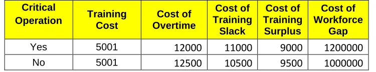
Table 3.3.2 highlights the difference in costs for critical operations. The cost parameters

are close to each other, but the cost of workforce gaps is higher for critical operations, the cost of

training slack is higher and the cost of training surplus is lower for critical operations.

Trained_Skill Level

Performs Work of

Preference 1

Preference 2

Preference 3

L1 L1 270 271 272

L1 L2 5900 5910 5920

L1 L3 6700 6710 6720

L2 L1 2300 2310 2320

L2 L2 210 211 212

L2 L3 5300 5310 5320

L3 L1 1900 1910 1920

L3 L2 1700 1710 1720

L3 L3 100 101 102

Critical

Operation Training Cost

Cost of Overtime

Cost of Training

Slack

Cost of Training

Surplus

Cost of Workforce

Gap

Yes 5001 12000 11000 9000 1200000

No 5001 _{12500 10500 9500 1000000}

Table 3.3.2: Other Cost Parameters

3.4 Implementation Architecture

Figure 3.4.1 shows the implementation architecture for the mathematical model. The input

requirements are converted into a Derived Requirements document, which is then used by a C#

code. The solver used to perform the optimization is IBM ILOG CPLEX 12.4.

Output from Multi-shift Cross-training Model Input to Multi-Shift Cross-training Model

Worker Qualification

Data Operational Requirement and Training

Data

Worker Cross-training List Shift-by-shift Worker Assignment

C# Interface

IBM CPLEX

12.4 Worker

Overtime Allocations Input Format

Requirements

Derived Requirements

Figure 3.4.1: Implementation Architecture

The input requirements are given in terms of values such as man-machine ratio, L1:L2:L3

ratio, and the tool count needed for each shift. These values are then converted in a derived

each operation-skill level combination (additional information on this procedure is given in

Section 4). Similarly, even the training data is specified in the form of number of shifts.

Furthermore, the workers qualification matrix at the beginning of the planning period is also

needed as an input. An example of the input format is shown in the Table 3.4.1, and the

corresponding derived requirements are shown in Tables 3.4.2(a), (b) and (c). The columns of

Table 3.4.1 are described below.

Operation: It is the actual operation under consideration on the manufacturing floor.

MMR (Man-Machine Ratio): The value that is used to convert the amount of workers needed

with respect to the amount actually needed at the machines.

L1:L2:L3: This is the ratio of the requirement for each skill level at every operation.

Tool Count: This denotes the actual machine requirement at each shift type. Hence, here we have

values for ST1, ST2, ST3 and ST4 in each column.

The calculation for each cell in Table 3.4.3 is given as:

L1 Req. = (Tool Count)*MMR*L1 / (L1+L2+L3)

L2 Req. = (Tool Count)*MMR*L2 / (L1+L2+L3)

L3 Req. = (Tool Count)*MMR*L3 / (L1+L2+L3)

The values denote the total number of worker-shifts that are needed to satisfy the requirement for

Table 3.4.1: Input Format

L1 Req. _{ST1 ST2 ST3 ST4}

OP1 0.1 0.1 0.14 0.1 OP2 0.45 0.15 0.25 0.3 OP3 0.2 0.32 0.16 0.28

Table 3.4.2(a): Derived Requirements (L1)

L2 Req. _{ST1 ST2 ST3 ST4}

OP1 0.1 0.1 0.14 0.1 OP2 0.45 0.15 0.25 0.3 OP3 0.2 0.32 0.16 0.28

Table 3.4.2(b): Derived Requirements (L2)

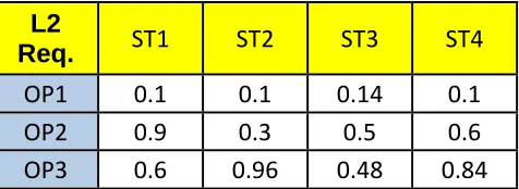
L2

Req. ST1 ST2 ST3 ST4

OP1 0.1 0.1 0.14 0.1 OP2 0.9 0.3 0.5 0.6 OP3 0.6 0.96 0.48 0.84

Table 3.4.2(c): Derived Requirements (L3)

The output of the model provides the shift-by-shift worker assignment, the worker

cross-training list and the worker overtime allocations. The output tables for a numerical example are

Operation MMR L1:L2:L3 Tool Count ST1

Tool Count ST2

Tool Count ST3

Tool Count ST4

Op1 2:3 1:1:1 0.45 0.45 0.63 0.45

Op2 1:2 1:1:2 3.6 1.2 2 2.4

described in detail in Section 4. Section 4 also contains a shift type based view of these

allocations and also an individual shift based view of each worker during the shift.

4. NUMERICAL EXAMPLE

In this section, we discuss a numerical example that has been solved using the integrated

multi-shift cross-training model formulated in Section 3. The specifications of this test case are given

in Table 4.1.

Shifts 28

Shift Types 4

Number of shifts in each Shift Type 7

Workers 15

Operations 5

Skill levels L1, L2, L3

Regulars Worker / Shift type

1-6 (ST1) 7 (ST2) 8-11 (ST3) 12-15 (ST4) Table 4.1: Test Case Specifications

The tables that act as input to the model and output to the model are discussed below.

Tables 4.2 (a), (b) and (c) show the number of shifts of regular allocation (parameter 𝑟_𝑙𝑛 needed

for each operation skill level combination in a shift of each shift type, i.e, these are the derived

L1 Req. ST1 ST2 ST3 ST4

OP1 0.50 1.19 0.51 0.96 OP2 0.51 0.48 0.72 0.50 OP3 0.47 0.42 0.72 0.39 OP4 0.30 0.47 0.60 0.65 OP5 0.33 0.43 0.45 0.49

Total 2.11 3.00 3.00 3.00

Table 4.2(a): L1 Requirements for Test Case

L2 Req. ST1 ST2 ST3 ST4

OP1 0.25 0.25 0.25 0.25 OP2 0.33 0.26 0.25 0.25 OP3 0.27 0.25 0.25 0.25 OP4 0.31 0.25 0.40 0.38 OP5 0.25 0.33 0.34 0.25

Total 1.40 1.34 1.49 1.38

Table 4.2(b): L2 Requirements for Test Case

L3 Req. _{ST1 ST2 ST3 ST4}

OP1 0.28 0.25 0.25 0.25 OP2 0.25 0.31 0.25 0.25 OP3 0.31 0.25 0.25 0.25 OP4 0.25 0.25 0.28 0.25 OP5 0.25 0.33 0.26 0.42

Total 1.35 1.39 1.28 1.42

Table 4.3 denotes the critical operations present on the manufacturing floor. The critical

operations are important to obtain effective production in the manufacturing process. Hence, a

gap at these operations provides more of a problem than a gap faced at other operations.

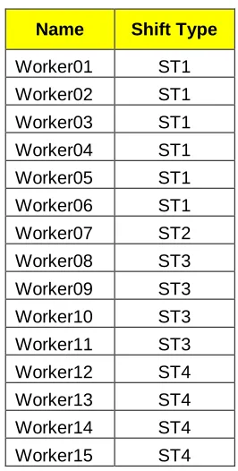
Table 4.4 denotes the workers assigned to each shift type.

Operation Critical Operation

Cross Training Area

Op1 No Assembly

Op2 No Assembly

Op3 Yes Assembly

Op4 No Assembly

Op5 No Assembly

Table 4.3: Critical Operations

Name Shift Type

Worker01 ST1

Worker02 ST1

Worker03 ST1

Worker04 ST1

Worker05 ST1

Worker06 ST1

Worker07 ST2

Worker08 ST3

Worker09 ST3

Worker10 ST3

Worker11 ST3

Worker12 ST4

Worker13 ST4

Worker14 ST4

Worker15 ST4

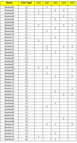
Table 4.5 shows the qualifications of each worker on each operation-skill level combination. The

numbers 1, 2 and 3 denote the preference of the worker on that particular operation. Preference 1

means that the worker prefers to work on this operation as compared to any other operation for

that particular skill level. (Similarly for preference 2 means the worker prefers to work on one

operation before this operation). The fields that do not have any number present indicate that the

worker is not qualified on any of these operations. The workers are eligible to be trained on these

operation-skill level combinations.

Table 4.6 shows the shifts of training needed for each operation-skill level combination. The

numerical value indicates the number of worker-shifts of training that need to be completed in

this time horizon. This number can be obtained from strategic level models that make use of the

long-term results to extrapolate the training levels needed for two weeks.

Table 4.7 shows the number of shifts needed to complete training at a particular skill level,

Name Cert Type Op1 Op2 Op3 Op4 Op5

Worker01 L1 1

Worker02 L1 1 2 3

Worker03 L1 1

Worker04 L1 1

Worker05 L1 2 1

Worker06 L1

Worker07 L1 2 3 1

Worker08 L1 1

Worker09 L1 1 2

Worker10 L1

Worker11 L1 1

Worker12 L1 1 Worker13 L1

Worker14 L1 1 2 3

Worker15 L1 1

Worker01 L2 1

Worker02 L2

Worker03 L2 1

Worker04 L2 Worker05 L2

Worker06 L2 1 2

Worker07 L2 1

Worker08 L2 1

Worker09 L2 1 2

Worker10 L2 Worker11 L2 Worker12 L2

Worker13 L2 1

Worker14 L2 1

Worker15 L2 1 2

Worker01 L3 Worker02 L3

Worker03 L3 1

Worker04 L3 1

Worker05 L3 Worker06 L3 Worker07 L3

Worker08 L3 1

Worker09 L3

Worker10 L3 2 1 3

Worker11 L3 Worker12 L3

Worker13 L3 1

Worker14 L3 1

Worker15 L3 1

Table 4.5: Worker Operation-Skill Level Qualifications

Operation L1 L2 L3

OP1 18 16 18

OP2 6 5 15

OP3 2 20 9

OP4 11 19 9

OP5 10 5 15

The cross-training model is solved using CPLEX and a raw excel sheet output is obtained. The

raw output has been formatted in Tables 4.8 (a), (b), (c), (d). The output is shown for ST1, ST2,

ST3 and ST4 in each sub-table. Every column in Table 4.8 denotes parameters essential to the

output. These parameters are described below.

Number of Qualified Workers: Provides a reference to the floor manager regarding the number of

workers available to perform a particular task.

Qualified Workers for Current Shift: Displays the qualified workers available in the current shift.

Qualified Workers for Overtime: Shows the number of workers in other shift types that are

capable of doing the task.

Worker: The actual worker number that is doing the particular task.

Allocation in Shifts: The individual value of the fraction of the shift duration that the particular

worker has been assigned on the operation-skill level combination. This is given for each of the

seven shifts present in the shift type. Hence, for ST1, it is given for shift 1, 3, 5, 7, 15, 17, 19.

The values in red denote overtime or training.

Requirement: Denotes the number of worker-shifts needed (values in Table 4.2).

Skill levels Mshifts

L1 1

L2 2

L3 2