An energy efficient ant colony system for virtual machine placement in cloud computing

An Energy Efficient Ant Colony System for Virtual

Machine Placement in Cloud Computing

Xiao-Fang Liu, Student Member, IEEE, Zhi-Hui Zhan, Member, IEEE, Jeremiah D. Deng, Member, IEEE,

Yun Li, Member, IEEE, Tianlong Gu, and Jun Zhang, Fellow, IEEE

Abstract—Virtual machine placement (VMP) and energy

efficiency are significant topics in cloud computing research. In this paper, evolutionary computing is applied to VMP to min-imize the number of active physical servers, so as to schedule underutilized servers to save energy. Inspired by the promis-ing performance of the ant colony system (ACS) algorithm for combinatorial problems, an ACS-based approach is developed to achieve the VMP goal. Coupled with order exchange and migra-tion (OEM) local search techniques, the resultant algorithm is termed an OEMACS. It effectively minimizes the number of active servers used for the assignment of virtual machines (VMs) from a global optimization perspective through a novel strat-egy for pheromone deposition which guides the artificial ants toward promising solutions that group candidate VMs together. The OEMACS is applied to a variety of VMP problems with differing VM sizes in cloud environments of homogenous and het-erogeneous servers. The results show that the OEMACS generally outperforms conventional heuristic and other evolutionary-based approaches, especially on VMP with bottleneck resource char-acteristics, and offers significant savings of energy and more efficient use of different resources.

Index Terms—Ant colony system (ACS), cloud computing,

virtual machine placement (VMP).

I. INTRODUCTION

C

Manuscript received November 17, 2015; revised March 10, 2016, June 22, 2016, and October 5, 2016; accepted October 25, 2016. Date of publica-tion November 21, 2016; date of current version January 26, 2018. This work was supported in part by the National Natural Science Foundations of China (NSFC) under Grant 61402545, in part by the Natural Science Foundations of Guangdong Province for Distinguished Young Scholars under Grant 2014A030306038, in part by the Project for Pearl River New Star in Science and Technology under Grant 201506010047, in part by the GDUPS (2016), and in part by the NSFC Key Program under Grant 61332002. (Corresponding authors: Zhi-Hui Zhan; Jun Zhang.)

X.-F. Liu, Z.-H. Zhan, and J. Zhang are with the School of Computer Science and Engineering, South China University of Technology, Guangzhou 510006, China (e-mail:[email protected];[email protected]).

X.-F. Liu is also with the Department of Computer Science, Sun Yat-sen University, Guangzhou 510006, China.

J. D. Deng is with the Department of Information Science, University of Otago, Dunedin 9054, New Zealand.

Y. Li is with School of Computer Science and Network Security, Dongguan University of Technology, Dongguan 523808, China.

T. Gu is with the School of Computer Science and Engineering, Guilin University of Electronic Technology, Guilin 541004, China.

This paper has supplementary downloadable multimedia material available athttp://ieeexplore.ieee.orgprovidedbytheauthors.

Color versions of one or more of the figures in this paper are available online athttp://ieeexplore.ieee.org.

Digital Object Identifier 10.1109/TEVC.2016.2623803

levels of pay-per-use computing resources [1]. Cloud facili-tates three major types of services to the customer via the Internet. Infrastructure as a service for hardware resources, such as Amazon Elastic Compute Cloud. Platform as a ser-vice for a runtime environment, such as Google App Engine. Software as a service, such as Salesforce.com [2], [3]. These services are offered mainly through virtualization [4]. This way, the physical resources are virtualized as uniform resources and therefore are efficient for parallel and dis-tributed computing [5], [6]. Virtual machines (VMs) are cre-ated according to the type of operating system and the amount of required resources such as CPU, memory, and storage, spec-ified by the customers and then run on a physical server to host application to meet requirements of customers [7], [8]. On the other hand, virtualization allows multiple VMs to be executed on the same physical server and share hardware resources. This enables VM consolidation, which allocates the maximum num-ber of VMs in the minimum numnum-ber of physical servers [9]. The unused servers can be switched off to cut the cost for cloud provider and customers.

With a rapid growth in the number and size of cloud data centers [10], the energy consumption, as well as equip-ment cooling costs has risen to new highs [10]. Studies have shown that data centers around the world consumed 201.8 TWh of electricity in 2010, enough to power 19 million average U.S. households [12]. This consumption accounted for 1.1%–1.3% of the worldwide total and the rate was expected to increase to 8% by 2020 [13]. At present, most cloud servers utilize between 11% and 50% of their total resources most of time [14]. The power consumed by an active but idle server is at the ratio between 50% and 70% of a fully utilized server [15]. Therefore, placing the VMs of a lowly uti-lized server onto other servers and gracefully schedule down the lowly utilized server will efficiently reduce the power consumption.

The consolidation of VMs has an implication in energy effi-ciency. This leads to a VM placement (VMP) problem, a com-putational problem that seeks to obtain an optimal deployment of VMs onto physical servers [16], [17]. Various methods have been reported in the literature for VMP according to different objectives, such as energy efficiency of the physical servers that are used to host the VMs by optimizing the assignment of VMs [15], maximization of the resource utilization ratio of the physical servers through VM consolidation [19], and load balancing on different physical servers to improve the overall system efficiency [20], [21]. Further, a guideline of

VMP mechanisms for backup (snapshots of each VM) and working VMs to support a disaster-resilient cloud has been proposed in [22].

For the energy efficiency objective, the VMP problem is an NP-hard problem [23]–[25]. This VMP problem was first solved as a linear programming (LP) problem. For example, stochastic integer programming was used to mini-mize the cost for hosting VMs in a multiple cloud provider environment [26]. In [27], a server consolidation problem is also formulated as an LP problem, solved with heuristics for a minimized server cost. Using a VM mixed integer LP model, Lawey et al. [4] proposed a framework for design-ing energy efficient cloud computdesign-ing services over nonby-pass IP/wavelength division multiplexing core networks. They adopted an approach slicing the VMs into smaller VMs and placing them in a proximity to their users so as to minimize the total power consumption.

In comparison, heuristic methods have offered higher effi-ciency in solving the VMP problem. In particular, evolu-tionary computation (EC) algorithms [28] such as genetic algorithm (GA) [29] have been used to improve resource uti-lization and reduce energy consumption. A modified GA with fuzzy multiobjective evaluation was developed for the VMP in [30]. Wang et al. [31] designed an improved GA to maxi-mize resource utilization, balance multidimensional resources, and minimize communication traffic. Wilcox et al. [32] mod-eled the VMP problem as a multicapacity bin packing problem so as to find an optimal assignment homogeneously problem to simplify the VMP with the often heterogeneous servers in cloud data centers. Foo et al. [33] proposed to use a GA to optimize the neural network, so as to forecast and reduce energy consumption in cloud computing.

As the VMP problem can be regarded as a combi-natorial optimization problem (COP) [44], [45], many EC algorithms may be applicable [28]. EC algorithms have been successfully applied to many COPs, such as protein structure prediction [46], music composition [47], multiple sequence alignment [48], distribution network restoration [49], constrained optimization [50], scheduling problems [51], and haystack problem [52], and have shown promising performance. However, among the EC algorithms, the ACO paradigm [53], [54], especially its ant colony system (ACS) variant, fits COPs better and has shown particular strengths in solving real-world COPs. Compared with other EC algorithms, such as a GA and particle swarm optimization (PSO) [55], [56], the adoption of global shared pheromone in ACS allows the experience information to be spread rapidly among the colony and thus help the cooperation among multiple ants. Moreover, the introduction of heuristic information enhances the exploration capacity. The balance of exploration of new solution and exploitation of accumu-lated experience about the problem ensure fast convergence and good performance of ACS. Therefore, the ACS-based algorithm for VMP optimization is extensively studied in this paper. In cloud computing domain, Feller et al. [11] applied an ACO-based approach to minimize the number of cloud servers to support current load. However, this method has a high computing cost and consolidates VMs only on a single

resource. In this paper, we consolidate VMs according to multiple resources (i.e., both CPU and memory), being more applicable in cloud computing, but more challenging [34]. There also exist some reports on the use of multiobjective algorithms to minimize the total resource wastage and power consumption. These algorithms include multiobjective ACS [35], multiobjective ACO (MACO) [36], and hybrid ACO with PSO, termed HACOPSO [37]. In [38], an ACS is employed for VMs consolidation in dynamic environment to reduce energy consumption but not directly to reduce the number of servers.

In this paper, we develop an ACS-based approach to allocat-ing the VMs in minimum number of physical servers to reduce energy consumption for cloud computing. This is a substan-tially extension of a feasibility study in our early work [39] on consolidating VMs and has significant differences, not only from the algorithm design aspect, but also from the exper-imental environment aspect. To handle both homogeneous and heterogeneous server environment, we also develop an order exchange and migration (OEM) mechanism for the ACS, resulting in an OEMACS algorithm. Further, the OEMACS algorithm incorporates a new solution evaluation method with a hierarchical structure.

The remainder of this paper is organized as follows. Section II outlines a model of the VMP problem and an ACS approach. Section III develops the OEMACS algorithm in detail. It is then applied in Section IV to various cloud com-puting environments, including 17 homogeneous and five het-erogeneous server VMP scenarios with bottleneck resources. Experiments are undertaken to validate the effectiveness and efficiency of OEMACS, by comparing not only with heuris-tic approaches such as first-fit decreasing (FFD) [40], but also with EC-based approaches such as reordering grouping GA (RGGA) [32], ACO-based method [11], multiobjective MACO [36], and HACOPSO that hybrids ACO and PSO [37]. Finally, the conclusions are drawn in Section V.

II. BACKGROUND

A. Virtual Machine Placement

Virtualization lies in the heart of cloud computing. Once the cloud data center receives an application request from a cus-tomer, a VM is created to host the application based on the required resources (CPU, memory, and storage) and the type of operating system specified by the customer. Then, the VM is assigned to one available server according to the place-ment strategy. How to assign the VMs to suitable servers to reduce the energy consumption is an important problem. This paper tracks the VMP for minimizing the number of active servers and presents a special case in which VMs are consoli-dated with respect to two resources: 1) CPU and 2) RAM, referring to the fact that many cloud applications such as Google AppEngine hosts mostly e-commerce applications and charges the users based on their CPU consumption [19], [41]. Assume that there are N VMs and M servers. Let V = {1,2, . . . ,N} be a set of VMs, and P = {1,2, . . . ,M}

vcj and vmj to represent the CPU and RAM requirements of VMj∈V,respectively. Similarly, CPU and RAM capacities of server i∈P are denoted as PCi and PMi,respectively. Since VM is not allowed to be assigned across servers, we assume that none of the VMs requires more resources than the capac-ity of a single server. We aim to achieve an assignment with a minimum number of active servers to improve resource uti-lization and energy efficiency. In a placement solution S, each VM is placed onto one and only one server. The assignment is attributed by a zero-one adjacency matrix X, where element

xij represents whether VMj is assigned to server i. If VMj is placed on server i, then xij=1,otherwise xij=0.Each server must have enough resources to satisfy the demand of all VMs on it. The VMP problem for minimizing the number of active servers is formulated as

minimize f(S)=

M

i=1

yi (1) subject to

xij =

1,if VMj is assigned to server i

0,otherwise ∀i∈P and ∀j∈V (2)

yi =

1, if N_j=1xij ≥1

0, otherwise ∀i∈P (3)

M

i=1

xij=1 ∀j∈V (4) N

j₌1

vcj·xij≤PCi·yi ∀i∈P (5) N

j₌1

vmj·xij≤PMi·yi ∀i∈P. (6) Constraint (3) shows whether server i is used (yi =1) or not (yi= 0). Constraint (4) helps ensure that a VM is assigned to one and only one of the servers. Constraints (5) and (6) help guarantee that each server satisfies the resource requirement of VMs on it.

Recent studies [42] have shown that the power consumed by servers can be assumed to be linear with the CPU utilization. An active but idle server burns between 50% and 70% of the power consumed by the server working at full load [15]. Therefore, we defined the power model as

P(u)=k·Pmax+(1−k)·Pmax·u (7) where Pmax is the maximum power consumed by a full-loaded server; k is the fraction of power consumption in idle state; and u(u ∈ [0,1]) is the CPU utilization of the server. Since power consumed by the idle state is the major source of wasted energy, reducing the number of active servers can save energy significantly. In the experiments, the consumed power is calculated according to the power model in (7).

B. Ant Colony System

With major improvements over the origi-nal ACO algorithms, the ACS was proposed by

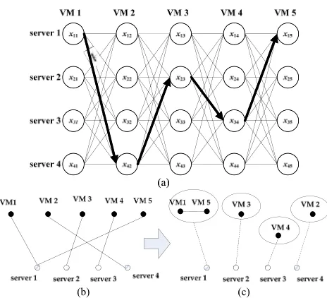
Fig. 1. (a) Example of a construction scheme, with N=5 and Mt= 4.

(b) Simplified bipartite graph of VMP, with solid lines representing VMs assigned to servers. (c) Grouping relationship graph of VMs in VMP. The ellipsoid represents a VM group onto a server. The solid line represents the link between VMs which are assigned on the same server. The dotted lines represent an assignment.

Dorigo and Gambardella [43] initially for solving the traveling salesman problem (TSP). Real ants are capable of finding the shortest path between the nest and the food source according to information passed via pheromone. Inspired by the foraging behavior of ants, ACS uses pheromone to record historical searching experience. Moreover, heuristic information is introduced to provide greedy information to guide the search. In solving a TSP, ants construct a solution by visiting the cities one by one until all are visited. During the construction process, the next city to visit is selected according to the pheromone and heuristic information. Similarly, a VMP can also use such a step-by-step con-struction as shown in Fig. 1(a), assigning the VMs one by one to suitable servers. Thus, ACS is applicable to VMP problems.

C. Pheromone in ACS

the link between VMs. Based on this consideration, we intro-duce pheromone between VM pairs to record the grouping relationship of VMs.

III. OEMACSALGORITHM FORSOLVING THEVMP

A. Initialization State Configurations

To minimize the number of active servers and then reduce the energy consumption for cloud computing, we develop an ACS-based approach here, with OEM operations. The resultant OEMACS algorithm searches for a solution with min-imal number of servers to host all the VMs. We denote this minimal number as Mmin in the feasible globally best solu-tion Sgb. Since Mmin is our optimization objective which is unknown in advance, we begin with Mmin = N in the

ini-tialization state, where N is the number of VMs. This means that the initial feasible globally best solution Sgb is to place the N VMs on N servers with one VM mapping to one server. For each pair VM k and VM j(j = k), we introduce a pheromone value τ(k,j) and initialize it as τ0 = (N)−1. The pheromone value indicates the preference of two VMs to be assigned to the same server according to the historical experience.

B. Solution Construction

After the initialization, OEMACS goes to construct solu-tions iteration by iteration so as to find better feasible solusolu-tions with fewer servers. In each iteration t(t ≥ 1), OEMACS aims to find a feasible solution with one server less than

Mmin. Therefore, the ant tries to place the N VMs to the

Mt=Mmin−1 servers.

In each iteration, multiple ants construct their own solu-tions (assignment) with the guidance of the construction rule. Each ant maintains a construction process by choosing ver-tices from a construction scheme. Fig. 1(a) shows an example of the construction scheme with N = 5 VMs and Mt = 4 available servers. It can be observed that the vertices of the construction scheme are arranged into an Mt×N matrix. Each vertex xijdenotes a VM assignment to a server. The undirected arc between two vertices in the adjacent columns indicates the potential route of ants. Taking Fig. 1(a) as an example, a solution S= {s1,s2,s3,s4},where si indicates a set of VMs assigned to server i, is constructed by the ant according to the path(x11,x42,x23,x34,x15)(denoted by black arrows line). This solution shows that all the four servers are active to host the five VMs, with the consolidation as s1= {1,5},s2= {3},

s3= {4},and s4= {2}.

Each ant adopts similar process to construct a solution according to the construction scheme like Fig. 1. Note that the VMs are randomly shuffled before each construction pro-cess. Then the ant constructs a solution by assigning VMs one by one to the servers. Therefore, the VMs are not in particular order for solution construction in the evolutionary process. We describe the solution construction process based on one ant in the follows. It should be noted that the following description is based on a partial solution under construction. There are totally N steps for an ant to construct a solution, with each step to select a proper server for the corresponding VM. In the

lth(1≤l≤N)step for placing VMj, a set of available servers

Ij is first defined as

Ij=

i

N

n=1

xin·vcn+vcj ≤PCi and N

n=1

xin·vmn

+ vmj≤PMi,1≤i≤Mt

(8)

whose element i stands for that server i has enough remain-ing resources (both CPU and memory) to host the unassigned VMj. Then the ant uses a state transition rule to select a proper server i from the set Ij. The pheromone and heuristic values in the state transition rule are described as follows.

For the pheromone, OEMACS deposits the pheromone between VMs rather than between a VM and a server. So we design a method to translate the pheromone between VM pairs into the preference between VM and server (the server here is also the existing VMs group which includes the links between VMs). The preference between VMj and server i rep-resents the historical experience of packing the VMj together with those VMs (the set of si) that have already been placed on server i. Suppose the pheromone between two VMs, VM

k and VMj, is denoted by τ(k,j). We calculate the pref-erence value T(i,j) of VMj to be assigned to server i as the average of the pheromone between VMj and the VMs that have been placed on server i. If there is no any VM deployed on server i, the value of T(i,j)is set asτ0. Therefore, we have

T(i,j)=

₁ |si|

k∈siτ(k,j), if |si| =0

τ0, otherwise

(9)

where si is the existing VM set on server i and |si| is the number of VMs deployed on server i.

Unlike the pheromone that provides historical information, the heuristic information is for deriving a better selection at the current local situation by a greedy strategy. In order to use a smaller number of active servers, each active server needs to host more VMs, which results in an increase of resource utilization of the server. On the other hand, the balance use of resources in all dimensions helps avoid the situation that some resources are highly utilized while other kinds are lowly utilized, which is not beneficial to the full use of the servers. Based on these, the heuristic information is designed to improve the utilization of different resources as well as to balance the usage of different resources in the servers (the utilization of different resources being high and similar). The heuristic information is associated to each VM assignment for measuring the utilization improvement that VM

j can bring to server i, whose value is calculated as

η(i,j)=

1.0−PCi−_PCUCi−vcj

i −

PMi−UMi−vmj

PMi

PCi−UCi−vcj

PCi

+PMi−UMi−vmj

PMi

+1.0

(10)

the denominator of (10); another is the balance of the remain-ing resources on the server, as the numerator of (10). The increase of the resource utilization and the balanced use of different resources benefit VM consolidation and then reduce the number of active servers.

With the design of pheromone and heuristic information, the probability for assigning an unassigned VMj to server i is calculated by

p(i,j)= T(i,j)η(i,j)

β

k∈IjT(k,j)η(k,j)β

, ∀i∈Ij (11)

where β(β > 0) is a predefined parameter that controls the relative importance of heuristic information.

In the OEMACS algorithm, the state transition rule is as follows: for VMj, it chooses server i from the servers set Ij by applying the rule given by

i=

arg max

k∈Ij

T(k,j)η(k,j)β,if q ≤q0

I, otherwise

(12)

where q is a random number uniformly distributed in [0,1],

I is a random number selected from Ij by a roulette wheel selection according to probability distribution in (11), and q0 is a predefined parameter (0 ≤ q0 ≤1) and is used to con-trol the exploitation and exploration behaviors of the ant. If q is not larger than q0, then the ant chooses the server whose preference value T and heuristic ηare maximal, measured by

T(i,j)η(i,j)β. Otherwise, the ant chooses server i which is probability selected according to (11).

A special case is that all servers are overloaded after join-ing VM j (i.e.,Ij = ϕ). To address this issue, we design a complementary rule to assign VMj to server i as

i=

arg min

1≤k≤Mt

over(k),if q≤q0

R, otherwise (13)

where R is a random integer in [1,Mt] selected by a roulette wheel selection according to the probability distribution in (15). If a randomly generated number q is not larger than q0,then the ant chooses the server whose overload rate after joining VMj is minimal. The overload rate describes the difference between the usage and the resource capacity after joining VMj. We calculate the overload rate over(i) of server i as

over(i)= PCi−UCi−vcj

PCi +

PMi−UMi−vmj

PMi .

(14)

Otherwise, VMj will be assigned to server i(1 ≤ i ≤ Mt) which is selected according to the probability distribution

r(i,j)=1−_Mover(i)

t

k=1over(k)

. (15)

C. Objective Function

After an ant has finished constructing a solution, we must evaluate its fitness value. Assume that S is an assignment

solution to the VMP problem. We evaluate the solution in a two hierarchical structure as

f1(S)= Mt

i=1yi,if S satisfies the capacity constraint

Mt+1, otherwise

(16)

f2(S)= Mt

i=1

_|

PCi−UCi|

PCi +

|PMi−UMi|

PMi ·

yi (17)

where Mtis the number of servers provided in current iteration

t,yi means that whether server i is used in the solution S. In (16), if the solution is feasible, f1(S)is the number of active servers, which is not larger than Mt.Otherwise, f1(S)is set to

Mt+1 to distinguish from the feasible solutions, which means that the number of servers we really need to use is the same as the best feasible solution in the last iteration, that is, equals to Mmin because Mt = Mmin−1. Equation (17) calculates the approximation of the placement to fill up the servers, to evaluate the resource utilization or distinguish the easiness of being transformed into a feasible solution. For two solutions, we compare their f1 values first, and select the solution with a smaller f1 value. If two solutions have the same f1 value, we compare their f2 values, then select the one with a smaller

f2 value. That is, the solution with fewer servers and higher utilization is preferred.

D. Pheromone Management

The pheromone records the historical preference informa-tion. A local pheromone updating and a global pheromone updating rule are implemented in the optimization process. After a solution has been constructed by each ant, the local pheromone updating operation is performed on each VM-pair

(k,j)on the same server. The updating rule is

τ(k,j)=(1−ρ)·τ(k,j)+ρ·τ0 (18) where 0< ρ <1 is the pheromone decay parameter.

In contrast, only is the best solution of the current iteration allowed to perform the global pheromone updating operation at the end of each iteration. When all the ants have built their solutions, the best solution of the current iteration can be found and denoted as Sb. The solution Sb, however, can be either feasible or infeasible. If Sbis feasible, it means that OEMACS has found a new feasible solution with servers no more than

Mt, then we update the feasible globally best solution Sgb to

Sband update Mmin to f1(Sb).That is, the active servers used in the solution Sb. On the other hand, if Sb is infeasible, it means that OEMACS cannot find a feasible solution with only

Mt servers. In this case, OEMACS carries out the OEM local search on Sb, which is described in Section III-E. No matter the Sb is feasible or not, the global pheromone updating rule is carried out on Sbafter the above operations, to increase the pheromone on the VM-pair of the same server of Sb _as

τ(k,j)=(1−ε)·τ(k,j)+ε· τi,if(k,j)∈si,∀si∈Sb (19)

τi = 1

f1

Sb+

1 LCi+LMi+1.

Fig. 2. Example of the ordering exchange operation on a solution where server 1 is overloaded while servers 2–4 are not overloaded, and the solution becomes feasible after exchanging VM 11 on server 1 with VM 7 on server 4.

where ε(0 < ε < 1) is the pheromone enhance parameter,

f1(Sb)is the number of servers used in Sb,LCi and LMi rep-resent the normalized remaining CPU and memory resource of server i (the ratio of remaining resource to the total resource). The key idea behind the above equation is to record an almost “full” VM group (the utilization of server is high) and a better solution. The pheromone of VM pairs in the more “occupied” server will increase more.

The local and global pheromone updating rules play dif-ferent roles in guiding the search act of the ants. The local pheromone updating rule reduces the appeal of grouping VM pair which has been found by the last ant, and to help the other ants explore new assignment space. It is able to avoid rapid convergence toward a narrow neighbor region of the best previous route and enhance the population diversity. Global pheromone updating rule is used to strengthen the ties between VM pairs in the good assignments and guides the ants to construct better solutions in a more promising direction.

E. Local Search Procedure

Local search is significant in transforming an infeasible solution into a feasible solution. At the end of each iteration, before the global pheromone updating, the OEM local search is carried out on the current best solution Sb _{if S}b _is infea-sible. The OEM includes two procedures. First, an ordering exchange operation and then a migration operation. Both oper-ations try to adjust the VM assignments to ease or eliminate the overloaded servers. If Sb becomes feasible after the local search, we update the feasible globally best solution Sgb to

Sb and update Mmin to the server number of the new feasible solution.

1) Ordering Exchange Operation: The ordering exchange

operation swaps VMs between different servers. The operation is used to enhance the resources utilization of nonoverloaded servers and to avoid unbalance resources utilization of over-loaded servers. For each overover-loaded server, we can try to exchange every VM on it with every VM on a nonoverloaded server, to observe whether the overloaded server can become nonoverloaded while the nonoverloaded server is still nonover-loaded. In order to reduce the computational burden of this process, we design the following exchange strategy.

For every overloaded server i, we sort the VMs on it according to the absolute difference between CPU and RAM requirements and give preference to the VM with higher dif-ference for exchange (i.e., sort to front). Then we select one nonoverloaded server k for exchange. The VMs on server

k are sorted by the rule contrary to server i (i.e., VM with

smaller resource difference is sorted to front). Subsequently,

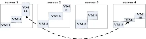
Fig. 3. Example of the migration operation where VM 1 on server 1 is moved to server 3. The dotted rectangular with VM number represents a VM, and the large solid rectangular represents a server.

we check the VMs on server i one by one with the VMs on server k one by one to determine whether the two VMs can be exchanged. The process ends until the exchange makes server

i become nonoverloaded while the server k is still

nonover-loaded, or all VMs on server k have been checked whether to exchange. If server i cannot turn to nonoverloaded after all exchange attempts, another nonoverloaded server is selected for exchange.

Fig.2presents possible transition directions of the exchange operation in an example. The dotted rectangular with VM number represents a VM, and the large solid rectangular rep-resents a server. The length of horizontal line of rectangular represents CPU size, and the length of vertical line represents the RAM size. Two VMs connected by arrow line are the exchange objects. Server 1 is overloaded because the required RAM exceeding the size. Servers 3 and 4 are not overloaded. After the ordering exchange operation, VM 11 on server 1 is exchanged with VM 7 on server 4. Then the solution becomes feasible. The exchange makes the resource utilization be less than or get near to the resource upper bound of servers.

2) Migration Operation: The migration operation

sched-ules a VM from an overloaded server to a nonoverloaded server that has enough remaining resource to satisfy the resource requirement of this VM. The operation is similar to Falkenauer’s remove mutation [57]. Check the VMs on the overloaded servers one by one with the nonoverloaded servers one by one to determine whether the VM can move to the server. The operation terminates when all servers become nonoverloaded or there is no VM movement that can be car-ried out. A possible transition scenario of migration operation is illustrated in Fig.3. The length of horizontal line of rect-angular represents CPU size, and the length of vertical line represents the RAM size. The pale VM 1 on server 3 shows that VM 1 fits server 3. The arrow line connects a VM and a server, which highlights the direction of VM migration.

Local search is based on the idea of lowering resource utilization of overloaded servers. The migration operation is performed after the ordering exchange operation. In an early stage, the number of servers is large enough to find a feasible solution, so local search does not work. In a later stage, the searching approaches the optima and becomes harder. Local search can improve searching by converting the infeasible solution into a feasible one.

F. Complete OEMACS Algorithm

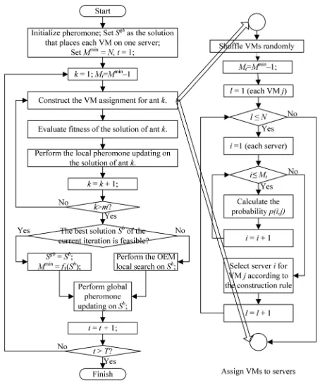
The overall flowchart of the OEMACS algorithm is shown in Fig.4and is described in the following six steps.

Fig. 4. Flowchart of the OEMACS algorithm.

on N servers with one VM mapping to one server. Therefore, set the number of minimum servers

Mminas N. Set the iteration t=1.

Step 2: Set Mt=Mmin−1.Let m ants construct m solutions according to the construction rule, and perform local pheromone updating on each solution. Step 3: Evaluate the fitness values of the m solutions. Step 4: Find out the current iteration best solution Sb; if

Sb is feasible, update Sgb as Sb and set Mmin =

f1(Sb);otherwise, perform OEM local search on Sb. Update Sgb and Mmin if the local search successes. Step 5: Perform global pheromone updating on Sb. Step 6: Termination detection. When the maximum number

of iterations is reached, the algorithm terminates. Otherwise, set t=t+1 and move to step 2 for the next iteration.

Throughout the procedure, step 2 is a main process of the OEMACS algorithm. A detail description is shown in the subflowchart in Fig.4.

IV. EXPERIMENTS ANDCOMPARISONS

Experimental tests are carried out in this section to verify the performance of OEMACS. All the algorithms have been implemented in C+ +,and ran on a PC with a Pentium Dual CPU i7 and 4.0GB RAM.

The experiment instances in [32] are used to test the performance of the OEMACS algorithm. Moreover, we design two other test sets, tests B and C, with a bottleneck resource (one resource demands more) under homogeneous and het-erogeneous server environments, respectively. The efficiency

of OEMACS is also evaluated by comparing with the corre-sponding results obtained by the FFD heuristic approach [40], the RGGA approach [32], the ACO-based approach [11], multiobjective MACO [36], and HACOPSO [37]. FFD sorts the VMs in descending order by first considering CPU require-ment and then RAM requirerequire-ment and assigns each VM to the first server with enough remaining resource. FFD gives the result which is less than or equal to 11/9∗OPT+1,and per-forms well compared with other deterministic algorithms [40]. Therefore, FFD can be regarded as a representative of heuris-tic and determinisheuris-tic algorithms. The RGGA is compared because of its superiority over traditional approaches [32]. In an RGGA, a crossover operator is performed to generate a candidate solution. The servers in two parents are combined together and sorted by resource utilization. Then, the more full servers with different VMs are selected. The remaining unassigned VMs are sorted in a decreasing order accord-ing to the requirement of CPU first and then memory, and are placed by the FFD strategy. The ACO algorithm based on max-min ant system in [11] is compared to verify the efficiency of the proposed ACS approach. The MACO and HACOPSO are compared because they are the most recent well-performed approaches that are reported to have bet-ter performance than other algorithms, so as to evaluate the performance and advantages of OEMACS.

The OEMACS related parameters are m = 5, q0 = 0.7,

ρ =0.1, = 0.1, β =2.0, M1 =N−1, τ0 = (N)−1, and maximal iteration T =50. We assume that the resource uti-lization can reach 100%. Parameter settings of RGGA, ACO, MACO, and HACOPSO are consistent with their original lit-eratures, with their population sizes being 75, 5, 8, and 20, respectively, while their maximal iterations are 100, 50, 100, and 500, respectively. Therefore, the maximal function eval-uations (FEs) for RGGA, ACO, and MACO are 7500, 250, 800, and 10 000, respectively. Therefore, RGGA, MACO, and HACOPSO all have much larger FEs than the one used by OEMACS, which is only 5×50=250,because we anticipate that OEMACS converges faster. As EC algorithms all con-tain cercon-tain randomness in the search process, they perform 30 independent runs on each instance in all the test environ-ments for fair comparison. The runtime of FFD is a few micro seconds in all instances. So it is not listed. The best results are marked in bold face.

A. Test A: Large-Scale Homogenous Environment

TABLE I

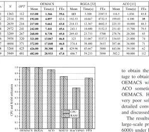
EXPERIMENTALRESULTCOMPARISONS INTESTA WITHDIFFERENTSIZE OFVM

Fig. 5. Average utilization of CPU and RAM of all active servers on A9.

in the table represents the minimal number of servers used for deploying all the VMs.

It can be observed from Table I that OEMACS obtains the best solution. More significantly, OEMACS obtains the same number of active servers in 30 runs, indicating its sta-ble performance. The FFD yields very poor solutions using the maximal number of servers. ACO, and MACO always perform worse than OEMACS and RGGA but better than FFD. HACOPSO performs better than FFD on some cases. Moreover, as the problem size increases, the advantages of EC-based algorithms become more significantly when com-pared with the traditional algorithm FFD. For example, in A1, ten physical servers are less in OEMACS than in FFD, while in A9, more than 100 physical servers are less. Fig. 5 dis-plays the utilization of CPU and RAM of active servers for OEMACS, RGGA, ACO, MACO, HACOPSO, and FFD on A9. OEMACS and RGGA obtain the highest CPU and RAM utilization which is near to 100%. More significantly, the utilization rates of the CPU and RAM resources are balanced. Another advantage of OEMACS is that it can obtain better solution than other approaches do with fewer FEs in much shorter computational time. Table I records the average run-ning time and FEs when the algorithm cannot improve the solution quality any more. For example, in A1, OEMACS uses average 39.6 FEs (with average 1.366 s) to obtain the final result 113. However, when RGGA stops in the result 113, it needs average 2387.5 FEs (with average 3.300 s), and ACO needs 45.8 FEs (with 1.836 s) to obtain the result 116.5, MACO needs 285.6 FEs (with 11.200 s) to obtain the result 130.26, and HACOPSO needs 914 FEs (with 7.233 s)

to obtain the result 117.56. The convergence speed advan-tage to obtain good result is very significant when compared OEMACS with RGGA, MACO, and HACOPSO, although ACO sometimes stops improving the solution early than OEMACS. However, the early stop makes ACO result in very poor solutions, especially in large-scale problems. The detailed convergence of OEMACS will be further analyzed and discussed in Section IV-E.

The results in test A show that OEMACS is able to solve large-scale problems (even with number of VMs up to about 6000) under homogenous server environments where the rel-ative overall demands of CPU and RAM are comparable (the ratio being 1:1). Moreover, OEMACS has general better performance in obtaining better solution with fast convergence speed when compared with the compared FFD, RGGA, ACO, MACO, and HACOPSO algorithms.

B. Test B: Bottleneck Resource Homogenous Environment

To further test the effectiveness and efficiency of OEMACS, we designed a set of data that models the VMs and servers in a cloud computing environment that has bottleneck resource. We created eight different problem instances with different sizes from 100 to 2000, numbered sequentially from B1 to B8. Each server has a 16-core CPU and 32GB RAM. Each VM has CPU requirement of 1–4 cores and memory require-ment of 1–8GB, which is generated randomly from discrete uniformly distributions. CPU is the bottleneck resource in this case because the probability of 4-core VM is 0.25 but 7 or 8GB VM is 0.125. Therefore, the overall ratio of requirement of CPU to memory utilization is nearly 10:9. Since the instances are generated randomly, we do not know the optimal solu-tion. We estimate the lower bound of the optimum as M and˜

calculate its value as

˘

M=max

N

j=1vcj PCi

,

N

j=1vmj PMi

(21)

where PCi and PMi are the CPU and RAM capacities of any server because the servers are homogenous, while N_j=1vcj andN_j=1vmjare the sum of CPU and RAM requirements of all the VMs, respectively.

The results obtained by OEMACS, FFD, RGGA, ACO, MACO, and HACOPSO are given and compared in Table II. Similar to the results in test A, results presented in Table II

TABLE II

EXPERIMENTALRESULTCOMPARISONS INTESTB

TABLE III

EXPERIMENTALRESULTCOMPARISONS INTESTC

Fig. 6. Average utilization of CPU and RAM of all active servers on B8.

be observed that FFD cannot find the optima in all instances and performed the worst compared with other five algorithms. OEMACS not only outperforms FFD, but also does better than RGGA, ACO, MACO, and HACOPSO. From TableII, we can see that RGGA and ACO achieve results that are equal toM inˇ

only two out of the eight instances whose number of VMs is not larger than 200. However, the proposed OEMACS obtains results that are equal toM in all of the eight instances withinˇ

only 30 FEs. When the problem size increases, the superior-ity of OEMACS is more apparent. In comparison with ACO, the advantage of OEMACS is obvious. ACO cannot always obtain the optima within the predefined maximum number of FEs except for very small size instances like B1 and B2. For instance B1, ACO is very fast to find the optima in the second iteration while OEMACS in the fourth iteration. This may be due to that ACO selects VM to be assigned to the current server and open another server while no VM can be assigned to it. ACO acts like the greedy algorithm FFD and can find good solution in early stages to converge quickly in very small size problems. OEMACS constructs solutions from VM’s view and selects a server for each VM, so it converges a litter slow in early stage and but jumps out of local optimal rapidly. The results show that OEMACS outperforms not only tradi-tional FFD and RGGA, but also other ACO-based algorithms,

in terms of both solution quality and the optimization speed, especially in large-scale homogeneous server problems with bottleneck resource.

Fig. 6 shows the average CPU and RAM utilization of the active servers in the assignment obtained by OEMACS, RGGA, ACO, MACO, HACOPSO, and FFD on test B8. OEMACS obtains the largest CPU and memory utilization. The CPU (the most critical resource) utilization is near to 100% and RAM is near to 90%. It shows that different resource-intensive VMs are balanced, so that both resources are better exploited. In general, OEMACS is able to obtain the best assignment.

C. Test C: Hard Heterogeneous Environment

In tests A and B, all the servers are homogeneous, as in real cloud environment servers are often heterogeneous. So we designed another test environment with heterogeneous servers and CPU-intensive and RAM-intensive VMs. Two kinds of servers (type s0 16-core CPU, 32GB RAM, Pmax = 215 W and type s1 32-core CPU, 128GB RAM, Pmax=300W)are provided. The number of servers of type s0 is set as Ms0 = 9N/10 (N is the number of VMs) and type s1 as Ms1 =

N/10.This makes that using only the large servers (e.g., type

s1) cannot host all the VMs, so that both types of servers have

to be used. We created five problem instances of different sizes from 100 to 500, which are numbered sequentially from C1 to C5. In every problem instance, VMs are generated by discrete uniform distribution of [1, 8] for CPU and [1, 32] for memory. The memory is the bottleneck resource. The lower bound of the optimum M is estimated as˜

˘

M =Ms1+max N

j=1vcj−PCs1·Ms1 PCs0

,

N

j=1vmj−PMs1·Ms1 PMs0

(22)

Fig. 7. Average utilization of CPU and RAM of active servers of all, types s0 and s1 on C5.

The results are given in Table III. As shown in the table, FFD performs poorly. Neither can RGGA, ACO, MACO, nor HACOPSO find the optima in all instances. In contrast, OEMACS can obtain the best results among all the six algo-rithms in all instances and can even find the optima in C2, C3, and C5. In the instances C1 and C4, the results obtained by OEMACS are only with one server away from the optima. However, the results obtained by other algorithms are far away from the optima. Moreover, OEMACS finds the optima within 250 FEs while RGGA and other ACO-based algorithms cannot find even using more FEs. In summary, OEMACS outperforms FFD significantly in terms of solution quality and outper-forms RGGA and other ACO-based algorithms in terms of both solution quality and search speed.

Fig.7shows the average CPU and memory utilization of the active servers of all, types s0 and s1, respectively, in the assign-ment obtained by different algorithms. Both average CPU and RAM utilization of all active servers of FFD’s assignment are the lowest. There is a significant gap between the utilization of CPU and RAM both for types s0 and s1, which demon-strates that FFD cannot efficiently balance different resource. For OEMACS, the CPU utilization of the active servers of type

s0 is the highest, while type s1 is smaller than the RGGA. It

shows that the OEMACS prefers to highly integrate the VMs on high configuration servers while RGGA prefers low-profile servers. Memory is the bottleneck resource and limits the con-solidation level. The average memory utilization of OEMACS is the highest, near to 100%, which shows that OEMACS can obtain the highest consolidation of VMs with high resource utilization.

Compared with test B, OEMACS needs more FEs and time to obtain the optima of the same problem size. This is because the VMP problem becomes harder in heterogeneous server environments. However, OEMACS can still find the optima by using more computing power. Take C5 for exam-ple, OEMACS can still achieve the optima of 500 VMs within 0.5 s. OEMACS can find the optima in acceptable time. FFD does not seem suitable for large-scale problems as it performs poorly. OEMACS performs well in all three tests. Tests A and B are in homogeneous server environments with different cor-relation ratios for CPU and memory utilization, and test C is of a heterogeneous server environment. Therefore, our results

TABLE IV

COMPARISONRESULTS ONSTATISTICALLYSIGNIFICANTDIFFERENCES

OFOEMACS WITHALLCONTENDERS AND ONRUNTIME OFALL

ALGORITHMS INTESTSA, B,ANDC

show that OEMACS can find optima or quasi-optimal solu-tions for large-scale homogeneous and heterogeneous server data center environments with resource-intensive VMs.

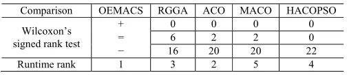
A nonparametric statistical test called Wilcoxon’s signed rank test is conducted between the compared algorithm and OEMACS at a 5% significance level to judge whether the results obtained with the best performing algorithm signifi-cantly exhibits superior performance. The null hypothesis in each test is that no difference exists between the compared algorithm and OEMACS. We mark the cases with “+” and “−” when the null hypothesis is rejected to indicate that the compared algorithm performs significantly better or worse than OEMACS. The cases marked “=” means that there is no statistically significant difference between the performance of the two algorithms. The numbers of the three kinds of statisti-cal significance cases(+/=/−)are reported in TableIVin this paper and the details in each test are listed in Table S.I in the supplementary file. From the table, we can see that OEMACS performs significantly better than RGGA, ACO, MACO, and HACOPSO on 16, 20, 20, and 22 out of 22 cases, respectively. OEMACS is seen outperforming the algorithms compared.

The runtime required to obtain the best solution for each algorithm (whose mean value has been reported in TablesI–III) is also performed with a t-test at a 5% signifi-cance level to compare with the one of OEMACS. The results of t-value and p-value are reported in Table S.II in the supple-mentary file. From Table S.II, we can see that OEMACS can find better or similar solutions in significantly shorter time in most cases. Although both number of FEs and runtime that are required to obtain best solutions can reflect the convergence speed of the algorithm, it is still interesting to investigate the total runtime of the algorithm until it terminates. Therefore, the mean total runtime of the 30 runs are presented and com-pared in Table S.III in the supplementary file, for each problem instance and for each algorithm. Table IV also reports the total runtime ranks of OEMACS, RGGA, ACO, MACO, and HACOPSO. From the table, we can observe that the runtime of OEMACS ranks the first and is the shortest among the compared algorithms.

TABLE V

COMPARISONRESULTSBETWEENOEMACSANDCPLEX

(a) (b)

(c) (d)

(e)

Fig. 8. Influence of the parameters in OEMACS on A1 and C5. (a) m. (b) q0.

(c)β. (d)ρ. (e) .

400 VMs (where CPLEX stops when it obtains the results due to out-of-memory). On the running time, OEMACS is much faster than CPLEX. The speed advantage becomes more evident as the problem scale increases. Moreover, CPLEX con-sumes too much time when dealing with VMP with more than 500 VMs, indicating that it may be not suitable for large-scale VMP. Therefore, we only give the available results on B1–B4 and C1–C4 in Table V.

D. Analysis of OEMACS Parameters

The OEMACS parameters include the population size of ants m, β,q0, ρ,and . In order to study the influences of the parameters to the solution quality, we take A1 and C5 as an example and perform parameter analysis in this section.

The investigation begins with the parameter m. We set m from 5 to 50 with a step length of 5. All the other parameters remain the same as stated above. Both the mean results of A1 and C5 plotted in Fig. 8(a) are nearly invariant with the increase of population size m. Nevertheless, a large population size causes a high computational burden in each generation.

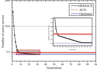
Fig. 9. Convergence curves of OEMACS and ACO on A9.

By considering both of these, this paper adopts the population size of 5 in OEMACS.

The next parameter tested is q0. In the following investi-gation, q0 varies from 0.1 to 0.9 with a step length of 0.1. The mean number of active servers in obtained solutions are plotted in Fig.8(b). The tendency of the curves indicates that it is better to use a larger q0for better performance. However, too large a q0makes the algorithm perform poorly due to the loss of exploration ability, e.g., the results for q0 = 1.0 are too bad to be plotted within Fig. 8(b). Therefore, we set q0 0.7 in this paper.

Then parameter β is investigated. As shown in Fig. 8(c), for A1, the performance of OEMACS with different configu-rations is similar. For C5, whenβ is 2, 5, 6, or 9, OEMACS performs the best. The results forβ =0 are poor and not plot-ted in Fig.8(c), which indicates that the heuristic information plays an important role on the algorithm performance.

Finally, parameterρfor pheromone local updating and for global updating are tested. Fig.8(d) and (e) shows the results obtained. The results are poor when parameters ρ and are set to 0 or 1.0; so they are not plotted in Fig. 8(d) and (e). For A1, the performance of OEMACS is similar with different values of ρ, while for C5, a relatively small ρ value seems to be preferred. This may be due to the fact that a smaller

ρ is helpful to avoid a too rapid pheromone evaporation on the visited assignment and to use the historical experience recorded in the pheromone. The curves in Fig. 8(e) of the impact of are nearly parallel to the horizontal axis. OEMACS is seen insensitive to the value of .

From Fig. 8, the impact of β, ρ, and further confirms that these parameters are promising and OEMACS is not very sensitive to the parameters. This is also an advantage of the OEMACS algorithm.

E. Further Convergence Analysis of OEMACS

(a)

(b) (c)

Fig. 10. Experimental results of OEMACS and its variants, noPhe, noHeu, noPhe&noLS, noHeu&noLS, and noLS on A9. (a) Convergence curves with error bars. Box plots of results at (b) 30 generations and (c) 50 generations.

and surpasses ACO, before slowing down when approaching the optima (with 481 servers) from the fifth iteration, and then converging to 482 at the 30th iteration. Conversely, starting on lower server numbers initially, ACO undergoes an incremental progress, and converges prematurely to a higher level (resulting in 502 servers).

The above results demonstrate that OEMACS can converge to a near-optima more effectively and more quickly.

F. Benefits of Pheromone and Heuristic Components

We are interested in identifying the benefit of the three components of OEMACS: 1) pheromone; 2) heuristic infor-mation; and 3) local search. For this purpose, we consider five OEMACS variants, i.e., noPhe, noHeu, noPhe&noLS, noHeu&noLS, and noLS. They differ from OEMACS only in that noPhe does not use the pheromone (and “preference”), noHeu does not adopt the heuristic information (β = 0), and noLS does not perform local search. The A9 is taken as an example. The convergence curves and box plots of results are illustrated in Fig. 10. Experimental results have shown that both the pheromone and heuristic information are fundamental in helping the OEMACS algorithm find good solutions within a reasonable period of time. As seen from Fig. 10(b) and (c), the noPhe variant and noPhe&noLS vari-ant have similar but poor performance. This is because that heuristic information and local search are greedy strategies and therefore the OEMACS variants without pheromone are actually reduced to a stochastic restart greedy algorithm that is easy to be trapped into local optima. Moreover, noHeu per-forms better than noPhe, likely due to that it is guided by reinforcements provided by the global updating rule in the form of pheromone although noHeu is not helped by heuris-tic information. Therefore, pheromone plays a significant role in enhancing the algorithm performance, helping OEMACS perform better than a randomized restart greedy algorithm.

When referring to the heuristic component, the results show that the performance of noHeu&noLS is worse than both noLS and noHeu, while all these three variants perform significantly worse than OEMACS. These indicate the importance of both the heuristic information and local search in enhancing the algorithm performance. From Fig.10(a) and (b), we can see that OEMACS converges to solution with 482 servers within 30 generations while its noHeu variant gets significantly worse solution with 504 servers. Even given more computational budget (50 generations), noHeu still cannot obtain solution of 482 as illustrated in Fig. 10(c). Along the whole con-vergence process, OEMACS always keeps its result below noHeu, especially with a large difference in the early stage. Similarly, noHeu&noLS also performs worse than noLS. Thus, the heuristic information helps speed up the convergence and improves the performance of the algorithm.

G. Effectiveness of Local Search

Local search is an important feature in the proposed OEMACS. Two operations of local search contribute in dif-ferent ways to the optimization process. In this section, we validate the effectiveness by comparing the results of OEMACS with its variants without local search or with only one operation of local search. The variants without local search, ordering exchange operation or migration operation are termed noLS, noE, and OEMACS-noM, respectively. The settings of these variants are exactly the same as OEMACS except that one of the three com-ponents is not applied. The following study takes A2, B8, and C5 as examples. A2 and B8 are large-scale problems of homogeneous server settings, and C5 is a complex problem in a heterogeneous server environment. The situations on the other problems are similar.

Table VI lists the results of the four algorithms averaged over 30 independent runs. It can be observed that OEMACS obtains the best solutions, followed by OEMACS-noM and OEMACS-noE, whereas OEMACS-noLS performs the worst. The OEMACS-noLS and OEMACS-noE cannot achieve the optima or approximate optima in 7500 FEs. The advantages of OEMACS over the other three algorithms confirm that the local search is indeed effective in finding high-quality solutions. Compared with the migration operation, the order-ing exchange operation contributes more in improvorder-ing the solutions since OEMACS-noM can find good solutions as OEMACS using more FEs while OEMACS-noE cannot within the maximum FEs.

TABLE VI

EXPERIMENTALRESULTCOMPARISONS OFOEMACS, OEMACS-NOM, OEMACS-NOE,ANDOEMACS-NOLSFORPROBLEMA2, B8,ANDC5

TABLE VII

SUCCESSRATE OFIMPROVING THEINFEASIBLESOLUTION

OFLOCALSEARCH ONA2, B8,ANDC5

For C5, the solution, which is transformed by the ordering exchange operation can be improved by the migration opera-tion. This helps the exchange operation to improve the solution further.

For B8, the ordering exchange operation improves all the infeasible solutions on B8, so the migration operation is not executed, and OEMACS performs the same as OEMACS-noM. The time of OEMACS and OEMACS-noM is close.

For A2, the success rate of the ordering exchange operation is just 88.60%; so the migration operation is involved. The migration operation does not transform infeasible solutions into feasible solutions. However, the migration effect results in pheromone transmitting the VM group information into the next generation. Thus the migration operation improves the algorithm indirectly. OEMACS converges in 42.6 FEs with 4.097 s, while OEMACS-noM in 45 FEs with 4.760 s, which shows that the migration operation leads to shorter time.

As for C5, although the success rate of the migration oper-ation is only 9.57%, it helps the algorithm converge more quickly. OEMACS uses only less than a half time to obtain the final results when compared with OEMACS-noM (i.e., 0.4526 versus 1.0). Moreover, the migration operation per-forms better when it cooperates with the ordering exchange. For all three problem instances, OEMACS takes the shortest time. Hence, both the ordering exchange operation and the migration operation are important for improving the solutions and finding the optima in shorter time.

All the results in Tables VI and VII indicate that local search is important and necessary in the proposed algorithm OEMACS.

H. Energy Saved by OEMACS

The benefit of consolidation is determined primarily by the amount of power wasted due to the resource underutiliza-tion. The power consumed by active but idle servers, that is, the quantity Pidle, is the major source of energy waste. The value of Pidle is expressed as a percentage or fraction

k of the power consumed when the server operates at full

capacity, Pidle = kPmax in (7). Pidle is an inherent part of

power consumption of an active server. For the given VMs, the utilization of CPU is determinant, so the second term

u·(1−k)Pmax in (7) is certain to be included in the power consumption. To reduce it, let us start with the first term

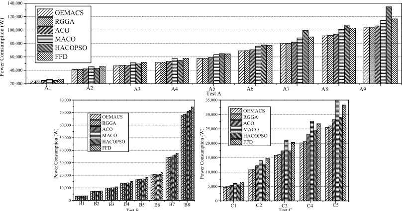
kPmax of (7). The Pidle is consumed only if the server is active. By means of consolidation to increase the resource utilization and reduce the number of active severs, the power energy can be significantly reduced. The Pmaxis set to 215W in tests A and B. Fig. 11 shows the power consumption of OEMACS, RGGA, ACO, MACO, HACOPSO, and FFD on tests A, B, and C, when k = 0.6. We can observe that OEMACS consumed less power than other algorithms in all cases. To further analyze the benefit of consolidation, we cal-culate the power consumption with different values of k in two scenarios with or without bottleneck resource. The following study takes A9 and B8 as examples. Both A9 and B8 are large-scale problems of homogeneous server settings, while B8 encounters bottleneck resources. The situations encoun-tered by the other problems are similar. Fig. 12displays the overall amount of power consumption of various algorithms on A9 and B8.

In Fig. 12(a), the consumed power of different algorithms for A9 is illustrated. Compared with FFD, OEMACS allows the data center to reduce the consumed power significantly, from about 9–15 kW. OEMACS and RGGA consumed the least power. In A9, the overall demands on the CPU and RAM are approximate. Both the utilization of CPU and RAM of OEMACS are incredibly closed to the permitted thresh-old (100%) seen from Fig.5. Different resources are utilized effectively. The consolidation of VMs allows the idle servers to be hibernated so as to reduce the consumed power. As the value of k increases, the reduced power increases.

Fig. 11. Power consumption of different algorithms under different test cases.

(a) (b)

Fig. 12. Consumed power with different values of k (the ratio of power consumed at idle state to maximum utilization) on (a) A9 and (b) B8.

FFD. The results in Fig. 12 confirm that OEMACS have a substantial advantage in saving power.

V. CONCLUSION

Energy consumption contributes most to the total cost in a cloud system. This motivates us to have developed an energy efficient OEMACS for VMP in cloud computing. The optimal VM deployment has been achieved with the minimum number of active servers and by switching off the idle servers.

The VMP problem is a complex NP-hard problem. To solve this problem, OEMACS, an ACS-based approach, has been developed in this paper. The assignment of VMs is constructed by artificial ants based on global search infor-mation. OMEACS distributes pheromone between VM pairs, which represents a bond among the VMs on the same server and records good VM groups through learning from histor-ical experience. To revise infeasible solutions, local search is performed, which contributes significantly to improving the solutions and speeding up global convergence of the OEMACS. Moreover, the number of servers provided for plac-ing VMs reduces as the generation number grows, avoidplac-ing possible wastes of computation while providing guidance for further advancement of the solutions. These distinct features and the strong global search nature of an ACS make the

OEMACS efficient for large-scale problems. It shows a sig-nificant advantage compared with other heuristic algorithms, which often encounter difficulties when the problem scale grows with cloud computing.

The OEMACS is applied to cloud systems of various sizes and characteristics. Experimental results show that OEMACS has achieved the objectives of minimizing the number of active servers, improving the resource utilization, balancing different resources, and reducing power consumption. Moreover, the parameter analysis shows that the performance of OEMACS is not very sensitive to the parameters, and this makes the OEMACS more competitive. In conclusion, the OEMACS is seen an effective and efficient approach to the VMP problem.

REFERENCES

[1] I. Foster, Y. Zhao, I. Raicu, and S. Y. Lu, “Cloud computing and grid computing 360-degree compared,” in Proc. IEEE Grid Comput. Environ. Workshop, Austin, TX, USA, 2008, pp. 1–10.

[2] Z.-G. Chen, K.-J. Du, Z.-H. Zhan, and J. Zhang, “Deadline constrained cloud computing resources scheduling for cost optimization based on dynamic objective genetic algorithm,” in Proc. IEEE Congr. Evol. Comput., Sendai, Japan, 2015, pp. 708–714.

[3] H.-H. Li, Y.-W. Fu, Z.-H. Zhan, and J.-J. Li, “Renumber strategy enhanced particle swarm optimization for cloud computing resource scheduling,” in Proc. IEEE Congr. Evol. Comput., Sendai, Japan, 2015, pp. 870–876.

[4] A. Q. Lawey, T. E. H. El-Gorashi, and J. M. H. Elmirghani, “Distributed energy efficient clouds over core networks,” J. Lightw. Technol., vol. 32, no. 7, pp. 1261–1281, Apr. 1, 2014.

[5] Z. H. Zhan et al., “Cloudde: A heterogeneous differential evolution algo-rithm and its distributed cloud version,” IEEE Trans. Parallel Distrib. Syst., 2016, to be published, doi: 10.1109/TPDS.2016.2597826. [6] X.-F. Liu, Z.-H. Zhan, J.-H. Lin, and J. Zhang, “Parallel differential

evolution based on distributed cloud computing resources for power electronic circuit optimization,” in Proc. Genet. Evol. Comput. Conf., Denver, CO, USA, 2016, pp. 117–118.