Quantum state comparison amplifier with feedforward state correction

PROCEEDINGS OF SPIE

SPIEDigitalLibrary.org/conference-proceedings-of-spie

Quantum state comparison amplifier

with feedforward state correction

L. Mazzarella, R. J. Donaldson, R. J. Collins, U.

Zanforlin, G. Tatsi, et al.

L. Mazzarella, R. J. Donaldson, R. J. Collins, U. Zanforlin, G. Tatsi, G. S.

Buller, J. Jeffers, "Quantum state comparison amplifier with feedforward state

correction," Proc. SPIE 10674, Quantum Technologies 2018, 106741D (21

May 2018); doi: 10.1117/12.2307818

Quantum State Comparison Amplifier with Feedforward

State Correction

L. Mazzarella

_{, R. J. Donaldson}

_{, R. J. Collins}

_{, U. Zanforlin}

_{, G. Tatsi}

_{, G. S. Buller}

_{, and J.}

Jeffers.

a

_{Department of Physics, University of Strathclyde, John Anderson Building, 107 Rottenrow,}

Glasgow G4 0NG, U.K.

b

_{Institute of Photonics and Quantum Sciences, School of Engineering and Physical Sciences,}

David Brewster Building, Heriot-Watt University, Edinburgh EH14 4AS, U.K.

ABSTRACT

Quantum mechanics imposes stringent constraints on the amplification of a quantum signal. Deterministic amplification of an unknown quantum state always implies the addition of a minimal amount of noise.1 _Linear

and noiseless amplification is allowed in principle provided that it only works probabilistically23 _{. Here we}

present a probabilistic amplifier that combines two quantum state comparison amplifiers (SCAMP)4 _together

with a feed-forward state correction strategy. Our system outperforms the unambiguous state discrimination (USD)5 _{measure-and-resend based amplifier in terms of the success probability-fidelity product and requires a}

no more complex experimental setting.

Keywords: quantum amplifier, state amplification, coherent states, state comparison, probabilistic amplifier, quantum technologies, optical amplifier.

1. INTRODUCTION

The efficient amplification of weak coherent states is important for the implementation of various quantum information processing tasks. For example, weak coherent states are used to encode information in quantum communications protocols such as QKD678∗ _{and QDS}1213_.

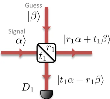
SCAMP is a mature technique that provides approximate probabilistic amplification for a known, symmetric set of coherent states by comparing at a beam splitter the unknown input state with a guess coherent state. The state comparison is shown in figure1: Alice picks one state form the set at random and provides it to Bob whose task is to amplify it. Bob does so by mixing it with the guess coherent state at the beam splitter in an attempt to achieve destructive interference in one of the arms, monitored by a single-photon avalanche diode (SPAD).14

From here on, we assume that the state space comprises two states {|+αi,|−αi}. Higher state spaces are possible but represent an additional degree of complication that we do not need here. Let us also assume that Bob chooses _|β1i = |+_rt1₁αi for his guess. If Alice’s input is |αi there will be destructive interference in the detector arm, preventing it from registering an event. In this case we say that Bob’s guess was right and the output will be given by the amplified state_|α

r1i(see the appendixAfor the detailed calculations of the coherent

amplitudes). The device gain is thus given by g2 ₌ 1

r2

1 Note that the gain of the system is linked to the beam

splitter parameters. On the other hand, if Bob’s guess is incorrect (i.e. _|−t1

r1αi) a non-zero coherent amplitude

will be incident on the detector and may or may not cause it to fire. The indication is imperfect because the lack of counts can be be due either to the imperfect efficiency of the detector or the non-zero overlap of the coherent state with the vacuum state, so there is still the chance that the guess was wrong. Hence, the detector not firing

Send correspondence to L.M.

L.M.: E-mail: [email protected].

∗

originally, such protocols were supposed to uses single-photons6 but since their on-demand generation is quite chal-lenging910 _{, practical implementation typically use low intensity laser pluses, modeled as weak coherent states, as the}

D

1

t

1

r

1

|

|

|

r

1

+

t

1

|

t

1

r

1

Guess%

Signal%

Figure 1. The state comparison amplifier. Bob attempts to achieve destructive interference in the output arm that is fed into the detectorD1.

represents animperfect indicationthat Bob’s guess was right and that the output contains the amplified version of the input state.

The output state, conditioned on the detector not firing, is thus a mixture of the correct amplified state (when the guess is right) and the wrong amplified state (when the guess is wrong), with the relative weights of the two states in the mixture biased towards the correct state. In summary, Bob declares success and postselects the outcome based on no counts being recorded at the detector. The success probability is given by:

P(S) = X

σ={+α,−α}

P(71|β1, σ)P(σ), (1)

whereP(71|β1, σ) is the probability of the detector not firing given a particular input and guess state. As|+αi and _|−α_i are a priori equally probable we have P(+α) = P(₋α) = 1

2. As mentioned before, SCAMP is an approximate amplifier, i.e. it will sometimes provide the wrong answer. Usually the performance of an amplifier is quantified via the fidelity of its output with the correct amplified state, i.e.:

F = X

σ={+α,−α}

P(σ)_hgσ_|ρout|gσi. (2)

This expression is a convex combination of overlaps of the nominal amplified state with the output, conditioned on a particular input and guess. Fidelity can also be seen as the probability of the output passing a measurement test comparing it to the correct amplified state given success. More formally:

F =P(T_|S) = P(T, S)

P(S) , (3)

whereP(S) is the device’s success probability andP(T, S) is the joint probability of passing the measurement test and success. The numerator can be worked out as follows:

P(T, S) = X

σ={+α,−α}

P(T_|71, β1, σ)P(71|β1, σ)P(σ). (4)

The numerator itself is a figure of merit for the device, corresponding to the success probability-fidelity product. It jointly quantifies the output quality and its probability.3

D

1

D

2

|

|

2

|

1

r

1

t

₁

t

2

r

2

Feed$forward*loop*

| ±

Op.cal*delay*

Guess*

Signal*

1st_*beam* spli:er*

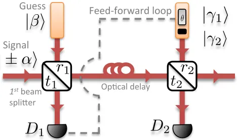
Figure 2. Schematic of the state comparison amplifier with state correction. Bob attempts to achieve destructive inter-ference in both the output arms which are fed into the detectors. This time, if the first detector fires, he can still correct the output by suitably changing the input state of the second comparison stage via the amplitude and phase modulator (in this case the outcome of the second detector is disregarded).

2. SCAMP WITH FEED-FORWARD STATE CORRECTION

Let us now consider a new system comprising of two comparison stages as shown in figure2. Again, Alice will choose a state uniformly at random while Bob this time has to choose two input states, one for each comparison beam splitter.

The first comparison stage is operated as before. If the first detector does not fire Bob has no reason to believe his initial guess was wrong and will continue the amplification process by mixing the output of the first comparison stage accordingly (i.e., with the state|β2i=|_rt₁2_r2αi if he has chosen|_rt1₁αiat the previous stage) and if also the second detector does not fire he takes this as an imperfect indication that his guess was right and that the output contains the correct amplified state. If Alice’s choice was|+αithe output state is given by | α

r1r2i, henceforth the gain of the device is given by g

2 ₌ 1

r2

1r22. The device output given both the comparison

detectors did not fired is given by:

ρout|71,72 =p

α r1r2

ED α

r1r2

+ (1−p)

2r2 1r22−1

r1r2

αED2r

2 1r22−1

r1r2

α

with p=

P(71,72|+α)

P(71,72)

P(+α). (5)

On the other hand, if the second detector does fire Bob knows for sure that his guess was wrong in first place and simply discards the output. Note that again the probability for both the detectors to not fire is maximised when Bob’s guess is right.

Suppose now the first detector does fire, then Bob knows that his guess was wrong but he can still correct the final output if the device allows him to choose the appropriate correcting input state for the second comparison stage. More precisely, suppose Bob’s first input was_|β1i=|tr11αi, if the first detector fires, Bob can correct the

output by inserting in the second beam splitter the state_|γ2i= 1

t2

_−1−r2 2(t

2 1−r

2 1)

r1r2

αE. In this case there is in principle no need to monitor the second detector counts as Bob knows he is correct.

The success scenarios of the device can be summarised in the following table, where the events corresponding to successful post-selection are highlighted in green:

SCAMP Success Scenario

D1 D2 Bob’s input 1st BS Bob’s input 2ndBS Output

7 7 |t1

r1αi |

t2

r1r2αi ρout|71,72

7 3 |t1

r1αi |

t2

r1r2αi A

3 7 |t1

r1αi |

1

t2

_−1−r2 2(t21−r21)

r1r2

α_{i |r}−α

1r2i

3 3 |t1

r1αi |

1

t2

_−1−r2 2(t

2 1−r

2 1)

r1r2

Summing up, provided that the correction strategy can be enacted, the successful events are given by the following set of detection outcomes:

S =

{D1=7, D2=7}, D1=3 . (6)

Note that the amplitude of the states_|β2iand|γ2ihave opposite phases and the second is larger in magnitude†. The benefit of the state correction strategy is now apparent, it increases both the success probability and the fidelity, compared to the single comparison stage, by including in the success scenarios an event that corresponds to exact amplification.

3. PERFORMANCE ANALYSIS

Bearing in mind the mechanism by which Bob has to choose the input states at the second stage, we can now compute the success probability for the new device. For sake of simplicity sake we will assume that the two comparison beamsplitters identical, i.e. r1=r2=r, and detection efficiency η1=η2=η:

P(S) =P(72,71) +P(72,31) +P(32,31) (7)

=P(72,71) +P(31) (8)

= X

σ={+α,−α}

(P(72,71|β2, β1, σ) +P(31|β1, σ))P(σ) (9)

=1 2

1 +e−4η

1−1

g2 α2 +1 2

1₋e−4η(1−1g)α

2

. (10)

Since there is no knowledge about the input state we have thatP(+α) =P(−α) = 1₂. Furthermore we have that

P(72,71|β2, β1,+α) = 1 andP(31|β1,+α) = 0 and the rest of the probabilities are computed in appendixA. Let us now consider the success probability-fidelity product and as before we assume that Bob’s initial guess was_|β1i=|rt11αi:

P(T, S) =P(T,72,71) +P(T,31) (11)

= X

σ={+α,−α}

(P(T,72,71|β2, β1, σ) +P(T,31|γ2, β1, σ))P(σ) (12)

= X

σ={+α,−α}

P(T|72,71, β2, β1, σ) +P(T|31, γ2, β1, σ)P(31|β1, σ)P(σ). (13)

The probabilities of passing the measurement test for a given set of input and guess state can be readily computed as:

P(T_|72,71, β2, β1,+α) =|hgα|gαi|2= 1, (14)

P(T_|72,71, β2, β1,−α) =|hg 1−2/g2α| −gαi|2, (15)

P(T_|31, γ2, β1,+α) = 0, (16)

P(T_|31, γ2β1,−α) = 1, (17)

whereP(T|31, γ2, β1,+α) = 0 is understood as the detector cannot trigger due to a correct guess. The overlap of two coherent states, say|σ1iand|σ2iis:

|hσ1|σ2i|2=e−|σ1−σ2|

2

. (18)

The success probability-fidelity product is thus given by:

P(T, S) =1 2

1 +P(72,71|β2, β1,−α)|hg 1−2/g2α| −gαi|2+P(31|γ2, β1,−α)

(19)

=1 2

1 +e−4η

1−1

g2

|α|2

e−4g2

1−1

g2

2

|α|2

+ 1−e−4η(1−g1)|α|

2

. (20)

†

It is easy to see that γ2

β2 = 2t

2 1

_t2 2−1

t2 2

−1<0 and that

γ2 β2

−1 = 2t

2 1

_1−t2 2

t2 2

0.0 0.2 0.4 0.6 0.8 1.0 1.2 1.4

|

α

2

0.6 0.7 0.8 0.9 1.0

P

(

T

|

S

)

0.0 0.2 0.4 0.6 0.8 1.0 1.2 1.4 |α

2

0.6 0.7 0.8 0.9 1.0

P(T|S)

g2_{=5,η=1, SCAMP+FF}

g2_{=8,η=1, SCAMP+FF}

g2_{=11,η=1, SCAMP+FF}

g2_{=5,η=0.4, SCAMP+FF}

g2_{=8,η=0.4, SCAMP+FF}

g2_{=11,η=0.4, SCAMP+FF}

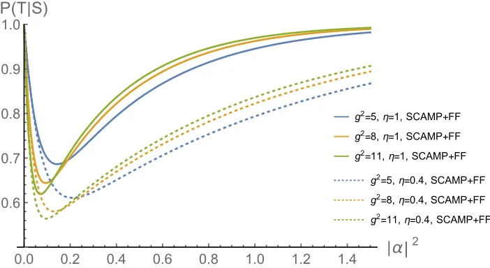
Figure 3. Success probability-fidelity product as a function of the input mean photon number for various values of the gaing2 for the SCAMP with feedforward state correction. Solid lines (dashed) correspond to a detection efficiency of 1 (0.4).

The success probability-fidelity product is plotted in figure3. All the curves show a similar pattern: P(T, S) at first decreases until it reaches a minimum, whose position depends on the gain and the detection efficiency, after that it increases until it asymptotically reaches one.

This trend is due to the fact that for low input mean photon number it is very unlikely for the detectors to trigger even when the guess is wrong, this causesP(T, S) to decrease until the probability for the first detector to trigger become significant, thus enacting state correction. As can be appreciated, this turning point is reached for lower mean photon number as the gain increases but it corresponds to a deeper minimum. The effect in the success probability-fidelity product of inefficient detection does not change this behaviour but it pushes the recovery to higher mean photon number as it decreases the probability of registering events at the detectors.

4. COMPARISON WITH UNAMBIGUOUS STATE DISCRIMINATION (USD)

The problem of amplifying an unknown coherent state can be recast as the problem of discriminating between the coherent states in the set and subsequently outputing an amplified version of that state. The optimal probability with which a symmetric set of coherent states, a priori equiprobable and with known mean photon number, can be unambiguously discriminated has been computed in5_{for an arbitrary state space dimension. For a two state}

space, the best possible success probability is given by:

PU SDopt = 1−e −2|α|2

. (21)

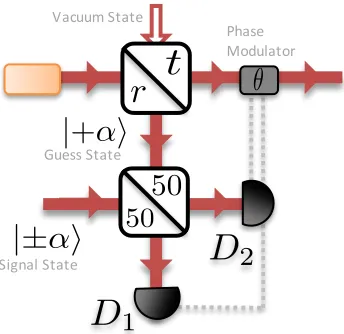
Remarkably, the bound can be achieved by using equivalent experimental means to SCAMP, an experimental realisation of it is sketched in figure,?_{note that feed-forward capability is also needed in this case. The unknown}

quantum state is mixed at a 50:50 beam splitter with (say) the state_|+α_i, depending on the input state, all the light will go in one of the two output arms while the other will be in the vacuum state. Hence a detector triggering will provide an unambiguous indication of what the input state was, while no detector firing will leave Bob no wiser. The phase modulator imprint the correct phase on the output based on the detection outcomes, the device’s gain is given byg2₌ t2

r2. Taking into account detection inefficiency the previous expression reads:

PU SD= 1−e−2η|α|

2

. (22)

50

50

|±

r

t

Phase& Modulator

D

1

D

2

|

+

Guess&State

Signal&State Vacuum&State

Figure 4. Schematics for the optimal USD-based amplifier for two states.

0.0 0.2 0.4 0.6 0.8 1.0 1.2 1.4 |α

2

0.6 0.7 0.8 0.9 1.0

P(T)USD

g2_{=5,η=0.4, USD+CF}

g2_{=8,η=0.4, USD+CF}

g2_{=11,η=0.4, USD+CF}

g2_{=5,η=0.4, USD+CF}

g2_{=8,η=0.4, USD+CF}

g2_{=11,η=0.4, USD+CF}

0.0 0.2 0.4 0.6 0.8 1.0 1.2 1.4

|

α

2

0.6 0.7 0.8 0.9 1.0

P

(

T

)

g

₌

_5,

_η

₌

_{0.4, USD}

₊

_CF

g

=

8,

η

=

0.4, USD

+

CF

g

=

11,

η

=

0.4, USD

+

CF

g

=

5,

η

=

0.4, USD

+

CF

g

=

8,

η

=

0.4, USD

+

CF

g

=

11,

η

=

0.4, USD

+

CF

Figure 5. Success probability-fidelity product as a function of the input mean photon number for various values of the gaing2for the USD plus coin-flip. Solid lines (dashed) correspond to a detection efficiency of 1 (0.4).

It is natural to compare a USD based system with the SCAMP. Being unambiguous, the fidelity of a USD based system is always equal to one, at least in an ideal case that does not take into account unavoidable experimental imperfections such as dark counts and interferometer misalignment.

Here we compare the success probability-fidelity product. In order to carry out a fair comparison we have also considered a case when the USD based system is allowed, when inconclusive, to randomly flip a coin and output an amplified state, note that when no detector registers an event this is the best strategy as Bob has not gained any information about the input state, in this case the success probability is unity and the probability of passing a measurement test with the amplified output is given by:

P(T)U SD=PU SD+ (1−PU SD)

1 2

1 +e−4g2|α|2. (23)

0.2 0.4 0.6 0.8 1.0 1.2 1.4

|

α

4 6 8 10

Δ

[%]

g2_=5,η=0.4

g2_=8,η=0.4

g2_=11,η=0.4

0.2

0.4

0.6

0.8

1.0

1.2

1.4

|

α

2

2

4

6

8

10

Δ

[%]

Figure 6. Percentage advantage of the feed-forward SCAMP with respect to the USD plus coin-flip as a function of the input mean photon number for various values of the gaing2_.

in this case, the effect in the success probability-fidelity product of inefficient detection does not change this behaviour but it pushes the recovery to higher mean photon number as it decreases the probability of registering events at the detectors.

In figure 6it is plotted the percentage advantage of the SCAMP with feedforward with respect to the USD plus coin-flip, i.e.:

∆ = 100P(T, S)−P(T)U SD

P(T)U SD

. (24)

In this plot we considered a detection efficient of 0.4 in order to present a real case scenario. The success probability-fidelity product of the SCAMP with feedforward state correction is always higher (up to 10%) than the one of the USD plus random output when inconclusive. The advantage is at least 2% for all the mean photon number considered.

5. CONCLUSIONS

We presented an high rate, high gain approximate probability amplifier with state correction based on feed-forward. The success probability-fidelity product of this device is always higher than the on of the USD plus random output when inconclusive.

This system can be realised with classical resources (i.e., lasers, linear optics and APD detectors). Similar systems, with no state correction, proved to achieve high-gain, high fidelity and high repetition rates16,17and.18 The ability to switch between input states on the fly requires delay lines and fast switching but it can still achieved with classical resources.

Due to its simplicity, the system we propose might represent an ideal candidate as a recovery station to counteract quantum signal degradation due to propagation in a lossy fibre or as a quantum receiver. The system is also suitable for on-chip implementation.

APPENDIX A. AMPLITUDE CALCULATION

Here we compute the coherent amplitudes reaching the detectors in the outputs of the first and the second comparison beam splitters. If Bob’s guess is right, i.e. Alice has chosen _|+α_i, we have that:

t1 r1 −r1 t1

t1

r1α

α

=

α

r1

0

On the other hand if Bob’s guess was wrong, i.e. Alice has chosen|−αi, we have that:

t1 r1 −r1 t1

t1

r1α

−α

=

"

t2₁−r2 1

r1 α

−2t1α #

. (26)

We can use the Kelly-Kleiner formula19 _{to compute the probability of a detection outcome. Assuming a}

detection efficiency ofη1, we have that the probability of recording or not one event are respectively given by:

P(71|β1,+α) = e−η1|0|

2

= 1, (27)

P(71|β1,−α) = e−η1|2t1α|

2

, (28)

P(31|β1,+α) = 1−e−η1|0|

2

= 0, (29)

P(31|β1,−α) = 1−e−η1|2t1α|

2

. (30)

Let us now consider the second comparison beam splitter. If Bob’s guess is right, we have that:

t2 r2 −r2 t2

t2

r2r1α

α r1

=

α

r2r1

0

. (31)

If Bob’s guess is wrong and the first detector did not fired, we have that:

t2 r2 −r2 t2

" t2

r2r1α

t2₁−r2 1

r1 α

# =

" 1−2r2

1r22

r1r2 α

−2t2r1α #

. (32)

On the other hand, if the first detector fires Bob can correct the out by using as second input the state

1

t2

_−1−r2 2(t

2 1−r

2 1)

r1r2

αE, in fact we have that:

t2 r2 −r2 t2



 1

t2

_−1−r2 2(t21−r21)

r1r2

α

t2 1−r21

r1 α



=

− α r1r2

. . .

. (33)

Note that in this case the output of the second beam splitter is simply disregarded. We can thus compute the probability of the remaining events:

P(72,71|β2, β1,+α) = e−η1|0|

2

e−η2|0|2_{= 1, (34)}

P(72,71|β2, β1,−α) = e−η1|2t1α|

2

e−η2|2r1t2α|2_{. (35)}

ACKNOWLEDGMENTS

The work was supported by the UK Quantum Technology Hub for Quantum Communications Technologies funded by UK Engineering and Physical Sciences Research Council (EP/M013472/1).

REFERENCES

[1] Caves, C. M., “Quantum limits on noise in linear amplifiers,”Phys. Rev. D26, 1817–1839 (Oct 1982). [2] Ralph, T. C. and Lund, A. P., “Nondeterministic noiseless linear amplification of quantum systems,”AIP

Conference Proceedings1110(1), 155–160 (2009).

[3] Pandey, S., Jiang, Z., Combes, J., and Caves, C. M., “Quantum limits on probabilistic amplifiers,” Phys. Rev. A88, 033852 (Sep 2013).

[4] Eleftheriadou, E., Barnett, S. M., and Jeffers, J., “Quantum optical state comparison amplifier,”Phys. Rev. Lett.111, 213601 (Nov 2013).

[6] Bennet, C. H. and Brassard, G., “Quantum cryptography: Public key distribution and coin tossing,”Proc. of IEEE Int. Conf. on Comp., Syst. and Signal Proc., Bangalore, India, Dec. 10-12, 1984, 175–179 (1984). [7] Gisin, N., Ribordy, G., Tittel, W., and Zbinden, H., “Quantum cryptography,”Rev. Mod. Phys.74, 145–195

(Mar 2002).

[8] Campagna, M. and et al., [Quantum Safe Cryptography and Security], vol. 8, ETSI, 979-10-92620-03-0 (June 2015).

[9] Mazzarella, L., Ticozzi, F., Sergienko, A. V., Vallone, G., and Villoresi, P., “Asymmetric architecture for heralded single-photon sources,”Phys. Rev. A88, 023848 (Aug 2013).

[10] Branny, A., Kumar, S., Proux, R., and Gerardot, B., “Deterministic strain-induced arrays of quantum emitters in a two-dimensional semiconductor,”Nature Communications8, 15053 EP – (May 2017). [11] Sasaki, M., Fujiwara, M., Ishizuka, H., Klaus, W., Wakui, K., Takeoka, M., Miki, S., Yamashita, T., Wang,

Z., Tanaka, A., Yoshino, K., Nambu, Y., Takahashi, S., Tajima, A., Tomita, A., Domeki, T., Hasegawa, T., Sakai, Y., Kobayashi, H., Asai, T., Shimizu, K., Tokura, T., Tsurumaru, T., Matsui, M., Honjo, T., Tamaki, K., Takesue, H., Tokura, Y., Dynes, J. F., Dixon, A. R., Sharpe, A. W., Yuan, Z. L., Shields, A. J., Uchikoga, S., Legr´e, M., Robyr, S., Trinkler, P., Monat, L., Page, J.-B., Ribordy, G., Poppe, A., Allacher, A., Maurhart, O., L¨anger, T., Peev, M., and Zeilinger, A., “Field test of quantum key distribution in the tokyo qkd network,”Opt. Express19, 10387–10409 (May 2011).

[12] Clarke, P., Collins, R., Dunjko, V., Andersson, E., Jeffers, J., and Buller, G., “Experimental demonstration of quantum digital signatures using phase-encoded coherent states of light,” Nature Communications 3, 1174 EP – (Nov 2012).

[13] Donaldson, R. J., Collins, R. J., Kleczkowska, K., Amiri, R., Wallden, P., Dunjko, V., Jeffers, J., Andersson, E., and Buller, G. S., “Experimental demonstration of kilometer-range quantum digital signatures,” Phys. Rev. A93, 012329 (Jan 2016).

[14] Buller, G. S. and Collins, R. J., “Single-photon generation and detection,”Measurement Science and Tech-nology21(1), 012002 (2010).

[15] Van Enk, S. J., “Unambiguous state discrimination of coherent states with linear optics: Application to quantum cryptography,” Phys. Rev. A66, 042313 (Oct 2002).

[16] Usuga, M., M¨uller, C., Wittmann, C., Marek, P., Filip, R., Marquardt, C., Leuchs, G., and Andersen, U., “Noise-powered probabilistic concentration of phase information,”Nature Physics6, 767 EP – (Aug 2010). [17] Donaldson, R. J., Collins, R. J., Eleftheriadou, E., Barnett, S. M., Jeffers, J., and Buller, G. S., “Exper-imental implementation of a quantum optical state comparison amplifier,” Phys. Rev. Lett. 114, 120505 (Mar 2015).

[18] Donaldson, R. J., Mazzarella, L., Collins, R. J., Jeffers, J., and Buller, G. S., “A high gain, high fidelity and scalable quantum optical coherent state amplifier,”In preparation.