Study of the development of three-dimensional sets of fluid particles and iso-concentration fields using kinematic simulation

particles and iso-concentration fields using kinematic simulation

.

White Rose Research Online URL for this paper:

http://eprints.whiterose.ac.uk/1612/

Article:

Nicolleau, F.C.G.A. and Elmaihy, A. (2004) Study of the development of three-dimensional

sets of fluid particles and iso-concentration fields using kinematic simulation. Journal of

Fluid Mechanics, 517. pp. 229-249. ISSN 0022-1120

https://doi.org/10.1017/S0022112004000898

[email protected] https://eprints.whiterose.ac.uk/ Reuse

Unless indicated otherwise, fulltext items are protected by copyright with all rights reserved. The copyright exception in section 29 of the Copyright, Designs and Patents Act 1988 allows the making of a single copy solely for the purpose of non-commercial research or private study within the limits of fair dealing. The publisher or other rights-holder may allow further reproduction and re-use of this version - refer to the White Rose Research Online record for this item. Where records identify the publisher as the copyright holder, users can verify any specific terms of use on the publisher’s website.

Takedown

If you consider content in White Rose Research Online to be in breach of UK law, please notify us by

DOI: 10.1017/S0022112004000898 Printed in the United Kingdom

Study of the development of three-dimensional

sets of fluid particles and iso-concentration fields

using kinematic simulation

By F. C. G. A. N I C O L L E A UA N D A. E L M A I H Y

Department of Mechanical Engineering, University of Sheffield, Mapping Street, Sheffield S1 3JD, UK

(Received2 February 2003 and in revised form 24 June 2004)

We use kinematic simulation (KS) to study the development of a material line im-mersed in a three-dimensional turbulent flow. We generalize this study to a material surface, cube and sphere. We find that the fractal dimension of the surface can be explained by the same mechanism as that proposed by Villermaux & Gagne (Phys. Rev. Lett.vol. 73, 1994, p. 252) for the line. The fractal dimension of the line or the surface is a linear function of time up to times of the order of the smallest characteristic time of turbulence (or Kolmogorov timescale). For volume objects we describe the respective role of the Reynolds number and of the object’s characteristic size. Using the method of characteristics with KS we compute the evolution with time of a concentration fieldC(x_{, t) and measure the fractal dimension of the intersection of this}

scalar field with a given plane. For these objects, we retrieve the result of Villermaux & Innocenti (J. Fluid Mech. vol. 393, 1999, p. 123) that the Reynolds number does not affect the development of the fractal dimension of the iso-scalar surface and extend this result to volume geometries. We also find that for volume objects the characteristic time of development of the fractal dimension is the large scales’ characteristic time and not the Kolmogorov timescale.

1. Introduction

large-Reynolds-number computations or, more exactly, large ratios of inertial range scales, the very range where the fractal dimension is to develop.

The paper is organized as follows: this first section introduces the basics of kinematic simulation and particle tracking. Section 2 deals with the line,_§3 with the plane and

§4 with the volume. Section 5 complements_§4 with the study of an iso-scalar object. Finally,_§6 concludes this paper.

1.1. Kimematic simulation

Kinematic simulations (KS) are Lagrangian models of turbulent diffusion based on kinematically simulated turbulent velocity fields which are non-Markovian (not Dirac-correlated in time), incompressible and consistent with up to second-order statistics of the turbulence such as energy spectra. (See for instance Funget al.(1992) for more details on the assumptions underlying KS.)

Kinematic simulations can reproduce detailed statistics of the Lagrangian velocity field such as flatness factors of Lagrangian relative velocities (Malik & Vassilicos 1999). By comparison to a Wiener process which causes fluid element pairs to separate in Lagrangian models of relative diffusion based on Langevin-type equations, the mechanism by which fluid element pairs separate in KS might be comparable to that in turbulent flows.

In practice, the KS approach relies on the integration of dx

dt =u(x, t), (1.1)

where x _{is the position of the fluid particle and} u_{a turbulent-like Eulerian velocity}

field. Statistics are then performed on the trajectories. Incompressibility is enforced in the construction of u_{and the energy spectrum is prescribed according to the type of}

turbulence considered.

KS can be used to track particles with inertia (Fung, Hunt & Perkins 2003) and in some cases it can be extended to no isotropic turbulence (Nicolleau & Vassilicos 2000), but here we will only consider fluid particles released in a three-dimensional isotropic turbulence.

Ifu₍x_{, t) is known, solving (1.1) is straight forward; but solving}u₍x_{, t) at every point}

and time can be difficult. Because of the computational expense of DNS, kinematic simulations have been proposed to simulate Lagrangian properties of turbulent flow fields. In KS, random flow fields are generated whose statistics agree with values obtained from experimental measurements or other reliable numerical simulations. KS use an analytical formula for u₍x_{, t), therefore they are not grid-based and no}

interpolation of the velocity field is needed.

In this paper, we use a three-dimensional KS similar to that of Nicolleau & Yu (2004). The Eulerian velocity field used in (1.1) is generated as a sum of random Fourier modes. Incompressibility is enforced by construction of the velocity field in every realization. The energy spectrum is prescribed to take a₋5/3 power law form (see also Funget al. 1992; Elliott & Majda 1996; Fung & Vassilicos 1998; Malik & Vassilicos 1999; Nicolleau & Vassilicos 2003).

1.2. The velocity field

As in Nicolleau & Yu (2004), our three-dimensional KS velocity field is given as a sum ofN random Fourier modes, i.e.

u₍x_{, t) =}

N

n=1

k_{n defined as}k_n=k_n/|k_{n| is a random unit vector so that}

k_n=|k_n|k_n=|k_n|   

sinθncosφn

sinθnsinφn

cosθn  

, (1.3)

where θn∈[0,π] andφn∈[0,2π] are picked randomly in each mode and realization.

a_{n and} b_{n are random and uncorrelated vectors with their amplitudes being chosen}

according to a prescribed power law energy spectrumE(k), i.e.

|a_n|2_=|b_n|2₌ 2

3E(kn)kn (1.4)

and

E(k) = u

2 0

k1

k k1

−5/3

fork16k6kN,

E(k) = 0 otherwise.

    

(1.5)

Typical turbulence parameters we vary are the integral length scale

L= 3π 4

kN

k1

E(k)k−1dk

kN

k1

E(k) dk

(1.6)

in the limit of large Reynolds numbers (i.e.kN→ ∞)

L_≃ 3π

10 1

k1

= 3 20L1,

the turbulent velocity fluctuation intensity, defined by

u′=

2 3

E(k) dk

note that

u′_≃u0

for large enough Reynolds numbers and the Kolmogorov length scale, defined by

η= 2π

kN

.

Hence, in KS, rather than the Reynolds number, the natural parameter is the ratio

L1/η=kN/ k1 which is input data of the computation. An order of magnitude for the

Reynolds number (Re) can be obtained from the relation Re_∼ L

η

4/3

.

We will see later on how we can calibrate an equivalent Reynolds number for the KS. In this paper, the distribution of the wavenumber is geometric, i.e.

kn=k1

kN

k1

(n−1)/(N−1)

100 101 102 103 104

10–1 ₁₀0 ₁₀1

–lnǫ

102 L/3

3η

ln Nb

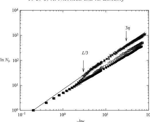
Figure 1.lnNb as a function of−lnǫ for different values ofλ. The box-counting was made

att= 0.057L/u′forL1/η= 178. Different curves corresponds to +,λ= 0;×,λ= 0.5;∗,λ= 1; 䊐_, λ_{= 5;} 䊏_, λ_{= 20. The line corresponds to the best fit curve between the two arrows, i.e.} y= 8.7x1.199_.

It is possible to introduce a frequencyωnthat determines the unsteadiness associated

with thenth wavemode. Malik & Vassilicos (1999) chose it to be proportional to the eddy-turnover time of thenth wavemode, i.e.

ωn=λ

k3

nE(k), (1.8)

whereλ _{is the unsteadiness parameter and may be expected to be of the order of 1.}

It has been shown in isotropic turbulence (Malik & Vassilicos 1999) that for two-particle diffusion a significant number of statistical properties are insensitive to the unsteadiness parameter value in the range 06λ61 in three-dimensional KS. In accordance with these results, we do not add any unsteadiness term to the KS. This is particularly justified here as we are not interested in the large-time random walk regime of the fluid particle diffusion. In this paper, particles are tracked for times smaller than 2/3 of the characteristic timeτd=u′/L. This result is further illustrated

in figure 1. As discussed in _§2, the fractal dimension is measured from the slope of the line fitting the points between the two arrows in figure 1. We repeat the results for

λ_{= 0, 0.5, 1, 5 and 20. As can be seen,}λ_{has no effect on these points provided that it}

is in the range [0,1]. Forλ_{>1, the fractal dimension tends rapidly to 1 as}λ_increases,

i.e. there is no turbulence structure. This is because the velocity field will be flapping so fast at all scales that the fluid elements do not have the time to experience the effect of eddying, streaming and straining flow structure (Malik & Vassilicos 1999).

It should also be noted from the constructed velocity field (1.2) that the coefficients of the nth Fourier mode are normal to k_{n ensuring the incompressibility of the}

velocity field trajectory by trajectory.

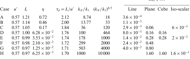
In table 1 we summarize the different cases we run varyingLandη. 1.3. Fractal dimension from kimematic simulation

0/ηfor

Case u′ L η τd=L/u′ kN/ k1 (kN/ k1)4/3 Line Plane Cube Iso-scalar

A 0.57 1.21 0.72 2.12 8.74 18 3.6_×10−4

B 0.57 1.14 0.46 2.00 13.77 33 1.1×10−3

C 0.57 1.05 0.17 1.84 36 120 2.9_×10−3 _{0.06 6×10}−3

D 0.57 1.00 6.28×10−2 _{1.76 100 464 8.0×10}−3 _{0.16 0.16}

E 0.57 0.99 3.53_×10−2 _{1.74 178 1000 1.4×10}−2 _{0.28 0.28 2×10}−2 F 0.57 0.98 2.10×10−2 _{1.72 299 2000 2.4×10}−2 _0.48

G 0.57 0.97 1.25_×10−2 _{1.71 503 4000 4.0×10}−2 _0.80

H 0.57 0.97 6.25×10−3 _{1.70 1000 10 000 1.60 1.60 1.6×10}−1

Table 1. Different KS case summary,0 is the initial distance separating two

neighbouring points.

Reynolds numbers. In this paper, we are more interested in the development of the fractal dimension of a line or surface than in its final value. As shown by Villermaux & Gagne (1994), this evolution is linked to the turbulence scales existing in the flow and this is a good validation for KS.

In practice, particles are released from their initial position at an initial timet0 that

for the sake of simplicity we set to 0, then we use KS to track the particle trajectories. The line discretization0is fixed att0, the corresponding values for0/ηare reported

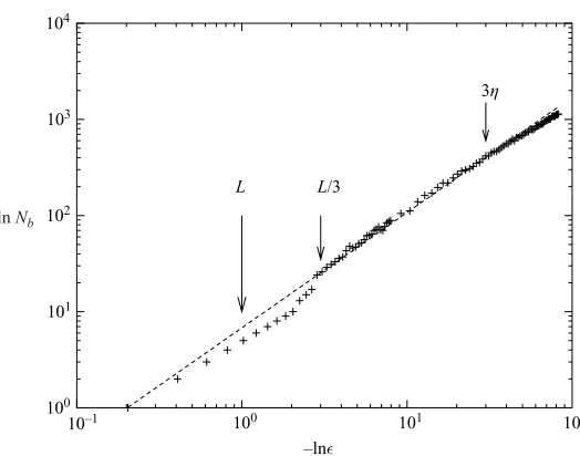
in table 1. This initial distance is chosen small enough so that it remains small during the diffusion process for the fractal dimension to be accurate. In the case of the line, the r.m.s value of the distance between two neighbour particles is always at least 10 times smaller than the Kolmogorov length scale when we stop the computation. For other geometries, we could not afford that precision for all Reynolds numbers, but this was maintained at least for Re<4000 and no particularities were observed in the two cases Re>4000. At any time we can measure the fractal dimension of the set of points formed by the points where the particles are. We use the modified box-counting method of Buczkowski et al. (1998) to compute the fractal dimension. A case is shown in figure 2 where we plot the number of boxes Nb as a function of

the inverse of the size of the box 1/ǫ. There is a fractal dimension ifNb is a power

law of ǫ, that is in a logarithmic plot:

lnNb=−Dlnǫ+C,

where D is the fractal dimension. Figure 2 is representative of our results, for all fractal dimensions that we measured we observed the power law over more than 1 decade or a minimum range of [L/3,3η].

1.4. Evolution of an iso-scalar field

We can also use kinematic simulation to predict the evolution of a blob of concen-tration released in a turbulent velocity field and compute its fractal dimension as a function of time.

100 101 102 103 104

10–1 100 ₁₀1

–lnǫ

102

L L/3

3η

ln Nb

Figure 2.Precision of the box-counting method used in the computation of the fractal dimension. lnNbas a function of−lnǫatt= 0.057L/u′forL1/η= 178.

2. Fractal dimension of an initially one-dimensional line

The development of a fractal line was studied in (Nicolleau 1996); numerical re-sults from a large eddy simulation were compared to experiments and theory from Villermaux & Gagne (1994). A general formula was proposed for the fractal dimension of the lineDl:

Dl−1

0.088Re1/2 =

t τd

, (2.1)

whereτd=L/u′ is the turnover time. However, this was only validated for a limited

range of Reynolds numbers and the numerical method then used was an LES which by construction does not resolve small-scale turbulence.

However, two-particle statistics are very significantly influenced by the entire range of flow structures (see e.g. Batchelor 1952). So, it is important to validate (2.1) with large Reynolds numerical experiments that involve large ratios of length scales and KS can do that.

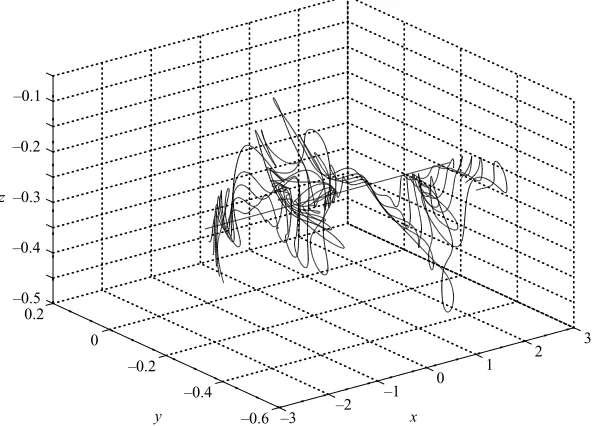
Initially, the particles are released in the horizontal planez=₋0.25Lon a line from point (₋2.5L, 0.25L) to point (2.5L, 0.25L) as shown in figure 3. The parameters of the different turbulences considered are reported in table 1.

In figure 4, we plot (Dl−1)/0.088Re0.5 as a function oft /τd for experimental, LES

and KS results. KS results in figure 4 correspond to the cases A, B, C, D, E, F and G described in table 1. For experimental cases, we use for the Reynolds numbers the values provided in Villermaux & Gagne (1994). For KS, we define the Reynolds number as

Re= 30.25 L

η

4/3

= 2.61 L1

η

4/3

–3 –2

–1 0

1 2

3

–0.6 –0.4 –0.2 0 0.2 –0.5 –0.4 –0.3 –0.2 –0.1

x y

z

Figure 3. Evolution of a line embedded in turbulence as a function of time.

0 0.1 0.2

(D

l

– 1)/0.088

Re

1/2

0.3 0.4 0.5

0.1 0.2 0.3

tu′/L

0.4 0.5 0.6

Figure 4. Evolution of the normalized fractal co-dimension of a line (Dl−1)/0.088Re1/2 as

a function oft(u′/L): KS for (L1/η)4/3= 18 (+), 33 (×), 120 (∗), 464 (䊐), 1000 (䊏), 2000 (䊊)

and 4000 (䊉_{); Villermaux’s experimentRe= 18 (}M) and 33 (N); LES forRe= 120 (O).

This is because in the demonstration for (2.1), what matters is the range of scales over which the fractal process occurs. This range is the range over which the spectral₋5/3 power law is observed, that is [L1, η] in the case of KS. Whereas for experimental

spectra, the power law k−5/3 _{is observed over a range shorter than [L, η]. So for the}

10–2 10–1 100

102 103 ₁₀4 ₁₀5 1.0

1.1 1.2 1.3 1.4

0 1000 2000 3000 4000

τ_ms

τd

1 – 2

τ_ml

τ_d

(a) (b)

(L1/η)4/3 (L1/η)4/3

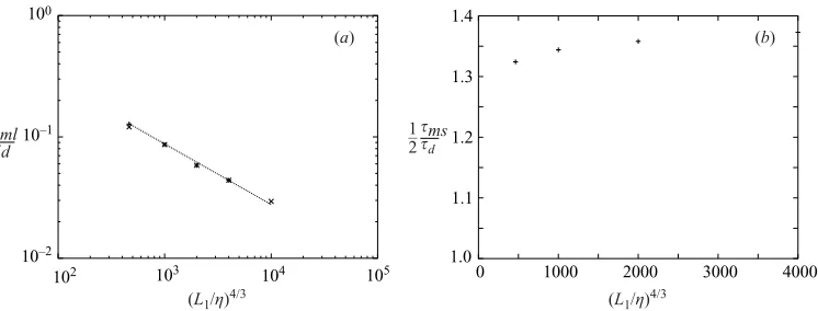
Figure 5.(a) +, non-dimensional time τml/τd at which the maximum fractal dimension of

the line is obtained as a function of (L1/η)4/3;×, re-scaled non-dimensional time (τms/τd)/2 at

which the maximum fractal dimension of the square is obtained as a function of (L1/η)4/3

(see§3.2). Interpolating line is τml/τd= 2.77(L1/η)−2/3. (b) Maximum fractal dimensionDmax reached by the line as a function of (L1/η)4/3.

from Villermaux & Gagne (1994). From now on, Reynolds numbers associated to a KS will use definition (2.2).

We observe that:

(i) The line’s fractal dimension obeys (2.1) withRe given by (2.2). It even catches the theoretical curve at small times better than the lines computed with LES. This is because the turbulence structures acting at small times have the smallest length scales and are the ones most likely to be influenced by the LES subgrid.

(ii) KS predicts an asymptotic valueDl≃1.37 (see figure 5b).

(iii) Equation (2.1) is still valid for large Reynolds numbers (up to L1/η= 503)

and figure 5bvalidates the fact that the time necessary to reach the asymptotic value

Dl≃1.37τml is proportional to 1/ √

Re. With KS we find

τml = 2.77

η L1

2/3

L

u′ = 0.81

_η

L

2/3 _L

u′ ≃τη. (2.3)

Having the line’s maximum dimension reached in such a short time may be surprising but, as a comparison, if we put the obvious upper bound Dl= 3 in (2.1) then we

obtain:

t(Dl = 3) = 22.7τη.

Hence, from the multiplicative approach adopted in Villermaux & Gagne (1994), the maximum fractal dimension has to be reached by few Kolmogorov time scales. Though there is no way to know this value from this theory. Earlier works by Meneveau & Sreenivasan (1990) (Sreenivasan, Ramshankar & Meneveau 1989) propose 1.336Dl6

1.36. Another approach by Queiros-Conde (1999, 2000) using the concept of entropic skins leads to the same order of magnitude forτml.

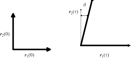
r2(0)

r1(0) r1(τ)

r2(τ)

θ

Figure 6. Shear and strain of an elementary square.

3. Fractal dimension of an initially two-dimensional surface

3.1. Theoretical analysis

Equation (2.1) was derived for a line using one-dimensional arguments. It was mainly derived from covering the line with segments and using the relation:

ǫ_≃ δu(r)

3

r , (3.1)

where ǫ is the turbulence dissipation rate, δu(r) the average velocity difference over a structure of size r (see e.g. Mathieu & Scott 2000, for the derivation of (3.1)). To generalize this result we investigate the fractal dimension of a two-dimensional object. Particles are released at t= 0 from an horizontal plane at z=₋0.1L on a square of size L see figure 7. The Villermaux & Gagne (1994) demonstration can easily be generalized to a plan. The difference in velocity at two points separated by a distance

r is written as

δu(r) =f r η

(ǫr)1/3

, (3.2)

with

f r η

→1 if r

η ≫1, f r

η

→ r_η

2/3

if r

η <1.

        

(3.3)

A convenient form is

f r η

= 1₋exp₋(r/η)2/3_{. (3.4)}

If we consider the initial plan square of area A0, it can be covered with elementary

squares of area a0=|r1×r2|. After a small interval of timeτ each elementary square

becomes distorted (figure 6) and the area of the distorted element is now

a(τ) =_|r_1(τ)×r_{2(τ)|=r1(τ)r2(τ) cosθ(τ) =r1(τ)r2(τ)}

1₋1 2

dr2

dr1

1

r2

τ

2

, (3.5)

that is at first order inτ

or as_|r_2(0)|=|r_1(0)|=r0=a1/2 0

a(τ)_≃a0+

∂u1

∂x1

(0)r02+

∂u2

∂x2

(0)r02

τ =a0

1 + ∂u1

∂x1

(0) +∂u2

∂x2 (0) τ . (3.7) This is where the plane development differs from the lines. Here we have to take into account the continuity equation

∂u1

∂x1

+ ∂u2

∂x2

+∂u3

∂x3

= 0. (3.8)

The stretchings along r1 and r2 have to be accounted together. Apart from that

constraint, if we set

α= ∂u1

∂x1

(0) +∂u2

∂x2

(0) =β1 r0

δu0, (3.9)

we can generalize the approach used in Villermaux & Gagne (1994) for a line to the plane: equation (3.7) becomes

a(τ)_≃a0+βδu0r0τ. (3.10)

The total area of the square is then

A(τ) =N0a(τ) =N0(a0+βδu0r0τ),

whereN0 is the initial number of elementary squares of area a0 needed to cover the

square at initial timet= 0. That is if we use equation (3.2),

A(τ) =N0 a0+βf

r0

η

ǫ1/3r₀4/3τ

. (3.11)

If we do the covering at timeτ, we will need

Nτ(a0) =

A(τ)

a0

=N0 1 +βf

r0

η

ǫ1/3r₀−2/3τ

of such elementary squares. For an interval of timet, this mechanism is reproduced

t /τ times so that:

Nt(a0) =N0 1 +βf

r0

η

ǫ1/3_r−2/3

0 τ

t /τ

. (3.12)

The dimension of the object is defined as

Ds(t) =−

d ln(Nt(a0))

d ln(r0)

r0=η

(3.13) withτ=τη. Using (3.4) we have:

Ds = 2 +

2 3

β

1 +β

e₋2 e₋1

t τη

, (3.14)

or using the relationτη= (L/u′)(η/L)2/3

Ds= 2 +

2 3

β

1 +β

1₋2/e 1₋1/e

L η

2/3

tL

u′. (3.15)

The plane deformation is a three-dimensional process constrained by the continuity equation, but we can try to set some boundaries for the value ofβ. According to (3.8), there is at least one positive and one negative value for∂ui/∂xi. Betchov (1956) has

shown that, on average, there are two positive values and one negative. Though in each particular realization of the velocity field there can be two negative values, such a situation would lead to the formation of an elongated one-dimensional structure and a smaller area and fractal dimension. We can first discard these cases and use the average picture where there are two positive and one negative values for ∂ui/∂xi,

this will provide an upper bound forβ and the fractal dimension. Let us set

∂u3

∂x3

< ∂u2 ∂x2

< ∂u1 ∂x1

. (3.16)

There are three possible configurations:

(i) All the stretching effects on the surface are positive i.e. the surface is subjected to

αi =

∂u1

∂x1

+ ∂u2

∂x2

. (3.17)

(ii) There is one negative stretching effect and the second one is the larger of the positive stretching effects:

αii=

∂u1

∂x1

+ ∂u3

∂x3

. (3.18)

(iii) The second one is the smaller of the positive stretching effects:

αiii=

∂u2

∂x2

+ ∂u3

∂x3

. (3.19)

In addition to the continuity equation, we also have the relation

δu2₀ r₀2 =

∂u1

∂x1 2

+ ∂u2

∂x2 2

+ ∂u3

∂x3 2

. (3.20)

In case (i) (3.20) can be re-written as

δu2₀ r₀2 =

∂u1

∂x1 2

+ ∂u2

∂x2 2

+ ∂u1

∂x1

+ ∂u2

∂x2 2

, (3.21)

that is

δu2₀ r2

0

= 2α_i2₋2∂u1

∂x1

∂u2

∂x2

or

αi2=

1 2

δu2 0

r₀2 + ∂u1

∂x1

∂u2

∂x2

.

Furthermore, in case (i) we have

06 ∂u2

∂x2 6 ∂u1

∂x1

,

so that

06 ∂u2

∂x2

∂u1

∂x1

6 ∂u1

∂x1 2

the upper bound is found for ∂u2/∂x2=∂u1/∂x1 and, in this case, a combination of

(3.8) and (3.20) yields

∂u1

∂x1 2

= 1 6

δu2₀ r2 0 . (3.22) So that 1 √ 2 δu0 r0

6αi 6

2 3 δu0 r0 . (3.23)

Similarly, in case (ii) (3.20) can be re-written as

δu2₀ r2

0

= ∂u1

∂x1 2

+ ∂u3

∂x3 2

+ ∂u1

∂x1

+∂u3

∂x3 2 , (3.24) that is δu2 0

r₀2 = 2α

2 ii−2

∂u1

∂x1

∂u3

∂x3

or

α_ii2 = 1 2

δu2 0

r₀2 + ∂u1

∂x1

∂u3

∂x3

. (3.25)

Furthermore, in case (ii) we have

∂u1 ∂x1 2 6 ∂u1 ∂x1 ∂u3 ∂x3 6 ∂u3 ∂x3 2 ,

the upper bound is found for ∂u1/∂x1=−∂u3/∂x3 and ∂u2/∂x2= 0 so that in this

case ∂u3 ∂x3 2 = 1 2

δu02

r₀2 .

The lower bound is found for∂u1/∂x1 minimum, that is ∂u1/∂x1=∂u2/∂x2, and we

can use (3.22). Asαii and (∂u1/∂x1)(∂u3/∂x3) are negative, (3.25) leads to −√1

6

δu0

r0

6αii 60. (3.26)

Case (iii) is similar to (ii) and we can deduce

α2_iii= 1 2

δu2₀ r2

0

+ ∂u2

∂x2 ∂u3 ∂x3 (3.27) and 06 ∂u2 ∂x2 ∂u3 ∂x3 6 ∂u1 ∂x1 ∂u3 ∂x3 ,

but now the upper bound is found for∂u2/∂x2 maximum, that is∂u2/∂x2=∂u1/∂x1,

in this case, we have already seen in (3.22) that (∂u2/∂x2)2= (δu20/r02)/6 so that

∂u3 ∂x3 2 = 2 3 δu2 0

r₀2 .

Asαiii and (∂u1/∂x1)(∂u3/∂x3) are negative, (3.27) leads to −√1

2

δu0

r0

6αiii6−

–1.0 –0.5

0

0.5 1.0

–1.0 –0.5 0 0.5 1.0 –1.0 –0.5 0 0.5 1.0

y z

x

Figure 7. Evolution of a set of particles released from an horizontal square in the plane z=₋0.1L, turbulence case E at timet= 0.09L/u′.

If all the three cases (i), (ii) and (iii) were as likely to occur, then an average value for α would be

α= 1

3(αi+αii+αii),

and then, using previous results, we can give an upper and lower bound for α

− 1

3√6

δu0

r0

6α6 1

3√6

δu0

r0

, (3.29)

that is in terms of K defined as follows:

Ds = 2 +K0.088

L η

2/3

tL

u′−0.236K60.23. (3.30)

However, this picture is unlikely, Batchelor (1952) and Girimaji & Pope (1990) showed that elementary surfaces align with the directions of maximum strain, hence case (i) is much more likely to occur than cases (ii) or (iii). We obtain an upper bound of all the possibilities when only (i) is present, which leads to

0.83< K <0.90. (3.31) So even in the best case for area increase, the increase is smaller than for the lines by at least 10%. From our KS results we findK_≃0.5, indicating something in-between the two extreme cases total isotropic distribution of the elementary squares (3.30) or total alignment (3.31).

3.2. KS analysis of a plane

We use KS to compute the fractal dimension of a set of particles released on a square at t= 0. The initial square is in the plane z=₋0.1L centred on (0,0,0) and has a side length of L. Each particle from the square is tracked so that we can follow the evolution of the square as a function of time. Figure 7 shows this evolution at

t= 0.15τd for the case referred to as E in table 1.

0.1 0.2 0.3

0 0.1 0.2 0.3

2(

D2

– 2)/0.088

Re

1/2

tu′/L

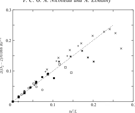
Figure 8.Evolution of the normalized fractal co-dimension 2(D2−2)/0.088Re1/2 of an

initially plane square as a function of t u′/L. Different ratios are: +, L1/η= 36; ×, 100; ∗, 178;䊐_{, 299;}䊏_{, 503;}⊙_{, 1000.}

2(D2−2)/0.088Re1/2 as a function of the non-dimensional time t u′/L varying the

Reynolds numbers. All the curves collapse, indicating a universal law similar to (2.1): (i) The surface fractal dimension of an initial plane obeys (3.32)

Ds−2

0.088Re1/2 =

1 2

t τd

, (3.32)

whereReis still defined by (2.2), that is

Ds = 2 + 0.044Re1/2t

u′

L (3.33)

or

Ds = 2 + 0.071

L1

η

2/3

tu

′

L.

This is verified for Reynolds numbers up toL1/η= 1000.

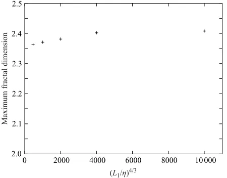
(ii) KS predicts the asymptotic valueDs≃2.4 (figure 9).

(iii) In figure 5, we plot τms/2 as a function of (L1/η)4/3, where τms is the time

necessary to reach the maximum fractal dimension for the square Ds≃2.4. We

observe that

τml= 1₂τms. (3.34)

(iv) As in the case of the line, we can see that the surface resolution decreases after

τms, resulting in a decrease of the surface dimension.

2.0 2.1 2.2 2.3 2.4 2.5

0 2000 4000 6000 8000 10 000

Maximum fractal dimension

(L1/η)4/3

Figure 9.Maximum fractal dimension reached by our KS for the square as a function of (L1/η)4/3.

We can deduce the formula for the area of the initial square as a function of time, by definition of the fractal dimension:

A(t)_≃L2s

Ls

η

Ds−2

=L2s

Ls

η

0.071(Ls/η)2/3_t(u′_/L)

, (3.35)

whereLs is the smaller ofL1 and the size of the square.

4. Fractal dimension of an initial volume object

Investigating a volume leads to a very different picture. The mechanisms leading to the line and surface development rely on the two positive eigenvalues of the velocity tensor (Girimaji & Pope 1990). Whereas in the case of the volume, we have to take into account the three eigenvalues of the velocity tensor and in the case of an incompressible flow, the total volume has to be conserved.

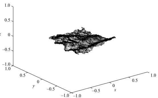
We released particles from cubes of different size s and a sphere of diameter

d= 0.2L, use KS to track the particles and then measure the fractal dimensionDv of

the set of particles as a function of time. For a three-dimensional object, there is both stretching and contraction and eventually the volume tends to contract to a sheet, as shown in figure 10.

We can apply our box-counting method to the cube to find the evolution of its fractal dimension as a function of time.

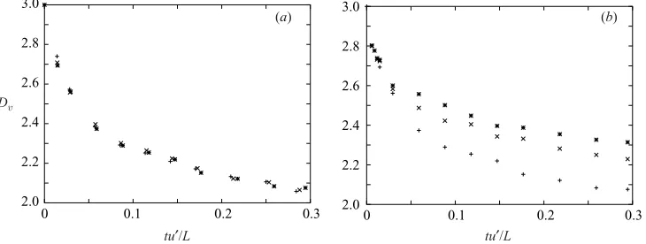
(i) Here, because of the contraction of the cube, the fractal dimension is decreas-ing. In figure 11, we plotDv the fractal dimension of what was initially a cube of size

s as a function of t u′/L for different ratios L1/η= 100, 178 and 1000 and different

cube sizess= 0.2L, 0.25Land 0.3L

–0.2 –0.1

0 0.1

–0.2 –0.1 0 0.1 0.2 –0.2 –0.1 0 0.1 0.2

x y

z

–0.2 –0.1

0 0.1 0.2

–0.2 –0.1 0 0.1 0.2 0.3 –0.2 –0.1 0 0.1

x y

z

(a) (b)

Figure 10. Evolution of a set of particles released from a cube in turbulence case E. (a) Initial cube, (b) particle cloud at timet= 0.17L/u′.

2.0 2.2 2.4 2.6 2.8 3.0

0 0.1 0.2 0.3 2.0

2.2 2.4 2.6 2.8 3.0

0 0.1 0.2 0.3

Dv

tu′/L tu′/L

(a) (b)

Figure 11.Evolution of the fractal dimension Dv of an initial cube as a function oft u′/L.

(a) For a given cube size s= 0.2L, the Reynolds number is varied; +,L1/η= 100; ×, 178; ∗, 1000. (b) For a given Reynolds number L1/η= 1000 the size of the cube is varied; +,

s= 0.2L;×,s= 0.25L;∗,s= 0.3L.

blob of concentration and concluded that the mixing time associated with the blob of concentration was independent of the Reynolds number, but a function of the size of the blob.

(iii) In figure 12, we plots(3₋Dv)/t u′as a function oft u′/Lfor different Reynolds

numbers and different ratioss/L. With this latter normalization, and using a logari-thmic plot, all the curves collapse onto a single line so that

s3−Dv

t u′ = 0.25

t u′ L

−2/3

. (4.1)

102

101

100

10–1

10–3 10–2 10–1 100

tu′/L

S

(3 –

Dv

)/

tu'

Figure 12. Re-scaled dimensions(3−Dv)/t u′ in logarithmic axes for all cases in figure 11.

L1/η= 1000: +, s= 0.2L;×, s= 0.25L;∗,s= 0.3L. s= 0.2L: 䊐,L1/η= 100; 䊏,L1/η= 178;

spherical source withd= 0.2LandL1/η= 1000. The fitting curve represented isy= 0.25x−2/3.

(iv) Equation (4.1) can be rearranged so that the fractal dimension of the initial cube Dv obeys

Dv = 3−

1 4

L s

t u′ L

1/3

. (4.2)

(v) The fractal dimension Dv is found to decrease towards 2 as t u′/L and L/s

increase.

5. Fractal dimension of an iso-scalar field

In practice, it is difficult to follow a three-dimensional object and most experi-mentalists look at iso-scalar surfaces (see, e.g. Lane-Serff 1993; Catrakis & Dimotakis 1996.) Villermaux & Innocenti (1999) made a detailed analysis of the evolution of the fractal dimension as a function of time.

Here, we study the evolution of a scalar whose initial concentration is

C(x, t) = 1 if_|x_|< d/2, C(x_{, t) = 0 otherwise.}

(5.1)

d is the source size. We use the method developed by Flohr & Vassilicos (2000) to obtain the points of the plane z= 0 such thatC(x_{, t) = 1, as shown in figure 13. The}

scalar diffusion is neglected so that the concentration field is governed by

∂C ∂t +uj

∂C ∂xj

= 0.

With no diffusion term, we can use the method of characteristics:C(x, t) is constant on a particle trajectory and we propose to use kinematic simulation (KS) to predict particle trajectories. At time t and point x _{we construct the particle’s trajectory}

–0.10 –0.05 0 0.05 0.10 0.15 –0.10

–0.05 0 0.05 0.10 0.15

x y

–0.2 –0.1 0 0.1 0.2 –0.2

–0.1 0 0.1 0.2

(a) (b)

Figure 13. Evolution of the region of concentrationc= 1 in the planez= 0 as a function of time. (a) Initial concentration, (b) concentrationc= 1 at timet= 0.17τd.

2.4 2.5 2.6 2.7 2.8 2.9 3.0

0 0.1 0.2 0.3 2.4

2.5 2.6 2.7 2.8 2.9 3.0

0 0.1 0.2 0.3

Di

tu′/L tu′/L

(a) (b)

Figure 14.Di as a function oft u′/L. (a) Different sources of a given sized= 0.15; spherical

source, (+)L1/η= 36, (×) 178, (∗) 1000 and cubical source, ( )L1/η= 1000. (b)L1/η= 1000,

sources of different sizes; (+)d= 0.15L, (×) 0.2L; (∗) 0.25L.

formula for the Eulerian velocity field, there is no problem in reversing the tracking method. Then, the concentration atx _{andt is the concentration that was att= 0 and} x_{(0) the particle initial position:}

C(x_{, t) =C(}x_{(0),0). (5.2)}

In practice, we compute the fractal dimension on a section that is the intersection of the fractal object with the planez= 0, then owing to isotropy, we assume that the fractal dimension of the fractal object embedded in the three-dimentional space is that of the section plus one. The advantage of this method is that while tracking the same number of points, we will obtain better resolution of the iso-scalar surface section. In figure 14 we show the fractal dimension as a function of the non-dimensional time

t u′/Lfor different Reynolds numbers Re, cases C, E and H in table 1.

In figure 15 we plot in a logarithmic graph the normalized co-dimensiond(3₋Di)/

t u′as a function oft u′/Lfor case H reported in table 1 and varying the ratiod/L. We observe a good collapse of the different cases on a line indicating thatd(3₋Di)/t u′

101

100

10–1

10–3 ₁₀–2 ₁₀–1 ₁₀0

102

d

(3 –

Di

)/

tu

′

tu′/L

Figure 15. Logarithmic plot of the evolution ofd(3−Di)/t u′as a function oft u′/L. Cubical

source,L1/η= 1000: +,s/L= 0.15;×,s/L= 0.20;∗,s/L= 0.25. Spherical source,L1/η= 1000: 䊐_{, d/L= 0.15;}䊏_{, d/L= 0.20;}⊙_{, d/L= 0.25. Spherical source, d/L= 0.15:} 䊉_{, L1/η= 36;} M, L1/η= 178. The trend line isy= 0.13x−2/3.

that is

Di = 3−0.13

t u′ L

1/3

L

d. (5.3)

This result has to be compared with (4.2) obtained for the cube. The two results are similar except for the coefficient 0.13 instead of 0.25. We should expect to find the same results when no diffusion is accounted for when considering the iso-scalar object. The discrepancy we find between the two coefficients is due to the method we use for computing the fractal dimension of the iso-scalar field. Tracking backward a complete three-dimensional field is too time consuming and we choose to consider only a section of the object, this may explain the ratio of 2 between the two coefficients. The assumption usually made that the dimension of the total object is that of a section plus one is not validated by our kinematic simulation.

It is worth commenting at this point on the form of (4.2) and (5.3) implying a different process from that involved in making the fractal dimension in lines and surfaces. As already mentioned, these equations are consistent with experimental results (Villermaux & Innocenti 1999) showing no dependence on the Reynolds number, but clear dependence on the source’s size. The dependence on the ratio L/s

is consistent with having L/u′ as the characteristic time for the dimension’s growth. Indeed, if we consider a box of size Laccording to (4.2), it will need a time L/u′ to reach its full fractal potential, that is, the maximum fractal co-dimension 3₋Dv over

the range of scales it contains, η to L. A portion d/L of this box will need a much smaller time as it must reach its fractal potential over a smaller range of scales.

6. Conclusion

fractal dimensions as functions of time. KS results for the line agree with previous experimental and numerical results. Dimensions of lines and planes vary linearly with time at least for times smaller than, or of the order of, the Kolmogorov timescaleτη.

The fractal dimension Ds of a material surface obeys a law similar to that found

for a material line:

Ds = 2 + 0.044

t τη

.

This is observed up to a time τms= 2τη and a maximum dimension Ds≃2.4. At any

timet < τml, the surface fractal co-dimension’s increase (Ds−2) is half that predicted

for the line. The characteristic time for the dimension’s growth is the Kolmogorov time micro-scaleτη.

The fractal dimension of an initially three-dimensional object does not depend on the turbulence Reynolds number, but on the range of inertial scales it contains, that is, on the ratioL/s orL/d wheres is the cube’s size andd the sphere’s diameter. The fractal dimension then obeys:

Dv= 3−

1 4

L s

t u′ L

1/3

.

The law is the same for a spherical or cubical source and the dimension’s growth is governed by the turbulence large-scale characteristic timeL/u′.

Similar properties are observed for the evolution of the dimension of a section of an iso-scalar field. This is consistent with the experimental work of Villermaux & Innocenti (1999). However, KS does not validate the usual assumption that the dimensions of a three-dimensional object can be obtained by adding 1 to the dimension of a section of this object.

We gratefully acknowledge support from EPSRC grant GR/N22601.

REFERENCES

Batchelor, G. K. 1952 The effect of homogeneous turbulence on material lines and surfaces.

Proc. R. Soc. Lond.A213_{, 349.}

Betchov, R. 1956 An inequality concerning the production of vorticity in isotropic turbulence.

J. Fluid Mech.1_{, 497–504.}

Buczkowski, S., Kyriacos, S., Nekka, F. & Cartilier, L.1998 The modified box-counting method:

analysis of some characteristic parameters.Pattern Recog.31_{, 411–418.}

Catrakis, H. J. & Dimotakis, P. 1996 Mixing in turbulent jets: scalar measures and isosurface

geometry.J. Fluid Mech.317_{, 369–406.}

Elliott, F. W. & Majda, A. J.1996 Pair dispersion over an intertial range spanning many decades.

Phys. Fluids 8, 1052–1060.

Flohr, P. & Vassilicos, J. C. 2000 Scalar subgrid model with flow structure for large-eddy

simulations of scalar variances.J. Fluid Mech.407_{, 315–349.}

Fung, J. C. H., Hunt, J. C. R., Malik, N. A. & Perkins, R. J. 1992 Kinematic simulation of

homogeneous turbulence by unsteady random Fourier modes.J. Fluid Mech.236, 281–317.

Fung, J. C. H., Hunt, J. C. R. & Perkins, R. J.2003 Diffusivities and velocity spectra of small

inertial particles in turbulent-like flows.Proc. R. Soc. Lond.A459_{, 445–493.}

Fung, J. C. H. & Vassilicos, J. C.1991 Fractal dimensions of lines in chaotic advection. Phys.

FluidsA3, 2725–2733.

Fung, J. C. H. & Vassilicos, J. C.1998 Two-particle dispersion in turbulentlike flows.Phys. Rev.

E52_{, 1677–1690.}

Girimaji, S. S. & Pope, S. B.1990 Material element deformation in isotropic turbulence. J. Fluid

Gouldin, F. C. 1987 An application of fractals to modeling premixed turbulent flames.Combust.

Flame68_{, 249–266.}

Lane-Serff, G. F.1993 Investigation of the fractal structure of jets and plumes.J. Fluid Mech.249,

521–534.

Malik, N. A. & Vassilicos, J. C.1999 A Lagrangian model for turbulent dispersion with

turbulent-like flow structure: comparison with DNS for two-particle statistics. Phys. Fluids 11, 1572– 1580.

Mathieu, J. & Scott, J.2000An Introduction to Turbulent Flow. Cambridge University Press.

Meneveau, C. & Sreenivasan, K. R. 1990 Interface dimension in intermittent turbulence. Phys.

Rev.A41, 2246–2248.

Nicolleau, F.1996 Numerical determination of turbulent fractal dimensions.Phys. Fluids8_{, 2661–}

2670.

Nicolleau, F. & Mathieu, J. 1994 Eddy Break up model and fractal theory – comparisons with

experiments.Intl J. Heat Mass Transfer37_{, 2925–2933.}

Nicolleau, F. & Vassilicos, J. C. 2000 Turbulent diffusion in stably stratified non-decaying

turbulence.J. Fluid Mech.410, 123–146.

Nicolleau, F. & Vassilicos, J. C.2003 Turbulent pair diffusion.Phys. Rev. Lett.90_{, 245003.}

Nicolleau, F. & Yu, G. 2004 Two-particle diffusion and locality assumption. Phys. Fluids 16,

2309–2321.

Queiros-Conde, D. 1999 G´eom´etrie de l’intermittence en turbulence d´evelopp´ee.C. R. Acad. Sci.

Paris327_{(S´erie II b), 1385–1390.}

Queiros-Conde, D.2000 Le mod`ele des peaux entropiques en turbulence d´evelopp´ee.C. R. Acad.

Sci. Paris 328_{(IIb), 541–546.}

Sreenivasan, K. R., Ramshankar, R. & Meneveau, C. 1989 Mixing, entrainment and fractal

dimensions of surfaces in turbulent flows.Proc. R. Soc. Lond.A421, 79–108.

Villermaux, E. & Gagne, Y. 1994 Line dipersion in homogeneous turbulence: stretching, fractal

dimensions and micromixing.Phys. Rev. Lett.73_{, 252–255.}

Villermaux, E. & Innocenti, C. 1999 On the geometry of turbulent mixing.J. Fluid Mech. 393,

123–147.

Villermaux, E., Innocenti, C. & Duplat, J. 1998 Histogramme des fluctuations scalaires dans le