Algorithms and Data Structures in CPlusPlus Alan Parker pdf

(1)

Algorithms and Data Structures in C++

by Alan Parker

CRC Press, CRC Press LLC

ISBN: 0849371716 Pub Date: 08/01/93

Preface

Chapter 1—Data Representations

1.1 Integer Representations

1.1.1 Unsigned Notation

1.1.2 Signed-Magnitude Notation

1.1.3 2’s Complement Notation

1.1.4 Sign Extension

1.1.4.1 Signed-Magnitude

1.1.4.2 Unsigned

1.1.4.3 2’s Complement

1.1.5 C++ Program Example

1.2 Floating Point Representation

1.2.1 IEEE 754 Standard Floating Point Representations

1.2.1.1 IEEE 32-Bit Standard

1.2.1.2 IEEE 64-bit Standard

1.2.1.3 C++ Example for IEEE Floating point

1.2.2 Bit Operators in C++

1.2.3 Examples

1.2.4 Conversion from Decimal to Binary

1.3 Character Formats—ASCII

1.4 Putting it All Together

1.5 Problems

Chapter 2—Algorithms

2.1 Order

2.1.1 Justification of Using Order as a Complexity Measure

(2)

2.3 Recursion

2.3.1 Factorial

2.3.2 Fibonacci Numbers

2.3.3 General Recurrence Relations

2.3.4 Tower of Hanoi

2.3.5 Boolean Function Implementation

2.4 Graphs and Trees

2.5 Parallel Algorithms

2.5.1 Speedup and Amdahls Law

2.5.2 Pipelining

2.5.3 Parallel Processing and Processor Topologies

2.5.3.1 Full Crossbar

2.5.3.2 Rectangular Mesh

2.5.3.3 Hypercube

2.5.3.4 Cube-Connected Cycles

2.6 The Hypercube Topology

2.6.1 Definitions

2.6.2 Message Passing

2.6.3 Efficient Hypercubes

2.6.3.1 Transitive Closure

2.6.3.2 Least-Weighted Path-Length

2.6.3.3 Hypercubes with Failed Nodes

2.6.3.4 Efficiency

2.6.3.5 Message Passing in Efficient Hypercubes

2.6.4 Visualizing the Hypercube: A C++ Example

2.7 Problems

Chapter 3—Data Structures and Searching

3.1 Pointers and Dynamic Memory Allocation

3.1.1 A Double Pointer Example

3.1.2 Dynamic Memory Allocation with New and Delete

3.1.3 Arrays

(3)

3.2 Arrays

3.3 Stacks

3.4 Linked Lists

3.4.1 Singly Linked Lists

3.4.2 Circular Lists

3.4.3 Doubly Linked Lists

3.5 Operations on Linked Lists

3.5.1 A Linked List Example

3.5.1.1 Bounding a Search Space

3.6 Linear Search

3.7 Binary Search

3.8 QuickSort

3.9 Binary Trees

3.9.1 Traversing the Tree

3.10 Hashing

3.11 Simulated Annealing

3.11.1 The Square Packing Problem

3.11.1.1 Program Description

3.12 Problems

Chapter 4—Algorithms for Computer Arithmetic

4.1 2’s Complement Addition

4.1.1 Full and Half Adder

4.1.2 Ripple Carry Addition

4.1.2.1 Overflow

4.1.3 Carry Lookahead Addition

4.2 A Simple Hardware Simulator in C++

4.3 2’s Complement Multiplication

4.3.1 Shift-Add Addition

4.3.2 Booth Algorithm

4.3.3 Bit-Pair Recoding

4.4 Fixed Point Division

(4)

4.4.2 Nonrestoring Division

4.4.3 Shifting over 1’s and 0’s

4.4.4 Newton’s Method

4.5 Residue Number System

4.5.1 Representation in the Residue Number System

4.5.2 Data Conversion — Calculating the Value of a Number

4.5.3 C++ Implementation

4.6 Problems

Index

(5)

by Alan Parker

ISBN: 0849371716 Pub Date: 08/01/93

Table of Contents

Preface

This text is designed for an introductory quarter or semester course in algorithms and data structures for students in engineering and computer science. It will also serve as a reference text for programmers in C++. The book presents algorithms and data structures with heavy emphasis on C++. Every C++

program presented is a stand-alone program. Except as noted, all of the programs in the book have been compiled and executed on multiple platforms.

When used in a course, the students should have access to C++ reference manuals for their particular programming environment. The instructor of the course should strive to describe to the students every line of each program. The prerequisite knowledge for this course should be a minimal understanding of digital logic. A high-level programming language is desirable but not required for more advanced students.

The study of algorithms is a massive field and no single text can do justice to every intricacy or

application. The philosophy in this text is to choose an appropriate subset which exercises the unique and more modern aspects of the C++ programming language while providing a stimulating introduction to realistic problems.

I close with special thanks to my friend and colleague, Jeffrey H. Kulick, for his contributions to this manuscript. Alan Parker Huntsville, AL 1993

Dedication

to

Valerie Anne Parker

Table of Contents

(6)

by Alan Parker

ISBN: 0849371716 Pub Date: 08/01/93

Previous Table of Contents Next

Chapter 1 Data Representations

This chapter introduces the various formats used by computers for the representation of integers, floating point numbers, and characters. Extensive examples of these representations within the C++ programming language are provided.

1.1 Integer Representations

The tremendous growth in computers is partly due to the fact that physical devices can be built inexpensively which distinguish and manipulate two states at very high speeds. Since computers are devices which primarily act on two states (0 and 1), binary, octal, and hex representations are commonly used for the representation of computer data. The representation for each of these bases is shown in Table 1.1.

Table 1.1 Number Systems

Binary Octal Hexadecimal Decimal

0 0 0 0

1 1 1 1

10 2 2 2

11 3 3 3

100 4 4 4

101 5 5 5

110 6 6 6

111 7 7 7

1000 10 8 8

1001 11 9 9

1010 12 A 10

1011 13 B 11

1100 14 C 12

1101 15 D 13

(7)

1111 17 F 15

10000 20 10 16

Operations in each of these bases is analogous to base 10. In base 10, for example, the decimal number 743.57 is calculated as

In a more precise form, if a number, X, has n digits in front of the decimal and m digits past the decimal

Its base 10 value would be

For hexadecimal,

For octal,

In general for base r

(8)

where the decimal point appears after the kth element. X then has the value:

Based on this model a different implementation might be chosen. While theoretical models are nice, they can often lead one astray.

As a first C++ programming example let’s compute the representation of some numbers in decimal, octal, and hexadecimal for the integer type. A program demonstrating integer representations in decimal, octal, and hex is shown in Code List 1.1.

Code List 1.1 Integer Example

In this sample program there are a couple of C++ constructs. The #include <iostream.h> includes the header files which allow the use of cout, a function used for output. The second line of the program declares an array of integers. Since the list is initialized the size need not be provided. This declaration is equivalent to

(9)

a[1]=245; a[2]=567; a[3]=1014; a[4]=-45; a[5]=-1; a[6]=256;

The void main() declaration declares that the main program will not return a value. The sizeof operator used in the loop for i returns the size of the array a in bytes. For this case

sizeof(a)=28 sizeof(int)=4

The cout statement in C++ is used to output the data. It is analogous to the printf statement in C but without some of the overhead. The dec, hex, and oct keywords in the cout statement set the output to decimal, hexadecimal, and octal respectively. The default for cout is in decimal.

At this point, the output of the program should not be surprising except for the representation of negative numbers. The computer uses a 2’s complement representation for numbers which is discussed in Section 1.1.3 on page 7.

(10)

(11)

by Alan Parker

ISBN: 0849371716 Pub Date: 08/01/93

1.1.1 Unsigned Notation

Unsigned notation is used to represent nonnegative integers. The unsigned notation does not support negative numbers or floating point numbers. An n-bit number, A, in unsigned notation is represented as

with a value of

Negative numbers are not representable in unsigned format. The range of numbers in an n-bit unsigned notation is

Zero is uniquely represented in unsigned notation. The following types are used in the C++ programming language to indicate unsigned notation:

• unsigned char (8 bits) • unsigned short (16 bits)

• unsigned int (native machine size) • unsigned long (machine dependent)

The number of bits for each type can be compiler dependent.

1.1.2 Signed-Magnitude Notation

Signed-magnitude numbers are used to represent positive and negative integers. Signed-magnitude notation does not support floating-point numbers. An n-bit number, A, in signed-magnitude notation is represented as

(12)

A number, A, is negative if and only if a_{n - 1} = 1. The range of numbers in an n-bit signed magnitude notation is

The range is symmetrical and zero is not uniquely represented. Computers do not use signed-magnitude notation for integers because of the hardware complexity induced by the representation to support addition.

1.1.3 2’s Complement Notation

2’s complement notation is used by almost all computers to represent positive and negative integers. An n-bit number, A, in 2’s complement notation is represented as

with a value of

A number, A, is negative if and only if a_{n - 1} = 1. From Eq. 1.16, the negative of A, -A, is given as

which can be written as

where is defined as the unary complement:

(13)

From Eq. 1.18 it can be shown that

To see this note that

and

This yields

Inserting Eq. 1.24 into Eq. 1.22 yields

which gives

By noting

(14)

which is -A. So whether A is positive or negative the two’s complement of A is equivalent to -A.

Note that in this case it is a simpler way to generate the representation of -1. Otherwise you would have to note that

Similarly

However, it is useful to know the representation in terms of the weighted bits. For instance, -5, can be generated from the representation of -1 by eliminating the contribution of 4 in -1:

Similarly, -21, can be realized from -5 by eliminating the positive contribution of 16 from its representation.

The operations can be done in hex as well as binary. For 8-bit 2’s complement one has

(15)

the 1’s complement of w, , is given as

The range of numbers in an n-bit 2’s complement notation is

The range is not symmetric but the number zero is uniquely represented.

The representation in 2’s complement arithmetic is similar to an odometer in a car. If the car odometer is reading zero and the car is driven one mile in reverse (-1) then the odometer reads 999999. This is

illustrated in Table 1.2.

Table 1.2 2’s Complement Odometer Analogy 8-Bit 2’s Complement

Binary Value Odometer

11111110 -2 999998

11111111 -1 999999

00000000 0 000000

00000001 1 000001

00000010 2 000002

Typically, 2’s complement representations are used in the C++ programming language with the following declarations:

• char (8 bits) • short (16 bits)

• int (16,32, or 64 bits) • long (32 bits)

The number of bits for each type can be compiler dependent. An 8-bit example of the three basic integer representations is shown in Table 1.3.

Table 1.3 8-Bit Representations

8-Bit Representations Number Unsigned Signed Magnitude 2’s Complement

-128 NR NR 10000000

-127 NR 11111111 10000001

-2 NR 10000010 11111110

(16)

0 00000000 00000000 10000000

00000000

1 00000001 00000001 00000001

127 01111111 01111111 01111111

128 10000000 NR NR

255 11111111 NR NR

.Not representable in 8-bit format.

Table 1.4 Ranges for 2’s Complement and Unsigned Notations

# Bits 2’s Complement Unsigned

8 -128dAd127 0dAd255

16 -32768dAd32767 0dAd65535

32 -2147483648dAd2147483647 0dAd4294967295

n -2n - 1_dAd2n - 1_-1 _0dAd2n_{- 1}

The ranges for 8-, 16-, and 32-bit representations for 2’s complement and unsigned representations are shown in Table 1.4.

(17)

by Alan Parker

ISBN: 0849371716 Pub Date: 08/01/93

1.1.4 Sign Extension

This section investigates the conversion from an n-bit number to an m-bit number for signed-magnitude, unsigned, and 2’s complement. It is assumed that m>n. This problem is important due to the fact that many processors use different sizes for their operands. As a result, to move data from one processor to another requires a conversion. A typical problem might be to convert 32-bit formats to 64-bit formats. Given A as

and B as

the objective is to determine b_k such that B = A.

1.1.4.1 Signed-Magnitude

For signed-magnitude the b_k are assigned with

1.1.4.2 Unsigned

The conversion for unsigned results in

1.1.4.3 2’s Complement

(18)

It is trivial to see that the assignment of b_k with

satisfies this case.

(b) (a_{n - 1} = 1) For this case

By noting that

The assignment of b_k with

satisfies the condition. The two cases can be combined into one assignment with b_k as

[image:18.612.26.404.69.501.2]

The sign, a_{n - 1}, of A is simply extended into the higher order bits of B. This is known as sign-extension. Sign extension is illustrated from 8-bit 2’s complement to 32-bit 2’s complement in Table 1.5.

Table 1.5 2’s Complement Sign Extension

8-Bit 32-Bit

0xff 0xffffffff

0x0f 0x0000000f

0x01 0x00000001

(19)

0xb0 0xffffffb0

1.1.5 C++ Program Example

This section demonstrates the handling of 16-bit and 32-bit data by two different processors. A simple C++ source program is shown in Code List 1.3. The assembly code generated for the C++ program is demonstrated for the Intel 80286 and the Motorola 68030 in Code List 1.4. A line-by-line description follows:

• Line # 1: The 68030 executes a movew instruction moving the constant 1 to the address where

the variable i is stored. The movew—move word—instruction indicates the operation is 16 bits. The 80286 executes a mov instruction. The mov instruction is used for 16-bit operations.

• Line # 2: Same as Line # 1 with different constants being moved.

• Line # 3: The 68030 moves j into register d0 with the movew instruction. The addw instruction

performs a word (16-bit) addition storing the result at the address of the variable i.

The 80286 executes an add instruction storing the result at the address of the variable i. The instruction does not involve the variable j. The compiler uses the immediate data, 2, since the assignment of j to 2 was made on the previous instruction. This is a good example of optimization performed by a compiler. An unoptimizing compiler would execute

mov ax, WORD PTR [bp-4] add WORD PTR [bp-2], ax

similar to the 68030 example.

• Line # 4: The 68030 executes a moveq—quick move—of the immediate data 3 to register d0. A

long move, movel, is performed moving the value to the address of the variable k. The long move performs a 32-bit move.

The 80286 executes two immediate moves. The 32-bit data is moved to the address of the variable k in two steps. Each step consists of a 16-bit move. The least significant word, 3, is moved first followed by the most significant word,0.

• Line # 5: Same as Line # 4 with different constants being moved.

• Line # 6: The 68030 performs an add long instruction, addl, placing the result at the address of

the variable k.

The 80286 performs the 32-bit operation in two 16-bit instructions. The first part consists of an add instruction, add, followed by an add with carry instruction, adc.

(20)

Code List 1.4 Assembly Language Code

This example demonstrates that each processor handles different data types with different instructions. This is one of the reasons that the high level language requires the declaration of specific types.

1.2 Floating Point Representation

1.2.1 IEEE 754 Standard Floating Point Representations

(21)

calculations involving real numbers. Floating point operation is desirable because it eliminates the need for careful problem scaling. IEEE Standard 754 binary floating point has become the most widely used standard. The standard specifies a 32-bit, a 64-bit, and an 80-bit format.

(22)

by Alan Parker

ISBN: 0849371716 Pub Date: 08/01/93

1.2.1.1 IEEE 32-Bit Standard

The IEEE 32-bit standard is often referred to as single precision format. It consists of a 23-bit fraction or mantissa, f, an 8-bit biased exponent, e, and a sign bit, s. Results are normalized after each operation. This means that the most significant bit of the fraction is forced to be a one by adjusting the exponent. Since this bit must be one it is not stored as part of the number. This is called the implicit bit. A number then becomes

The number zero, however, cannot be scaled to begin with a one. For this case the standard indicates that 32-bits of zeros is used to represent the number zero.

1.2.1.2 IEEE 64-bit Standard

The IEEE 64-bit standard is often referred to as double precision format. It consists of a 52-bit fraction or mantissa, f, an 11-bit biased exponent, e, and a sign bit, s. As in single precision format the results are normalized after each operation. A number then becomes

The number zero, however, cannot be scaled to begin with a one. For this case the standard indicates that 64-bits of zeros is used to represent the number zero.

1.2.1.3 C++ Example for IEEE Floating point

A C++ source program which demonstrates the IEEE floating point format is shown in Code List 1.5.

(23)

(24)

(25)

(26)

The output of the program is shown in Code List 1.6. The union operator allows a specific memory location to be treated with different types. For this case the memory location holds 32 bits. It can be treated as a long integer (an integer of 32 bits) or a floating point number. The union operator is

necessary for this program because bit operators in C and C++ do not operate on floating point numbers. The float_point_32(float in=float(0.0)) {fp =in} function demonstrates the use of a constructor in C++. When a variable is declared to be of type float_point_32 this function is called. If a parameter is not specified in the declaration then the default value, for this case 0.0, is assigned. A declaration of

float_point_32 x(0.1),y; therefore, would initialize x.fp to 0.1 and y.fp to 0.0.

Code List 1.6 Output of Program in Code List 1.5

The union float_point_64 declaration allows 64 bits in memory to be thought of as one 64-bit floating point number(double) or 2 32-bit long integers. The void float_number_32::fraction() demonstrates scoping in C++. For this case the function fraction() is associated with the class float_number_32. Since

fraction was declared in the public section of the class float_-number_32 the function has access to all of

(27)

data need not be declared in the function. Notice for this example f.li is used in the function and only mask and i are declared locally. The setw() used in the cout call in float_number_64 sets the precision of the output. The program uses a number of bit operators in C++ which are described in the next section.

1.2.2 Bit Operators in C++

C++ has bitwise operators &, ^, |, and ~. The operators &, ^, and | are binary operators while the operator ~ is a unary operator.

• ~, 1’s complement • &, bitwise and

• ^, bitwise exclusive or • |, bitwise or

The behavior of each operator is shown in Table 1.6.

Table 1.6 Bit Operators in C++

a b a&b a^b a|b ~a

0 0 0 0 0 1

0 1 0 1 1 1

1 0 0 1 1 0

1 1 1 0 1 0

To test out the derivation for calculating the 2’s complement of a number derived in Section 1.1.3 a program to calculate the negative of a number is shown in Code List 1.7. The output of the program is shown in Code List 1.8. Problem 1.11 investigates the output of the program.

(28)

(29)

A program demonstrating one of the most important uses of the OR operator, |, is shown in Code List 1.9. The output of the program is shown in Code List 1.10. Figure 1.1 demonstrates the value of x for the program. The eight attributes are packed into one character. The character field can hold 256 = 28

(30)

Figure 1.1 Packing Attributes into One Character

(31)

Table 1.7 Fields for File Operations in C++ Source

enum open_mode {

in = 0x01, // open for reading out = 0x02, // open for writing

ate = 0x04, // seek to eof upon original open app = 0x08, // append mode: all additions at eof trunc = 0x10, // truncate file if already exists nocreate = 0x20, // open fails if file doesn’t exist noreplace= 0x40, // open fails if file already exists binary = 0x80 // binary (not text) file

};

A program illustrating another use is shown in Code List 1.11. If the program executes correctly the output file, test.dat, is created with the string, “This is a test”, placed in it. The file, test.dat, is opened for writing with ios::out and for truncation with ios::trunc. The two modes are presented together to the

ofstream constructor with the use of the or function.

(32)

(33)

by Alan Parker

ISBN: 0849371716 Pub Date: 08/01/93

1.2.3 Examples

This section presents examples of IEEE 32-bit and 64-bit floating point representations. Converting 100.5 to IEEE 32-bit notation is demonstrated in Example 1.1.

Determining the value of an IEEE 64-bit number is shown in Example 1.2. In many cases for problems as in Example 1.1 the difficulty lies in the actual conversion from decimal to binary. The next section presents a simple methodology for such a conversion.

1.2.4 Conversion from Decimal to Binary

This section presents a simple methodology to convert a decimal number, A, to its corresponding binary representation. For the sake of simplicity, it is assumed the number satisfies

(34)

Example 1.1 IEEE 32-Bit Format

The simple procedure is illustrated in Code List 1.12. The C Code performing the decimal to binary conversion is shown in Code List 1.13. The output of the program is shown in Code List 1.14. This program illustrates the use of the default value. When a variable is declared as z is by data z, z is assigned 0.0 and precision is assigned 32. This can be seen as in the program z.prec() is never called and the output results in 32 bits of precision. The paper conversion for 0.4 is illustrated in Example 1.3.

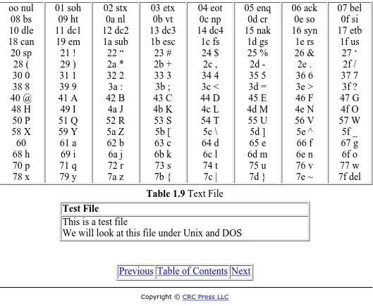
1.3 Character Formats—ASCII

(35)

while the Unix file uses only a new line. As a result Unix text files will be smaller than DOS text files. In the DOS and Unix tables, underneath each character is its ASCII representation in hex. The numbering on the left of each table is the offset in octal of the line in the file.

(36)

Example 1.3 Converting 0.4 from Decimal to Binary

(37)

(38)

(39)

(40)

[image:40.612.44.573.20.455.2]

oo nul 08 bs 10 dle 18 can 20 sp 28 ( 30 0 38 8 40 @ 48 H 50 P 58 X 60 68 h 70 p 78 x 01 soh 09 ht 11 dc1 19 em 21 ! 29 ) 31 1 39 9 41 A 49 I 51 Q 59 Y 61 a 69 i 71 q 79 y 02 stx 0a nl 12 dc2 1a sub 22 “ 2a * 32 2 3a : 42 B 4a J 52 R 5a Z 62 b 6a j 72 r 7a z 03 etx 0b vt 13 dc3 1b esc 23 # 2b + 33 3 3b ; 43 C 4b K 53 S 5b [ 63 c 6b k 73 s 7b { 04 eot 0c np 14 dc4 1c fs 24 $ 2c , 34 4 3c < 44 D 4c L 54 T 5c \ 64 d 6c l 74 t 7c | 05 enq 0d cr 15 nak 1d gs 25 % 2d -35 5 3d = 45 E 4d M 55 U 5d ] 65 e 6d m 75 u 7d } 06 ack 0e so 16 syn 1e rs 26 & 2e . 36 6 3e > 46 F 4e N 56 V 5e ^ 66 f 6e n 76 v 7e ~ 07 bel 0f si 17 etb 1f us 27 ‘ 2f / 37 7 3f ? 47 G 4f O 57 W 5f _ 67 g 6f o 77 w 7f del

Table 1.9 Text File

Test File

This is a test file

We will look at this file under Unix and DOS

(41)

by Alan Parker

ISBN: 0849371716 Pub Date: 08/01/93

1.4 Putting it All Together

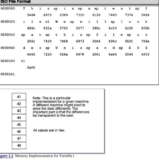
This section presents an example combining ASCII, floating point, and integer types using one final C++ program. The program is shown in Code List 1.15 and the output is shown in Code List 1.16.

The program utilizes a common memory location to store 8 bytes of data. The data will be treated as double, float, char, int, or long. A particular memory implementation for this program is shown in Figure 1.2.

Table 1.10 DOS File Format

(42)

[image:42.612.20.564.36.603.2]

(43)

Figure 1.3 Mapping of each Union Entry

The organization of each union entry is shown in Figure 1.3. For the union declaration t there are only eight bytes stored in memory. These eight bytes can be interpreted as eight individual characters or two longs or two doubles, etc. For instance by looking at Table 1.8 one sees the value of ch[0] which is 0×41 which is the letter A. Similarly, the value of ch[1] is 0×42 which is the letter B. When interpreted as an integer the value of i[0] is 0×41424344 which is in 2’s complement format. Converting to decimal one has i[0] with the value of

If one were to interpret 0×41424344 as an IEEE 32-bit floating point number its value would be 12.1414. If one were to interpret 0×45464748 as an IEEE 32-bit floating point number its value would be 3172.46.

(44)

(45)

There are only one’s and zero’s stored in memory and collections of bits can be interpreted to be characters or integers or floating point numbers. To determine which kind of operations to perform the compiler must be able to determine the type of each operation.

1.5 Problems

(1.1) Represent the following decimal numbers when possible in the format specified. 125, -1000, 267, 45,

0, 2500. Generate all answers in HEX!

a) 8-bit 2’s complement—2 hex digits b) 16-bit 2’s complement—4 hex digits c) 32-bit 2’s complement—8 hex digits d) 64-bit 2’s complement—16 hex digits

(1.2) Convert the 12-bit 2’s complement numbers that follows to 32-bit 2’s complement numbers. Present

your answer with 8 hex digits.

(46)

(1.3) Represent decimal 0.35 in IEEE 32-bit format and IEEE 64-bit format. (1.4) Represent the decimal fraction 4/7 in binary.

(1.5) Represent the decimal fraction 0.3 in octal. (1.6) Represent the decimal fraction 0.85 in hex.

(1.7) Calculate the floating point number represented by the IEEE 32-bit representation F8080000. (1.8) Calculate the floating point number represented by the IEEE 64-bit representation

F808000000000000.

(1.9) Write down the ASCII representation for the string “Hello, how are you?”. Strings in C++ are

terminated with a 00 in hex (a null character). Terminate your string with the null character. Do not represent the quotes in your string. The quotes in C++ are used to indicate the enclosure is a string.

(1.10) Write a C++ program that outputs “Hello World”.

(1.11) In Code List 1.8 the twos complement of the largest representable negative integer, -32768, is the

same number. Explain this result. Is the theory developed incorrect?

(1.12) In Section 1.1.4 the issue of conversion is assessed for signed-magnitude, unsigned, and 2’s

complement numbers. Is there a simple algorithm to convert an IEEE 32-bit floating point number to IEEE 64-bit floating point number?

(47)

by Alan Parker

ISBN: 0849371716 Pub Date: 08/01/93

Chapter 2 Algorithms

This chapter presents the fundamental concepts for the analysis of algorithms.

2.1 Order

N denotes the set of natural numbers, {1, 2, 3, 4, 5, . . .}.

Definition 2.1

A sequence, x, over the real numbers is a function from the natural numbers into the real numbers:

x₁ is used to denote the first element of the sequence, x(1) In general,

and will be written as

Unless otherwise noted, when x is a sequence and f is a function of one variable, f(x), is the sequence obtained by applying the function f to each of the elements of x. If

then

(48)

Definition 2.2

If x and y are sequences, then x is of order at most y, written x O (y), if there exists a positive integer N and a positive number k such that

Definition 2.3

If x and y are sequences then x is of order exactly y, written, x ˜ ( y), if x ˜ ( y) and y O (x).

Definition 2.4

If x and y are sequences then x is of order at least y, written, x © ( y), if y O (x).

Definition 2.5

The time complexity of an algorithm is the sequence

(49)

Example 2.1 Time Complexity

The calculation of the time complexity for addition is illustrated in Example 2.1. A comparison of the order of several classical functions is shown in Table 2.1. The time required for a variety of operations on a 100 Megaflop machine is illustrated in Table 2.2. As can be seen from Table 2.1 if a problem is truly of exponential order then it is unlikely that a solution will ever be rendered for the case of n=100. It is this fact that has led to the use of heuristics in order to find a “good solution” or in some cases “a solution” for problems thought to be of exponential order. An example of Order is shown in Example 2.2. through Example 2.4.

(50)

Function n=1 n=10 n=100 n=1000 n=10000

log(n) 0 3.32 6.64 9.97 13.3

nlog (n) 0 33.2 664 9.97×103 _1.33×105

n2 ₁ ₁₀₀ ₁₀₀₀₀ _1×106 _1×108

n5 ₁ _1×105 _1×1010 _1×1015 _1×1020

en _2.72 _2.2×104 _2.69×1043 _1.97×10434 _8.81×104342

n! 1 3.63×106 _9.33×10157 _4.02×102567 _2.85×1035659

Table 2.2 Calculations for a 100 MFLOP machine

Time # of Operations

1 second 108

1 minute 6×109

1 hour 3.6×1011

1 day 8.64×1012

1 year 3.1536×1015

1 century 3.1536×1017

100 trillion years 3.1536×1029

2.1.1 Justification of Using Order as a Complexity Measure

One of the major motivations for using Order as a complexity measure is to get a handle on the inductive growth of an algorithm. One must be extremely careful however to understand that the definition of Order is “in the limit.” For example, consider the time complexity functions f₁ and f₂ defined in Example 2.6. For these functions the asymptotic behavior is exhibited when n e 1050_{. Although f}

1 ˜ ( en) it has a

value of 1 for n < 1050_{. In a pragmatic sense it would be desirable to have a problem with time}

complexity f₁ rather than f₂. Typically, however, this phenomenon will not appear and generally one might assume that it is better to have an algorithm which is ˜ (1) rather than ˜ (en_{). One should always}

(51)

(52)

Example 2.3 Order

(53)

by Alan Parker

ISBN: 0849371716 Pub Date: 08/01/93

2.2 Induction

Simple induction is a two step process:

• Establish the result for the case N = 1

• Show that if is true for the case N = n then it is true for the case N = n+1

This will establish the result for all n > 1.

Induction can be established for any set which is well ordered. A well-ordered set, S, has the property that if

then either

(54)

Additionally, if S2 is a nonempty subset of S:

then S2 has a least element. An example of simple induction is shown in Example 2.5.

(55)

(56)

Example 2.5 Induction

1. Let P (k) = TRUE denote that a property holds for the value of k. Also assume that P(0) does

not hold so P(0) = FALSE. Let S be the set that

From the well-ordering principle it is true that if S is not empty then S has a smallest member. Let j be such a member:

2. Prove that P(j) implies P(j-1) and this will lead to a contradiction since P(0) is FALSE and j

was assumed to be minimal so that S must be empty. This implies the property does not hold for any positive integer k. See Problem 2.1 for a demonstration of infinite descent.

2.3 Recursion

Recursion is a powerful technique for defining an algorithm.

Definition 2.6

A procedure is recursive if it is, whether directly or indirectly, defined in terms of itself.

2.3.1 Factorial

One of the simplest examples of recursion is the factorial function f(n) = n!. This function can be defined recursively as

A simple C++ program implementing the factorial function recursively is shown in Code List 2.1. The output of the program is shown in Code List 2.2.

(57)

2.3.2 Fibonacci Numbers

(58)

A simple program which implements the Fibonacci sequence recursively is shown in Code List 2.3. The output of the program is shown in Code List 2.4.

Code List 2.3 Fibonacci Sequence Generation

(59)

The recursive implementation need not be the only solution. For instance in looking for a closed solution to the relation if one assumes the form F (n) = »n_{one has}

which assuming » ` 0

The solution via the quadratic formula yields

Because Eq. 2.7 is linear it admits solutions of the form

(60)

multiplying both sides by the 2 × 2 matrix inverse

which yields

resulting in the closed form solution

A nonrecursive implementation of the Fibonacci series is shown in Code List 2.5. The output of the program is the same as the recursive program given in Code List 2.4.

(61)

2.3.3 General Recurrence Relations

This section presents the methodology to handle general 2nd order recurrence relations. The recurrence relation given by

with initial conditions:

can be solved by assuming a solution of the form R (n) = »n_{. This yields}

If the equation has two distinct roots, »₁,»₂, then the solution is of the form

(62)

alternate solution is sought:

where » is the double root of the equation. To see that the term C₁n»n_{satisfies the recurrence relation one}

should note that for the multiple root Eq. 2.18 can be written in the form

Substituting C₁n»n_{into Eq. 2.23 and simplifying verifies the solution.}

(63)

by Alan Parker

ISBN: 0849371716 Pub Date: 08/01/93

2.3.4 Tower of Hanoi

The Tower of Hanoi problem is illustrated in Figure 2.1. The problem is to move n discs (in this case, three) from the first peg, A, to the third peg, C. The middle peg, B, may be used to store discs during the transfer. The discs have to be moved under the following condition: at no time may a disc on a peg have a wider disc above it on the same peg. As long as the condition is met all three pegs may be used to complete the transfer. For example the problem may be solved for the case of three by the following move sequence:

where the ordered pair, (x, y), indicates to take a disk from peg x and place it on peg y.

Figure 2.1 Tower of Hanoi Problem

The problem admits a nice recursive solution. The problem is solved in terms of n by noting that to move

n discs from A to C one can move n - 1 discs from A to B move the remaining disc from A to C and then

move the n - 1 discs from B to C. This results in the relation for the number of steps, S (n), required for size n as

(64)

Eq. 2.25 admits a solution of the form

and matching the boundary conditions in Eq. 2.26 one obtains

A growing field of interest is the visualization of algorithms. For instance, one might want to animate the solution to the Tower of Hanoi problem. Each disc move results in a new picture in the animation. If one is to incorporate the pictures into a document then a suitable language for its representation is

PostScript.1_{This format is supported by almost all word processors and as a result is encountered}

frequently. A program to create the PostScript® description of the Tower of Hanoi is shown in Code List 2.6 The program creates an encapsulated postscript file shown in Code List 2.7. The word processor used to generate this book took the output of the program in Code List 2.7 and imported it to yield Figure 2.1! This program illustrates many features of C++.

1_{PostScript® is a trademark of Adobe Systems Inc.}

The program utilizes only a small set of the PostScript® language. This primitive subset is described in Table 2.3.

Table 2.3 PostScript® — Primitive Subset

Command Description

x setgray set the gray level to x.x = 1 is white and x = 0 is black. This will affect the fill operation.

x y scale scale the X dimension by x and scale the Y dimension by y.

x setlinewidth set the linewidth to x.

x y moveto start a subpath and move to location x y on the page.

x y rlineto draw a line from current location (x₁, y₁) to (x₁ + x, y₁ + y). Make the endpoint the current location. Appends the line to the subpath.

fill close the subpath and fill the area enclosed.

newpath create a new path with no current point.

showpage displays the page to the output device.

(65)

function in the object class is void even though for more complex examples it might have a number of operations. The RECTANGLE class inherits all the functions from the GRAPHICS_CONTEXT class and the OBJECT class.

In the program, the rectangle class instantiates the discs, the base, and the pegs. Notice in Figure 2.1 that the base and pegs are drawn in a different gray scale than the discs. This is accomplished by the two calls in main():

• peg.set_gray(0.6) • base.set_gray(0.6)

Any object of type RECTANGLE defaults to a set_gray of 0.8 as defined in the constructor function for the rectangle. Notice that peg is declared as a RECTANGLE and has access to the set_gray function of the GRAPHICS_CONTEXT. The valid operations on peg are:

• peg.set_line_width(), from the GRAPHICS_CONTEXT class • peg.set_scale(), from the GRAPHICS_CONTEXT class • peg.set_gray(), from the GRAPHICS_CONTEXT class • peg.location(), from the OBJECT class

• peg.set_location(), from the RECTANGLE class • peg.set_width(), from the RECTANGLE class • peg.set_height(), from the RECTANGLE class • peg.draw(), from the RECTANGLE class

The virtual function draw in the OBJECT class is hidden from peg but it can be accessed in C++ using the scoping operator with the following call:

• peg.object::draw(), uses draw from the OBJECT class

(66)

by Alan Parker

ISBN: 0849371716 Pub Date: 08/01/93

Hence, in the program, all the functions are available to each instance of the rectangle created. This availability arises because the functions are declared as public in each class and each derived class is also declared public. Without the public declarations C++ will hide the functions of the base class from the derived class. Similarly, the data the functions access are declared as protected which makes the data visible to the functions of the derived classes.

The first peg in the program is created with rectangle peg(80,0,40,180). The gray scale for this peg is changed from the default of 0.8 to 0.6 with peg.set_gray(0.6). The peg is drawn to the file with

peg.draw(file). This draw operation results in the following lines placed in the file:

• newpath • 1 setlinewidth • 0.6 setgray • 80 0 moveto • 0 180 rlineto • 40 0 rlineto • 0 - 180 rlineto • fill

The PostScript® action taken by the operation is summarized in Figure 2.3. Note that the rectangle in the figure is not drawn to scale. The drawing of the base and the discs follows in an analogous fashion.

(67)

(68)

(69)

(70)

(71)

(72)

(73)

(74)

2.3.5 Boolean Function Implementation

This section presents a recursive solution to providing an upper bound to the number of 2-input NAND gates required to implement a boolean function of n boolean variables. The recursion is obtained by noticing that a function, f(x₁,x₂,...,x_n) of n variables can be written as

(75)

The solution to the simple recurrence relation yields, assuming a general form of C(n) = »n_{followed by a}

constant to obtain the particular solution

[image:75.612.35.510.92.429.2]

Applying the boundary condition C (1) = 1 and C (2) = 6 one obtains

Figure 2.4 Recursive Model for Boolean Function Evaluation

2.4 Graphs and Trees

This section presents some fundamental definitions and properties of graphs.

Definition 2.7

A graph is a collection of vertices, V, and associated edges, E, given by the pair

(76)

Figure 2.5 A Simple Graph

Definition 2.8

The size of a graph is the number of edges in the graph

Definition 2.9

The order of a graph G is the number of vertices in a graph

For the graph in Figure 2.5 one has

Definition 2.10

The degree of a vertex (also referred to as a node), in a graph, is the number of edges containing the vertex.

Definition 2.11

In a graph, G = (V, E), two vertices, v₁ and v₂, are neighbors if

(v₁,v₂) E or (v₁,v₂) E

(77)

Definition 2.12

If G = (V₁, E₁) is a graph, then H = (V₂, E₂) is a subgraph of G written if and .

[image:77.612.19.463.125.347.2]

A subgraph of the graph in Figure 2.5 is shown in Figure 2.6.

Figure 2.6 Subgraph of Graph in Figure 2.5

The subgraph is generated from the original graph by the deletion of a single edge (v₂, v₃).

Definition 2.13

A path is a collection of neighboring vertices.

For the graph in Figure 2.5 a valid path is

Definition 2.14

A graph is connected if for each vertex pair (v_i,v_j) there is a path from v_i to v_j.

The graph in Figure 2.5 is connected while the graph in Figure 2.6 is disconnected.

Definition 2.15

A directed graph is a graph with vertices and edges where each edge has a specific direction relative to each of the vertices.

(78)

[image:78.612.44.493.52.355.2]

Figure 2.7 A Directed Graph

The graph in the figure has G = (V, E) with

In a directed graph the edge (v_i, v_j) is not the same as the edge (v_j, v_i) when i ` j. The same terminology G = (V, E) will be used for directed and undirected graphs; however, it will always be stated whether the graph is to be interpreted as a directed or undirected graph.

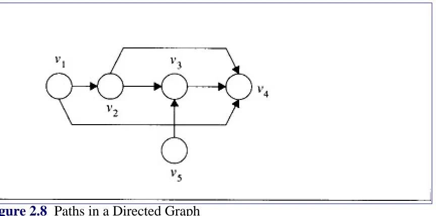
The definition of path applies to a directed graph also. As shown in Figure 2.8 there is a path from v₁ to

v₄ but there is no path from v₂ to v₅.

Figure 2.8 Paths in a Directed Graph

[image:78.612.24.456.465.679.2]

(79)

(80)

by Alan Parker

ISBN: 0849371716 Pub Date: 08/01/93

Definition 2.16

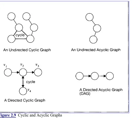
A cycle is a path from a vertex to itself which does not repeat any vertices except the first and the last.

[image:80.612.16.469.270.675.2]

A graph containing no cycles is said to be acyclic. An example of cyclic and acyclic graphs is shown in Figure 2.9.

Figure 2.9 Cyclic and Acyclic Graphs

Notice for the directed cyclic graph in Figure 2.9 that the double arrow notations between nodes v₂ and v₄ indicate the presence of two edges (v₂, v₄) and (v₄, v₂). In this case it is these edges which form the cycle.

(81)

A tree is an acyclic connected graph.

Examples of trees are shown in Figure 2.10.

Definition 2.18

[image:81.612.32.493.131.499.2]

An edge, e, in a connected graph, G = (V, E), is a bridge if G2 = (V, E2) is disconnected where

Figure 2.10 Trees

If the edge, e, is removed, the graph, G, is divided into two separate connected graphs. Notice that every edge in a tree is a bridge.

Definition 2.19

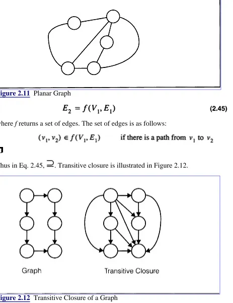
A planar graph is a graph that can be drawn in the plane without any edges intersecting.

An example of a planar graph is shown in Figure 2.11. Notice that it is possible to draw the graph in the plane with edges that cross although it is still planar.

Definition 2.20

(82)

[image:82.612.18.481.67.669.2]

Figure 2.11 Planar Graph

where f returns a set of edges. The set of edges is as follows:

Thus in Eq. 2.45, . Transitive closure is illustrated in Figure 2.12.

(83)

2.5 Parallel Algorithms

This section presents some fundamental properties and definitions used in parallel processing.

2.5.1 Speedup and Amdahls Law

Definition 2.21

The speedup of an algorithm executed using n parallel processors is the ratio of the time for execution on a sequential machine, T_SEQ, to the time on the parallel machine, T_PAR:

If an algorithm can be completely decomposed into n parallelizable units without loss of efficiency then the Speedup obtained is

If however, only a fraction, f, of the algorithm is parallelizable then the speedup obtained is

which yields

This is known as Amdahl's Law. The ratio shows that even with an infinite amount of computing power an algorithm with a sequential component can only achieve the speedup in Eq. 2.50. If an algorithm is 50% sequential then the maximum speedup achievable is 2. While this may be a strong argument against the merits of parallel processing there are many important problems which have almost no sequential components.

Definition 2.22

(84)

Using Amdahl's law

with

2.5.2 Pipelining

Pipelining is a means to achieve speedup for an algorithm by dividing the algorithm into stages. Each stage is to be executed in the same amount of time. The flow is divided into k distinct stages. The output of the jth stage becomes the input to the (j + 1) th stage. Pipelining is illustrated in Figure 2.13. As seen in the figure the first output is ready after four time steps Each subsequent output is ready after one additional time step. Pipelining becomes efficient when more than one output is required. For many algorithms it may not be possible to subdivide the task into k equal stages to create the pipeline. When this is the case a performance hit will be taken in generating the first output as illustrated in Figure 2.14.

(85)

[image:85.612.33.510.43.300.2]

Figure 2.14 Pipelining

In the figure T_SEQ is the time for the algorithm to execute sequentially. T_PS is the time for each pipeline stage to execute. T_PIPE is the time to flow through the pipe. The calculation of the time complexity sequence to process n inputs yields

for a k-stage pipe. It follows that T_PIPE (n) < T_SEQ (n) when

(86)

which yields

In some applications it may not be possible to keep the pipeline full at all times. This can occur when there are dependencies on the output. This is illustrated in Example 2.7. For this case let us assume that the addition/subtraction operation has been set up as a pipeline. The first statement in the pseudo-code will cause the inputs x and 3 to be input to the pipeline for subtraction. After the first stage of the pipeline is complete, however, the next operation is unknown. In this case, the result of the first statement must be established. To determine the next operation the first operation must be allowed to proceed through the pipe. After its completion the next operation will be determined. This process is referred to flushing the pipe. The speedup obtained with flushing is demonstrated in Example 2.8.

(87)

Example 2.8 Pipelining

2.5.3 Parallel Processing and Processor Topologies

There are a number of common topologies used in parallel processing. Algorithms are increasingly being developed for the parallel processing environment. Many of these topologies are widely used and have been studied in great detail. The topologies presented here are

• Full Crossbar • Rectangular Mesh • Hypercube

• Cube-Connected Cycles

(88)

by Alan Parker

ISBN: 0849371716 Pub Date: 08/01/93

2.5.3.1 Full Crossbar

[image:88.612.17.479.251.532.2]

A full crossbar topology provides connections between any two processors. This is the most complex connection topology and requires (n (n - 1) / 2 connections. A full crossbar is shown in Figure 2.15. In the graphical representation the crossbar has the set, V, and E with

Figure 2.15 Full Crossbar Topology

Because of the large number of edges the topology is impractical in design for large n.

2.5.3.2 Rectangular Mesh

A rectangular mesh topology is illustrated in Figure 2.16. From an implementation aspect the topology is easily scalable. The degree of each node in a rectangular mesh is at most four. A processor on the interior of the mesh has neighbors to the north, east, south, and west. There are several ways to implement the exterior nodes if it is desired to maintain that all nodes have the same degree. For an example of the external edge connection see Problem 2.5.

2.5.3.3 Hypercube

(89)

each node increases. The magnitude of the increase is clearly more manageable than that of the full

crossbar but it can still be a significant problem with hypercube architectures containing 64K nodes. As a result the cube-connected cycles, described in the next section, becomes more attractive due to its fixed degree.

[image:89.612.24.494.115.369.2]

The vertices of an n dimensional hypercube are readily described by the binary ordered pair

Figure 2.16 Rectangular Mesh

With this description two nodes are neighbors if they differ in their representation in one location only. For example for an 8 node hypercube with nodes enumerated

(90)

[image:90.612.21.463.429.739.2]

Figure 2.17 Hypercube Topology

2.5.3.4 Cube-Connected Cycles

(91)

Figure 2.18 Cube-Connected Cycles

2.6 The Hypercube Topology

This section presents algorithms and issues related to the hypercube topology. The hypercube is important due to its flexibility to efficiently simulate topologies of a similar size.

2.6.1 Definitions

Processors in a hypercube are numbered 0, ..., n - 1. The dimension, d, of a hypercube, is given as

where at this point it is assumed that n is a power of 2. A processor, x, in a hypercube has a representation of

For a simple example of the enumeration scheme see Section 2.5.3.3 on page 75. The distance, d (x, y), between two nodes x and y in a hypercube is given as

The distance between two nodes is the length of the shortest path connecting the nodes. Two processors, x and y are neighbors if d (x, y) = 1. The hypercubes of dimension two and three are shown in Figure 2.19.

2.6.2 Message Passing

A common requirement of a parallel processing topology is the ability to support broadcast and message passing algorithms between processors. A broadcast operation is an operation which supports a single processor communicating information to all other processors. A message passing algorithm supports a single message transfer from one processor to the next. In all cases the messages are required to traverse the edges of the topology.

(92)

[image:92.612.81.456.208.715.2]

(93)

In general, in a hypercube of dimension d, a message travelling from processor x to processor y has d (x,

y) ! distinct paths (see Problem 2.11). One simple algorithm is to compute the exclusive-or of the source

and destination processors and traverse the edge corresponding to complementing the first bit that is set. This is illustrated in Table 2.4 for left to right complementing and in Table 2.5 for right to left

complementing.

Table 2.4 Calculating the Message Path — Left to Right

Processor Source ProcessorDestination Exclusive-Or Next Processor

000 111 111 100

100 111 011 110

110 111 001 111

Table 2.5 Calculating the Message Path — Right to Left

Processor Source Processor Destination Exclusive-Or Next Processor

000 111 111 001

001 111 110 011

011 111 100 111

The message passing algorithm still works under certain circumstances even when the hypercube has nodes that are faulty. This is discussed in the next section.

2.6.3 Efficient Hypercubes

This section presents the analysis of the class of hypercubes for which the message passing routines of the previous section are valid. Examples are presented in detail for an 8-node hypercube.

2.6.3.1 Transitive Closure

Definition 2.23

The adjacency matrix, A, of a graph, G, is the matrix with elements a_ij such that a_ij = 1 implies there is an edge from i to j. If there is no edge then a_ij = 0.

(94)

For a hypercube with all functional nodes every processor is reachable.

(95)

by Alan Parker

ISBN: 0849371716 Pub Date: 08/01/93

2.6.3.2 Least-Weighted Path-Length

Definition 2.24

The least-weighted path-length graph is the directed graph where the weights of each edge correspond to the shortest path-length between the nodes.

The associated weighted matrix consists of the path-length between the nodes. The path-length between a processor and itself is defined to be zero. The associated weighted matrix for an 8-node hypercube with all functional nodes is

a_ij is the distance between nodes i and j. If nodes i and j are not connected via any path then a_ij = .

2.6.3.3 Hypercubes with Failed Nodes

This section introduces the scenario of failed processors. It is assumed if a processors or node fails then all edges incident on the processor are removed from the graph. The remaining processors will attempt to function as a working subset while still using the message passing algorithms of the previous sections. This will lead to a characterization of subcubes of a hypercube which support message passing. Consider the scenario illustrated in Figure 2.20. In the figure there are three scenarios with failed processors.

In Figure 2.20b a single processor has failed. The remaining processors can communicate with each other using a simple modification of the algorithm which traverses the first existing edge encountered.

(96)

[image:96.612.29.453.39.545.2]

Figure 2.20 Hypercube with Failed Nodes

Table 2.6 Calculating the Message Path — Right to Left for Figure 2.20c

000 111 111 010

010 111 101 011

011 111 100 111

The scenario in Figure 2.20d is quite different. This is illustrated in Table 2.7.

(97)

Notice that the distance between the processors has increased as a result of the two processors failures. This attribute is the motivation for the characterization of efficient hypercubes in the next section.

Table 2.7 Calculating the Message Path — Right to Left for Figure 2.20d

000 011 011 ?

2.6.3.4 Efficiency

Definition 2.25

A subcube of a hypercube is efficient if the distance between any two functional processors in the subcube is the same as the distance in the hypercube.

A subcube with this property is referred to as an efficient hypercube. This is equivalent to saying that if A represents the least-weighted path-length matrix of the hypercube and B represents the least-weighted path-length matrix of the efficient subcube then if i and j are functional processors in the subcube then b_ij = a_ij. This elegant result is proven in Problem 2.20. The least-weighted path-length matrix for efficient hypercubes place in column i and row i if processor i is failed.

The cubes in Figure 2.20b and c are efficient while the cube in Figure 2.20d is not efficient. If the cube is efficient then the modified message passing algorithm in the previous section works. The next section implements the procedure for hypercubes with failed nodes.

2.6.3.5 Message Passing in Efficient Hypercubes

The code to simulate message passing in an efficient hypercube is shown in Code List 2.8. The output of the program is shown in Code List 2.9. The path for communicating from 0 to 63 is given as

0-1-3-7-15-31-63 as shown in Code List 2.9. Subsequently processor 31 is deactivated and a new path is calculated as 0-1-3-7-15-47-63 which avoids processor 31 and traverses remaining edges in the cube. The program continues to remove nodes from the cube and still calculates the path. All the subcubes created result in an efficient subcube.

(98)

(99)

(100)

(101)

2.6.4 Visualizing the Hypercube: A C++ Example

This section presents a C++ program to visualize the hypercube. A program to visualize the cube is shown in Code List 2.10. The program was used to generate the PostScript image in Figure 2.21 for a 64 node hypercube. The program uses a class structure similar to the program to visualize the Tower of Hanoi in Code List 2.6.

The program introduces a new PostScript construct to draw and fill a circle

(102)

The program uses the scale operator to force the image to fill a specified area. To illustrate this, notice that the program generated both Figure 2.21 and Figure 2.22. The nodes in Figure 2.22 are enlarged via the scale operator while the nodes in Figure 2.21 are reduced accordingly.

[image:102.612.23.444.123.548.2]

The strategy in drawing the hypercube is such that only at most two processors appear in any fixed horizontal or vertical line. The cube is grown by replications to the right and downward.

Figure 2.21 A 64-Node Hypercube

(103)

[image:103.612.20.452.90.636.2]

(104)

(105)

(106)

(107)

(108)

(109)

(110)

(111)

(112)

(113)

(114)

by Alan Parker

ISBN: 0849371716 Pub Date: 08/01/93

2.7 Problems

(2.1) [Infinite Descent — Difficult] Prove, using infinite descent, that there are no solutions in the

positive integers to

(2.2) [Recuffence] Find the closed form solution to the recursion relation

and write a C++ program to calculate the series via the closed form solution and print out the first twenty terms of the series for

(2.3) [Tower of Hanoi] Write a C++ Program to solve the Tower of Hanoi problem for arbitrary n.

This program should output the move sequence for a specific solution.

(2.4) [Tower of Hanoi] Is the minimal solution to the Tower of Hanoi problem unique? Prove or

disprove your answer.

(2.5) [Rectangular Mesh] Given an 8x8 rectangular mesh with no additional edge connections

calculate the largest distance between two processors, where the distance is defined as the minimum number of edges to traverse in a path connecting the two processors.

(2.6) [Rectangular Mesh] For a rectangular mesh with no additional edge connections formally

describe the topology in terms of vertices and edges.

(2.7) [Rectangular Mesh] Write a C++ program to generate a PostScript image file of the

rectangular mesh for 1 d n d 20 without additional external edge connections. To draw a line from the current point to (x, y) use the primitive