Spot Transit: Cheaper Internet Transit for Elastic Traffic

(1)

IEEE TRANSACTIONS ON SERVICES COMPUTING, 201X 1

Spot Transit: Cheaper Internet Transit

for Elastic Traffic

Hong Xu,

Member, IEEE,

and Baochun Li,

Senior Member, IEEE

Abstract—We advocate to create aspotInternet transit market, where transit is sold using the under-utilized backbone capacity at a lower price. The providers can improve profit by capitalizing the perishable capacity, and customers can buy transit on demand without a minimum commitment level for elastic traffic, and as a result improve their surplus (i.e., utility gains). We conduct a systematic study of the economical benefits of spot transit both theoretically and empirically. We propose a simple analytical framework with a general demand function, and solve the pricing problem to maximize the expected profit, taking into account the potential revenue loss of regular transit when spot transit traffic hikes. We prove the price advantage of spot transit, as well as the profit and surplus improvements for tier-1 ISPs and customers, respectively. Using real-world price data and traffic statistics of 6 IXPs with more than 1000 ISPs, we evaluate spot transit and show that significant financial benefits can be achieved in both absolute and relative terms, robust to parameter values.

Index Terms—Network economics, Internet transit, bandwidth pricing

F

1 I

NTRODUCTION

Internet transit has traditionally been traded with long-term contracts, where the tier-1 Internet Ser-vice Provider (ISP) specifies pricing and the transit customers commit a minimum level of bandwidth consumption. Two facts make this market inefficient for today’s Internet. First, tier-1 ISPs typically over-provision the backbone and have a portion of the capacity under-utilized most of the time [13], which represents a bulk of the missing revenue opportunities. Second, the transit customers are increasingly unwill-ing to purchase transit due to sheer costs of servunwill-ing the ever increasing traffic volumes. Cisco estimates that busy-hour Internet traffic will increase fivefold by 2015 while average traffic will increase fourfold [12].

In this paper, we advocate that aspotInternet transit

market should be created, where the unused transit capacity is sold at a lower price to compliment the traditional contract-based market. To serve the spot traffic, the tier-1 ISP uses its under-utilized capacity that are otherwise wasted. It provides no Quality-of-Service (QoS) guarantee or support for spot transit. This enables the ISP to adopt a lower price and earn extra revenue from the available, yet perishable, band-width resource. It can also stop routing the spot traffic at any time, when capacity is needed for regular transit or to handle network failures.

The transit customers, on the other hand, have the

flexibility to buy transiton demandat a discount. Spot

transit is ideal for elastic traffic [33]. For example, data

• Hong Xu is with Department of Computer Science, City University of Hong Kong, Kowloon, Hong Kong. Email: [email protected]. Baochun Li is with Department of Electrical and Computer Engineer-ing, University of Toronto, Toronto, Ontario M5S 3G4, Canada. Email: [email protected].

centers can use it for the bulk backup and replication traffic across the Internet [11], [19]. Eyeball ISPs can use it at demand valleys to support time-dependent pricing [16]. A lower broadband access price can be advertised at valley periods, encouraging users to de-fer time-insensitive applications, and reduce the costly peak demand. In short, they can cope with traffic fluctuations in a more flexible and cost efficient way.

Moreover, small ISPs that originally rely on various forms of peering or buying from transit resellers [35], [39] can now purchase spot transit to offload the elastic traffic, and enjoy the reachability of a tier-1 backbone with lower costs. The barrier of minimum committed data rates no longer exists. Since it does not differentiate based on protocol or user type, spot transit is also less susceptible to network neutrality concerns spawned by some instances of paid peering [1], [39].

In this paper, we are primarily interested in the economic aspect of the market, in particular, pricing, profit for tier-1 ISPs, and consumer surplus, i.e. utility gains, for transit customers. Pricing is critical as it di-rectly affects the incentives of both sides to participate. We take the liberty to envision that a spot market is technically feasible, and conduct a systematic study of the economical benefits of spot transit.

The unique challenge of pricing here arises from an intriguing interplay between the spot and regular transit traffic, whose bits share the same backbone infrastructure. When the tier-1 ISP tries to lower the price to attract demand, it is certainly possible that the increased spot traffic hogs up the network and causes performance degradation to the regular traffic.

Therefore, the risk of demand overflow and its impact

on profit have to be taken into account.

We solve the spot transit pricing problem for ex-pected profit maximization of a tier-1 ISP under the

(2)

classical additive random demand model [31], which we validate against real inter-domain traffic. Further, we prove that spot transit improves both profit and consumer surplus, as long as it is cheaper than regular transit. It is therefore a win-win solution for both sides. We emphasize that all our results are obtained with a general demand function that captures the basic

prop-erties ofanydemand function. Essentially, the benefits

of spot transit only depend on the characteristics of elastic traffic.

To quantitatively understand the potential of spot transit, we perform an extensive empirical evaluation based on traffic traces collected from 6 Internet eX-change Points (IXPs) in America, Europe, and Asia. The dataset of each IXP contains aggregated traffic statistics from more than 100 ISPs with peak demand between 1200 Gbps and around 200 Gbps. We use two canonical demand functions with real transit prices, empirical demand elasticity data, and a range of model parameters. We find that, spot transit typically can be 15%-30% cheaper, and provide more than 60% profit improvement for tier-1 ISPs and more than 10% sur-plus improvement for customers. In dollar terms, the profit and surplus gains are on the order of millions (monthly) for large IXPs and hundreds of thousands for smaller ones. The benefit is robust: 10% profit and surplus improvements are still observed even in the worst case.

We make three original contributions in this paper. First, we propose spot transit, a transit market that allows customers to buy underutilized transit capacity on demand at a discounted price (Sec. 2). Second, we propose a simple analytical framework that strikes a balance between economic theory and realistic aspects of Internet transit. With a general demand function (Sec. 3), we characterize the optimal price as a function of the provision cost, overflow penalty, demand elas-ticity, and the predictability of traffic. We theoretically establish the price advantage and efficiency gains of spot transit (Sec. 4). Third, we empirically evaluate spot transit using real traffic statistics and price data. We obtain realistic parameters for demand functions by fitting empirical traffic data into canonical economic models, and demonstrate the significant benefits of spot transit (Sec. 5). Towards the end, we also discuss issues about implementing such a market (Sec. 6).

2 B

ACKGROUND AND

M

OTIVATION

The Internet backbone consists of a small number of tier-1 ISPs, each owning a portion of the global infras-tructure, and can reach the entire Internet solely via

settlement-free interconnection, i.e. peering. They

pro-vide transit services to transit customers for monetary

returns. It is widely known that the tier-1 backbone is largely under-utilized (under 50%) due to over-provisioning [13]. Over recent years, though traffic has been growing at a 40%–50% annual rate [12], [18], backbone capacity has been increasing worldwide at

an equivalent pace [37]. As a result, underutilization continues, with average and peak link utilization on major backbone lines virtually unchanged [36].

The under-utilized backbone capacity represents a bulk of missing revenue opportunities for tier-1 ISPs.

Network capacity is inherently a perishable resource:

bandwidth that is not used is lost forever. On the other hand, despite the constant decline of transit prices [37], customers face enormous transit costs due to the rapid-growing traffic. New forms of peering [39] and smart traffic engineering schemes [19], [40] are continuously being developed to cut the transit bill. This demonstrates the inefficiency of the current market, and calls for novel solutions that offer better ways of trading transit.

Motivated by these observations, we propose to

create aspottransit market, where the unused capacity

is sold at a discount without SLAs regarding network availability, route stability, etc. Transit customers can purchase spot transit on-demand without entering a contract first. The spot transit market compliments the regular contract based market. It suits well to serve the elastic traffic, such as the bulk replication and backup traffic across datacenters and most residential broadband traffic, because it can tolerate delay and loss and is much more price sensitive [39].

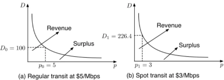
D p p0= 5 p1= 3 D0= 100 D1= 226.4 D p Surplus Surplus Revenue Revenue

(a) Regular transit at $5/Mbps (b) Spot transit at $3/Mbps Fig. 1. The benefits of the spot transit market. It improves the social welfare by improving the revenue for tier-1 ISPs, and surplus for transit customers. The demand curve shown isD= 1313.26·p 1.6_.

To intuitively see the potential of the spot transit market, Figure 1 shows a typical iso-elastic demand curve [24], [39] for a tier-1 ISP’s elastic traffic. We choose the demand function such that at a regular transit price of $5/Mbps, the elastic traffic is 100 Gbps. The revenue is $500,000 per month. If the demand were to be served by the spot transit market, since the tier-1 ISP does not need to provide QoS guarantees, it can afford a lower price of, say, $3/Mbps, with a 40% discount. At such a low price, demand rises to around 226.4 Gbps, and our tier-1 ISP collects around $680,000. Thus, by creating the spot transit market and optimizing price, the tier-1 ISP attains a 36% profit increase. This represents a strong financial incentive.

The spot transit market also benefits transit cus-tomers in terms of consumer surplus, which is the difference between the total amount that they are willing to pay and the actual amount that they do pay at the market price [22]. As depicted in Figure 1,

(3)

consumer surplus is greatly improved with a lower transit price.

Therefore, the spot market achieves higher efficiency and improves social welfare. The underlying reason is that in the conventional transit market, elastic traffic is priced together with inelastic traffic that has higher costs to serve. By pricing the elastic traffic separately with spot transit that has no SLAs, tier-1 ISPs are able to adopt a lower price, which in turns attracts even more demand and increases profit.

The demand increase with spot transit can be ex-plained by at least two factors: competition with peer-ing and transit resellpeer-ing. The low price and on-demand feature of spot transit can make it more appealing than peering or paid peering, considering the performance benefits and network reachability provided by the tier-1 backbone. Further, small ISPs usually find it difficult to purchase transit directly from tier-1 ISPs due to the minimum committed data rate requirement, and rely on transit resellers instead. With spot transit, tier-1 ISPs are able to collect additional profits from these small ISPs by bypassing the transit resellers in the middle. In all, we expect that spot transit compliments the traditional transit business of a tier-1 ISP.

3 M

ODEL

In this section, we introduce the theoretical model for our analysis of the optimal pricing, and the benefits of spot transit.

3.1 Spot transit market

We consider a spot transit market with multiple tier-1 ISPs. This corresponds to an oligopoly scenario. Numerous game models can be adopted [22] and each considers specific competition scenarios. Our objective is to study spot transit under a general model that captures the key aspects of the market. For the appli-cability of results and ease of exposition, we choose to

focus on a representative tier-1 ISP, with the residual

demand that is not met by other competitors in the market. Residual demand is a common concept in microeconomics in studying the pricing problem for a firm operating in a competitive market [24], [39].

Though residual demand does not model the full dynamic interactions between ISPs, it accounts for the availability of substitutes and switching costs. It also allows a faithful empirical verification, since the real-world price and demand data collected reflect the effect of competition. The same approach is also adopted in [39].

3.2 Demand

One of the challenges of conducting economic analysis in networking is the lack of a good model for the resid-ual demand, or simply demand, in general. Not much public information is known about the Internet transit market in particular for business reasons. Here we

Fig. 2. Weekly and monthly aggregated traffic at NIX, an Internet exchange in Czech Republic [26].

blend theory with practice, and use classical demand models from economics with empirical justifications based on real traffic data. We believe such an approach not only makes the analysis tractable, but also the results practically relevant.

3.2.1 A model for billable demand

We define spot transit demandDas the actualbillable

amount of bandwidth, i.e. the 95-percentile demand. Other pricing schemes, such as volume pricing, can be studied in a similar way. The aggregated traffic of a tier-1 ISP often exhibits a diurnal pattern with high predictability [13], [30]. For example Figure 2 plots the aggregated traffic at the Neutral Internet eXchange (NIX) in Czech Republic [26]. The diurnal pattern is clearly visible in both weekly and monthly scales. Nat-urally, one can thus employ statistical methods over traffic time series to estimate the billable demand, with a small error that arises from the inherent randomness of demand.

Inspired by this observation, we adopt the classical approach in economics [31] to model the uncertainty of billable demand in an additive fashion. Specifically,

D(p,✏) =d(p) +✏, (1)

following [23]. Here, p is the spot transit price in

$/Mbps, d(p) is the price-dependent demand

func-tion that models the billable demand (more details in

Sec. 3.2.2), and ✏ is a random variable defined over

[A, B]to model the inherent demand uncertainty. Thus

randomness in demand is price independent. That is, the shape of the demand curve is independent of the price, while the mean and variance of the demand distribution are affected by the price. We provide empirical justifications for our demand model using real-world traffic data in Sec. 5.2.

3.2.2 Demand functiond(p)and elasticity

Many demand functions d(p) are valid in economic

analysis. Instead of choosing some specific functions to work with, our analysis assumes a general demand

function. We only require that d(p) is a continuous,

(4)

i.e. d0₍_p₎_< _0, _d00₍_p₎ _{0. Monotonicity and convexity} are general characteristics of the demand-price inter-action. These assumptions are quite reasonable and commonly accepted in the literature.

A useful concept related to demand is itselasticity.

Elasticity measures the responsiveness of demand to a

change in price, and is defined at a price pointp as

(p) = p·d0(p)

d(p) . (2)

We can observe that

0₍_p₎ ₀ ₍₃₎

since d0(p) < 0 and d00(p) 0, i.e. elasticity is non-decreasing in p.

Next we show two canonical demand functions that satisfy our assumptions.

Iso-elastic demand.The iso-elastic demand, or

con-stant elasticity demand, is a well-known demand

function derived from the alpha-fair utility function

[24], [39], which is often used to model Internet user activity. As the name suggests, elasticity is constant for every price point.

d(p) =v·p ↵_{, v >}₀_,_↵_>₁_. ₍₄₎

v can be interpreted as the base demand that controls

the magnitude of demand. (p) =↵, where↵ denotes

the constant elasticity: a higher value represents higher elasticity. As discussed above, demand here is the residual demand, and high elasticity can also indicate that the market is more competitive, and substitutes are readily available.

Linear demand. The simple linear function of

de-mand is also popular [22]:

d(p) =v ↵p, v >0,↵>0. (5)

Herevis the base demand. Elasticity of linear demand

is (p) = _v↵p_↵_p. In contrast to iso-elastic demand,

now elasticity decreases in price. Thus it captures the phenomena that sometimes, demand is less sensitive to a price change when the price is already low (recall (3)).

3.3 Surplus, profit, and social welfare

To comprehensively study the economical benefits of

spot transit we consider three metrics, namely

con-sumer surplus, provider profit, andsocial welfare. As we have seen from Figure 1, consumer surplus, or simply surplus is the utility gain obtained by customers due to the purchase of Internet transit. Specifically,

S(p) =

Z 1

p

(x p)d(x)dx. (6)

In other words, the surplus equals the amount cus-tomers are willing to pay, minus the actual cost of

purchase at p. It is evident that S(p) increases as p

decreases, i.e. a price reduction is always beneficial for customers.

Next we characterize provider profit as a function of

the spot transit pricep. We consider the scenario where

the tier-1 ISP allocates a fixed portion of the unused backbone bandwidth to offer spot transit services. This

amount is defined as thecapacityof spot transitC, and

can be safely used without affecting the ISP’s regular

business. A proper choice ofC can be determined by

the ISP profiling its network utilization.

The notion of capacity here is not a rigid resource

constraint. Since demand is inherently random and both the spot and regular transit traffic share the same backbone, nothing prevents the spot traffic from

break-ing through the capacity C and using the capacity

reserved for regular transit. Such a demand overflow

scenario may negatively affect the regular transit traffic and thus the ISP’s revenue. To model the revenue loss,

a penalty of m >0 in $/Mbps is incurred whenever

demand exceeds the capacity, i.e. D(p,✏) > C. An

equivalent interpretation is to treat it as modeling the surplus loss of the regular transit customers due to overflow.m > pC_{, where}_pC_{denotes the price at which} d(p) =C. Thus, the penalty is large enough so that at

the optimal operating point, the expected demand is

smaller thanC.

We let f(·) denote the probability density function

of the demand uncertainty ✏ defined over [A, B]. In

practice ✏ can often be approximated by a Gaussian

random variable. To make sure that positive demand

is possible, we require B < C which holds naturally

since the randomness is small in magnitude compared to capacity. These assumptions will also be verified using real traffic traces in Sec. 5.2.

We can now formally define the spot transit profit. If demand does not exceed the capacity, then profit is simply (p r)D(p,✏), where r > 0 is the unit cost of spot transit. Otherwise the profit consists of a positive component from serving the spot transit and a neg-ative component representing the demand overflow loss, and is written as(p r)D(p,✏) m(D(p,✏) C).

The profit function,R(p,✏)can then be expressed as

R(p,✏) = ⇢

(p r)(d(p) +✏), ✏C d(p)

(p r m)(d(p) +✏) +mC, ✏> C d(p) The expected profit is:

E[R(p)] = (p r)d(p) m Z B C d(p) (d(p) C+u)f(u)du (7) Define (p) = (p r)d(p), and⇤(p) =mR_{C d}B ₍_p₎(d(p)

C+u)f(u)du. (p)represents therisk-freeprofit when demand is deterministic.⇤(p)is the loss function at an

average cost of m when demand overflow happens.

The overall expected profit is the difference between the two.

E[R(p)] = (p) ⇤(p), (8)

Finally, the social welfare of a market is defined as

(5)

the spot transit market, its social welfare (p)is

(p) =S(p) +E[R(p)]. (9)

4 A

N

E

CONOMIC

A

NALYSIS

In this section, we present our analysis on the optimal pricing of spot transit for profit maximization, as well as the resulting profit, surplus and social welfare, to theoretically demonstrate its benefits.

4.1 Pricing for profit maximization

With spot transit, the very first question we need to answer is, how do we price it? Our ISP needs to determine a price to maximize its expected profit with the presence of demand uncertainty, taking into account the risk of demand overflow and its monetary impact. The profit maximization problem can then be formulated:

max

p E[R(p)] (10)

s.t. (7)

For efficient price determination, the optimization problem must have an efficient solution algorithm. The most useful criterion for this property is convexity: minimizing a convex function, or equivalently maxi-mizing a concave function over a convex constraint set. However, we show that this condition is not satisfied for our problem.

Consider the first-order derivative ofE[R(p)], which

can be obtained by applying the Leibniz integral rule:

E0[R(p)] =d(p) +d0(p) p r m·Pr ✏> C d(p) .

(11)

It can be observed that the term in(·)is positive and

decreasing inp, and thus the term (·)d0₍_p₎_is decreas-ing inp. However,d(p) +p·d0₍_p₎_{is not monotonically} increasing or decreasing. Therefore,E[R(p)]is neither

convex nor concave in p.

Luckily, we can still prove that the first-order

op-timality condition E0_[_R₍_p_{)] = 0} _{is a necessary and}

sufficient condition for the optimization (10), with a

very mild assumption ofquasiconcavity.

Definition 1: A function g(x) is (strict)

quasicon-cave if and only g0(x)(x0 x) > 0 whenever g(x0)> g(x)(p.934, [22]).

That is, a quasiconcave function is either decreasing,

increasing, or there existsx⇤ _{such that}_g _{is decreasing}

forx < x⇤ _{and increasing for}_{x > x}⇤_{. Thus,} quasicon-cavity is a generalization and relaxation of conquasicon-cavity. If a function is not monotone, quasiconcavity guarantees that it has a unique global maximum. In other words, it alleviates the burden of considering the second-order condition by ensuring that the sufficient first-order condition is necessary even without the strong concavity assumption [6], [22].

Lemma 1: E[R(p)]as in (7) is quasiconcave with the

general demand function d(p).

The proof can be found in Appendix A.

Therefore, we can efficiently solve the optimal pric-ing problem by settpric-ing the first-order derivative of

E[R(p)]to zero.

Theorem 1: Optimal price p⇤ _{of the profit}

maxi-mization problem (10) is determined uniquely as the solution to the first-order condition, i.e.

p⇤=r+m·Pr ✏> C d(p⇤) d(p⇤)

d0₍_p⇤₎. (12) For example, the optimal price of iso-elastic demand (4) satisfies

p⇤= ↵

↵ 1 r+m·Pr ✏> C v(p

⇤₎ ↵ _. ₍₁₃₎

The optimal price of linear demand (5) satisfies 2p⇤=r+m·Pr ✏> C v+↵p⇤ +v

↵. (14)

Several interesting and economically satisfying ob-servations can be made from Theorem 1. First, the

optimal price p⇤ _{increases with the provision cost} _r_,

which is straightforward. Second, p⇤ _{also increases}

with the overflow penaltym. Third,p⇤ increases with

d(p⇤₎

d0(p⇤), which equals

p⇤

(p⇤) from (2). That is, the ISP can set a high price if demand elasticity is low due to weak market competition or the uniqueness of its service, and vice versa. Finally, we can see thatp⇤_{> p}0_,

where p0 _{is the profit maximizing price without}

de-mand uncertainty (m= 0). It shows that with demand

uncertainty, a tier-1 ISP needs to charge a higher price in order to cover the damage of demand overflow.

Having solved the pricing problem, we now would like to study the price advantage of spot transit, i.e. whether, or when it can be offered at a cheaper price than regular transit. To address this question, we need to first understand the regular transit price, which is set prior to the introduction of spot transit. For

a rational tier-1 ISP, we can interpret p¯as the profit

maximizing price for the aggregated traffic demand ¯

d(p) when it is solely served by the regular transit,

which amounts to the following: ¯

p= arg max (p r¯) ¯d(p), (15)

wherer¯is the provision cost of regular transit. Notice that although regular and spot transit share the same

infrastructure cost, r > r¯ because spot transit does

not have any QoS support or financial overhead of contract negotiation. Since_d¯₍_p₎_{includes both inelastic} and elastic traffic demand, its elasticity is smaller,

i.e. ¯(p) < (p) for any p. Then we can prove the

following.

Theorem 2: p⇤ _< _p_¯_{, i.e. the spot transit price is}

less than the regular transit price, if the following is satisfied:

rr¯ m 1 (p⇤) 1 ✓

2

✓2_{+ (}_C _d₍_p⇤₎ _µ₎2, (16)

where µ and ✓ are the mean and standard deviation

(6)

The proof is in Appendix B. Theorem 2 confirms the intuition that spot transit is cheaper than regular transit as long as the cost difference between them is large enough. The condition (16) is sufficient but not necessary. It is easy to satisfy, since r < r¯

al-ways holds and 1 (p⇤₎ 1 1 _{is small in practice.}

The term ✓2

✓2₊₍_{C d}₍_p⇤) µ)2 bounds the tail probability

Pr(✏> C d(p⇤_{)), and is also small given the demand}

randomness ✏, i.e. its standard deviation ✓ is small.

Therefore, theoretically, spot transit can be offered at a discount in most of the cases with a general demand function.

We wish to emphasize that this result depends only on two defining characteristics of elastic traffic that spot transit serves, i.e. low cost (16) and high elasticity (p) > ¯(p). As will be shown soon in Sec. 4.2, they

also guarantee the economical efficiency gains of spot transit. This demonstrates the generality of our results that does not depend on the specific forms the demand function may take.

4.2 Surplus, profit, and social welfare

Now we turn to analyzing the efficiency of the spot transit market. We seek to answer the question: at

the optimal pricep⇤, can spot transit improve surplus,

profit, and eventually social welfare?

Without loss of generality, we assume that p⇤ _< _p_¯

holds. First, as discussed in Sec. 3.3, surplus increases when price decreases, and the following follows from Theorem 2.

Lemma 2: S(p⇤₎_{> S}_(¯_p_).

That is, spot transit improves surplus for elastic traffic given its price advantage. Thus it is beneficial for customers.

Next from the provider’s perspective, we wish to know whether spot transit is more attractive than regular transit for elastic traffic. That is, whether the optimal profit is larger than that using regular transit. Without spot transit, the expected profit that could be collected from elastic traffic at the regular transit price ¯

p is:

E[R(¯p)] = (¯p r¯)d(¯p), (17) whered(¯p)is the demand that would occur at p¯.

Lemma 3: E[R(p⇤)]> E[R(¯p)].

The proof is in Appendix C. This lemma confirms that the spot transit market is not only beneficial for customers, but also profitable for ISPs, as long as it can be offered at a lower price than the regular transit. The reason of the profitability is that since elastic traffic is more price sensitive, a price reduction can potentially attract more demand and the end result is a net profit increase despite the negative impact of demand overflow on regular transit.

Combining Lemma 2 and 3 we have

1. (p⇤₎ _> ₁ _{because price reduction is only possible to}

gen-erate positive gains if demand increases at least proportionally in response.

Theorem 3: (p⇤₎ _> _(¯_p_{). Spot transit improves}

social welfare by improving consumer surplus and ISP profit.

Therefore, we have theoretically proved that spot transit is more efficient than the conventional market for elastic traffic, taking into account demand uncer-tainty and the overflow loss. Both ISPs and transit customers have clear incentives to participate in this new market. Given the flexibility in purchasing, spot transit represents an economically viable and attrac-tive market solution for Internet transit, especially for elastic traffic. Our analysis is valid for general demand functions, and can be expected to hold in most realistic cases.

5 E

VALUATION

In this section, we present an empirical evaluation of spot transit based on real-world operational traf-fic information we collected from 6 representative Internet eXchange Points (IXPs) located in America, Europe, and Asia. One significant hurdle of network economic analysis is the lack of empirical data. ISPs, especially tier-1 ISPs, are reluctant to share their traffic data publicly. A few European ISPs serving academic institutions do publish their traffic statistics online. Their size, traffic volume, and characteristics, however, do not faithfully reflect those of the tier-1 ISPs.

We use the traffic statistics of large IXPs to represent the tier-1 ISP traffic. IXPs are physical infrastructure facilities through which ISPs peer with each other. They are located in key hub locations around the world, and serve a significant portion of the Internet traffic [18]. A large IXP typically has over one hundred member ISPs, and interconnecting hundreds of Gb/s commercial, academic, and residential traffic. Thus the scale and traffic characteristics are similar to those of a tier-1 ISP.

Though IXPs solely serve peering traffic, empirically it has been verified that peering and transit traffic share similar temporal patterns with respect to peak times, peak-to-valley ratios, etc. [35]. Essentially, both are driven by the same end-user behavior, and it is intuitive that they are statistically similar. Thus, we believe the first-order estimation of transit traffic using peering traffic of IXPs is appropriate as a starting point of our performance evaluation. In the following, we use the IXP traffic to represent the regular transit demand_d¯_(¯_p₎_{at the regular transit price for tier-1 ISPs.}

5.1 Dataset description

IXP data is more accessible since many publish their aggregate traffic statistics online. Usually the incom-ing and outgoincom-ing traffic time series are reported and updated every 5 minutes. We manually inspect the webpages of large IXPs [4], and handpick 6 representa-tive ones across the globe that publish traffic statistics

(7)

IXP Acronym Country # of members Peak (Gbps) Average (Gbps) Error meanµ Error s.d.✓

London IX [20] LINX (LN) U.K. 407 1200 797.1 -15.9278 174.8157

Moscow IX [25] MSKIX (MSK) Russia 353 688.5 416 2.2313 115.0810

Neutral IX (Prague) [26] NIX (N) Czech Republic 54 217.8 129.6 -1.2458 30.2338 New York International IX [27] NYIIX (NY) U.S. 128 205.9 157.7 3.9486 26.0743

Spain IX [34] ESPANIX (ES) Spain 58 198 172.5 -1.0476 22.3824

Hong Kong IX [15] HKIX (HK) China 168 180 119.8 1.7689 22.0919

TABLE 1

IXPs studied and statistics of their traffic and week-ahead prediction errors.

[5] with a reasonable time granularity2_{. We crawl the}

websites of these IXPs to collect the weekly aggregated traffic statistics images. All the data is collected in 2012 and is more recent than the dataset in [35]. Table 1 lists all the IXPs we studied in this paper.

Traffic data is published aspngimages usingmrtg,

and is not readily available in numerical forms. We follow the approach of [35] to use an optical character

recognition (OCR) program to read the png images

and output the numeric array containing the traffic

time series. Each IXP uses a slightly different mrtg

configuration, including the size, bit depth, and color representation. Thus, we modified the software

pro-vided by [35] to handle each IXP’spngimage

individ-ually. The raw image files, the numeric data, and the

software for converting png images are available in

[3]. The basic traffic information is shown in Table 1.

5.2 Demand model validation

As a first step, we conduct an empirical validation of our demand model stated in Sec. 3.2.1. Recall from (1) that we model the 95-percentile demand as the sum

of the demand function d(p)and a random variable✏

to model the uncertainty. Since the aggregated traffic has a clear diurnal pattern, an intuitive justification of this model can be provided if the ISP can accurately estimate its 95-th percentile demand based on the traffic time series, with a small error term to account

for the unpredictable dynamics that corresponds to ✏

[7], [30].

We assume that the tier-1 ISP of interest uses the most recent history to estimate/predict the future demand time series, the simplest regression method [7]. Once the entire time series can be predicted, its 95-percentile can be readily obtained. More complex algorithms can yield more accurate prediction for a longer time window [30], which is beyond the focus

of this paper. Thus, if the prediction window size isT,

the future demand at timetisDt=Dt T.

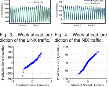
We run this week-ahead prediction on all 6 IXPs.

Figures 3 and 4 show the week-ahead (T = 7 days)

prediction result of LINX and NIX traffic for an exam-ple. We can observe that simple week-ahead prediction based on the most recent history is fairly accurate. Figures 5 and 6 show the Q-Q plots of the prediction

2. Some large IXPs, such as Deutscher IX, Amsterdam IX, and JPNAP only publish daily and/or yearly traffic stats that are too coarse to analyze. Week 1 Week 2 400 600 800 1000 1200 1400 Demand (Gbps) Original data Predicted

Fig. 3. Week-ahead pre-diction of the LINX traffic.

Week 1 Week 2 0 50 100 150 200 250 300 Demand (Gbps) Original data Predicted

Fig. 4. Week-ahead pre-diction of the NIX traffic.

−5 0 5 −300 −200 −100 0 100 200 300

Standard Normal Quantiles

Prediction Error Quantiles

Fig. 5. Q-Q plot of week-ahead prediction error on the LINX trace.

−5 0 5 −100 −50 0 50 100

Standard Normal Quantiles

Prediction Error Quantiles

Fig. 6. Q-Q plot of week-ahead prediction error on the NIX trace.

errors. They lie closely on a linear line, suggesting that

the error term✏behaves much like a Gaussian random

variable.

The error mean µand standard deviation✓ for the

week-ahead prediction on all 6 IXPs are shown in Table 1. The mean is close to zero and the standard deviation is small compared to the predicted data. Since the demand series can be accurately predicted with a small error, the 95-percentile demand can be readily calculated with the same error statistics. This validates our demand model.

Note that although the IXP data contains both elastic and inelastic traffic, essentially our demand model is based upon the observation that demand of a tier-1 ISP is highly predictable due to multiplexing, which is valid for both traffic types. We use the 95-percentile traffic from the IXP data to represent the aggregated regular transit demand_d¯_(¯_p₎_{at the regular price}_p_¯_{. We} adjust 2 [0.2,0.7]to obtain elastic traffic out of the aggregated, where denotes the relative proportion of

elastic traffic.µand✓ then scales linearly with .

The validation result also suggests that ✏ can be

modeled as a Gaussian random variable. Thus we let

A=µ 3✓andB=µ+3✓so that it contains more than

99% of the probability mass and results in reasonably good numerical accuracy and approximation [31]. The

(8)

aggregated regular transit demand _d¯_(¯_p₎ _throughout the evaluation. For a backbone with peak utilization of 50%, the underutilized capacity equals_d¯_(¯_p_{). 50%–110%} of this underutilized capacity is thus safe to be used for spot transit. We believe such setting represents a typical operating environment of spot transit. One can readily verify thatB < C holds as assumed in Sec. 3.3.

Note that we have used the simplest prediction algorithm, and the result is therefore only a lower bound. With more complex algorithms one can obtain more accurate prediction for a longer time window [30], which is beyond the focus of this paper. The prediction techniques and the line of reasoning apply to both elastic and inelastic traffic. We emphasize that our demand uncertainty model is dependent only on the observation that demand at a tier-1 ISP is highly predictable.

5.3 Obtaining cost and demand parameters from data

After validating the model, the next key step is to obtain cost and demand parameters in our model. Our analysis in Sec. 4 is applicable to general demand func-tions. In the evaluation we use two common demand functions, iso-elastic and linear demand as in Sec. 3.2.2. To derive model parameters for them, we use the Q2 2011 median GigE transit price in New York, London, and Hong Kong published in [37] as the regular transit

pricep¯in America, Europe, and Asia. Table 2 lists the

price data.

First, to obtain the cost of regular transit r¯, since

now we know the regular transit demand _d¯_(¯_p₎ _and

¯

p, assuming ISPs are rational and profit-maximizing,

from (22) we can obtain ¯ r= ¯p ✓ 1 1 ¯ ↵ ◆ (18) for iso-elastic demand with (4), and

¯

r= ¯p d¯(¯p)

¯

↵ (19)

for linear demand with (5). Studies have shown that the more elastic residential Internet traffic has an elas-ticity of around 2.7 for cable and DSL [8]. We thus

assume the demand elasticity ↵¯= 2 in (18) for

aggre-gated traffic, i.e. d¯r= 0.5¯p. Sincer¯is invariant across

two demand models, we can substitute r¯into (19) to

obtain ↵¯ for linear demand in different continents.

To obtain demand parameters, we first multiply 2

[0.2,0.7]tod¯(¯p) to calculate the elastic traffic demand

at the regular price d(¯p) from the IXP dataset. Then

from (4) and (5) we know that as long as the demand

sensitivity parameter ↵ is known we can obtain the

base demand

v=d(¯p)·p¯↵ ₍₂₀₎ for iso-elastic demand and

v=d(¯p) +↵¯p (21)

Location Pricep¯($USD/Mbps)

London 7.5

New York 7

Hong Kong 22

TABLE 2

The regular transit prices in major Internet exchange locations [37].

for linear demand. The entire elastic demand curve

d(p)can then be obtained. We use a range of values

for >1to control the relative elasticity of spot transit versus regular transit, in order to evaluate the effect of elasticity on the benefits of spot transit. For iso-elastic

demand,↵ corresponds directly to elasticity, and ↵=

¯

↵ so that spot transit is more sensitive. For linear

demand, since↵ also affects the demand magnitude,

we have to first scale it down by , i.e.↵= · ↵.¯

We stress that the purpose of evaluation is to verify the analysis in Sec. 4 and gain insights on the potential of spot transit in a realistic setting. We do not claim the numerical accuracy of the results obtained here for tier-1 ISPs. The exact pricing and monetary benefits heavily depend on various factors and can only be calculated on a case-by-case basis.

5.4 Overall benefits

First and foremost, we evaluate the overall benefits of spot transit with typical parameter setting. For both

demand models, we set = 1.25, r = 0.5¯r, and

m= ¯p so that elastic traffic, i.e. spot transit demand,

is 1.25 times more sensitive than regular transit, cost is half of the regular cost, and overflow penalty is equal to regular price. = [0.2,0.7], and the capacity C= (0.4+ ) ¯d(¯p). For a backbone with peak utilization

of 50%, the underutilized capacity equals _d¯_(¯_p_). 50%-110% of this underutilized capacity is thus safe to be used for spot transit. We believe such setting repre-sents a typical operating environment of spot transit. Figures 7-16 show the evaluation results of all 6 IXPs for both demand models.

Figures 7 and 10 plot the normalized spot transit price p⇤

¯

p for both demand models. Observe that spot

transit is offered at a discount, ranging from more than 30% to 15%. This demonstrates the price advantage of spot transit. Price increases with , suggesting that as relative proportion of elastic traffic increases, demand overflow probability increases since cost, penalty, and

elasticity does not change with here. Figures 8 and

11 show the profit improvement of spot transit. We can see that spot transit significantly improves tier-1 ISP’s profit, by 80%-130% with iso-elastic demand, and by 63%-65% with linear demand. Same observation can be made in terms of consumer surplus as shown in Figures 14 and 16. Spot transit improves surplus by 10%-40% with iso-elastic demand, and by 120%-200% with linear demand. Since price increases with , the improvement decreases as a result.

(9)

0.2 0.3 0.4 0.5 0.6 0.7 0.6

0.7 0.8 0.9

Proportion of elastic traffic

Normalized spot price

LINX MSKIX NIX NYIIX ESPANIX HKIX

Fig. 7. Optimal spot price with iso-elastic demand. 0.2 0.3 0.4 0.5 0.6 0.7 0.7 0.9 1.1 1.3 1.5

Profit improvement LINX MSKIX NIX NYIIX ESPANIX HKIX

Fig. 8. Profit improvement with iso-elastic demand. 0.2 0.3 0.4 0.5 0.6 0.7 0.2 0.4 0.6 0.8

Surplus improvement LINX MSKIX NIX NYIIX ESPANIX HKIX

Fig. 9. Surplus improvement with iso-elastic demand. 0.2 0.3 0.4 0.5 0.6 0.7 0.82 0.84 0.86 0.88 0.9

Fig. 10. Optimal spot price with linear demand. 0.2 0.3 0.4 0.5 0.6 0.7 0.63 0.64 0.65 0.66

Fig. 11. Profit improvement with lin-ear demand. 0.2 0.3 0.4 0.5 0.6 0.7 1 1.2 1.4 1.6 1.8 2

Fig. 12. Surplus improvement with linear demand. 0.2 0.3 0.4 0.5 0.6 0.7 0 0.5 1 1.5 2 2.5

$USD (Million) LINX MSKIX NIX NYIIX ESPANIX HKIX

Fig. 13. Profit gain of spot transit with iso-elastic de-mand. 0.2 0.3 0.4 0.5 0.6 0.7 0 2 4 6

$USD (Million)

Fig. 14. Surplus gain of spot transit with iso-elastic demand. 0.2 0.3 0.4 0.5 0.6 0.7 0 0.5 1 1.5 2

$USD (Million) LINX MSKIX NIX NYIIX ESPANIX HKIX

Fig. 15. Profit gain of spot transit with linear demand.

0.2 0.3 0.4 0.5 0.6 0.7 0 0.5 1 1.5 2 2.5

$USD (Million)

Fig. 16. Surplus gain of spot transit with linear de-mand.

One may wonder at this point, what is the exact dollar amount of spot transit’s benefits? Figures 13 and 16 plot the absolute profit and surplus gain for iso-elastic demand, and Figures 14 and 15 plot the abso-lute gains for linear demand, respectively. The profit gain stands more than $1 million for large IXPs like LINX, and in the order of hundreds of thousands of

dollars for smaller ones like NIX, NYIIX and ESPANIX for both models. The absolute surplus gain depends more on the shape of demand curve, and is more salient with iso-elastic demand that allows price to go to infinity. Again the gain is in the order of million dollars for large IXPs, and hundreds of thousands of dollars for smaller ones. Thus, our evaluation not only confirms the qualitative analysis in Sec. 4.2, but also quantitatively shows that spot transit offers significant financial incentives with more than $1 million dollars of gains possible (monthly) for both tier-1 ISPs and transit customers, depending on the size of the ISP.

Another interesting observation from the results is that, the smallest IXP, HKIX, enjoys more dramatic performance improvement than others despite its rel-atively small scale, especially in terms of consumer surplus. The reason is that the regular transit price in Asia and other more remote areas of Internet is much higher than other regions, resulting in a much larger profit margin in $/Mbps for tier-1 ISPs. Thus, with the same price discount, its profit and surplus gains are more profound than bigger IXPs in major cities of Europe and America. This illustrates that spot transit is potentially more attractive in “remote” regions of Internet where regular transit is much more expensive.

5.5 Pricing analysis

Now we the effect of various parameters on spot tran-sit pricing. We choose to present results with iso-elastic demand since both models lead to similar conclusions.

(10)

0.1 0.3 0.5 0.7 0.9 0.65

0.7 0.75

Relative spot transit cost

Fig. 17. The effect ofron spot price

with iso-elastic demand.

0.5 0.7 0.9 1.1 1.3 1.5 0.62 0.63 0.64 0.65 0.66 0.67

Relative overflow penalty

Fig. 18. The effect ofmon spot price

with iso-elastic demand.

1.2 1.4 1.6 1.8 2 0.6

0.65 0.7 0.75

Relative elasticity (gamma)

Fig. 19. The effect of on spot price with iso-elastic demand.

Figures 17-19 show how spot transit price is affected by costr, penaltym, and elasticity↵, respectively. We

vary the relative cost r/r¯ between 0.1 and 0.9 with

m = ¯p and = 1.25, relative penalty m/p¯ between

0.5 and 1.5 with r = 0.5¯r and = 1.25, and relative

elasticity between 1.1 and 2 with r = 0.5¯r and

m = ¯p. Other parameter settings remain the same as

in the previous section. We observe that spot price increases with all of the three factors, as expected from Theorem 1. Price is less sensitive to penalty

m compared to cost and elasticity, since penalty is

only imposed on the overflown portion of demand.

Also from Figure 17 we can see that when r 0.4¯r,

¯

r r  0.6¯r = 0.3¯p < 0.5m(1 ₂_⇤₁1_.₂₅) = 0.3¯p, spot

transit price is still offered at more than 15% discount. This confirms our discussion of Theorem 2 in Sec. 4.1 that even when the conditionr¯r 0.5m(1 (p⇤₎ 1₎ is not satisfied, i.e. when the cost difference is not large, spot transit can still be much cheaper than regular transit, and improves the overall efficiency of the market as proved in Theorem 3.

5.6 Sensitivity analysis

We have studied how costr, penaltym, and elasticity

↵affect spot transit pricing. In this section, we analyze how these model parameters affect the profit and surplus improvement of spot transit.

First we vary r and m individually as we did in

the previous section, and plot the profit and surplus improvement with iso-elastic demand in Figures

20-23. Observe that as cost r and penalty m increase,

both profit and surplus drop which is intuitive to understand. Spot transit is able to provide positive improvement even whenr= 0.9¯rorm= 1.5¯p. Results

of linear demand are similar and not presented.

We then vary elasticity↵ by varying between 1.1

and 2. Figures 24-25 show the corresponding profit and surplus improvement. We can see that although a

larger↵ increases spot transit prices, it also increases

the profit and surplus gains at the same time, which is in sharp contrary to the results of cost and penalty.

The reason for the discrepancy is that increasing ↵

does not change cost and penalty of spot transit, and as a result the profit margin is actually increased due

0.1 0.3 0.5 0.7 0.9 0

1 2 3

Fig. 20. Profit

improve-ment vs. r with iso-elastic

demand. 0.1 0.3 0.5 0.7 0.9 0.2 0.3 0.4 0.5 0.6 0.7

Fig. 21. Surplus

improve-ment vs. r with iso-elastic

demand. 0.5 0.7 0.9 1.1 1.3 1.5 1.3 1.35 1.4 1.45

Fig. 22. Profit

improve-ment vs.mwith iso-elastic

demand. 0.5 0.7 0.9 1.1 1.3 1.5 0.3 0.4 0.5 0.6

Fig. 23. Surplus

improve-ment vs.mwith iso-elastic

demand.

to the price increase. From the numerical result we

also observe that demand atp⇤ also increases despite

the price increase because the elasticity now is larger. The overall effect of increased elasticity therefore is positive, in spite of slightly increased revenue loss due to demand overflow either.

1.2 1.4 1.6 1.8 2 1

1.5 2 2.5

Fig. 24. Profit

improve-ment vs. with iso-elastic

demand. 1.2 1.4 1.6 1.8 2 0.2 0.4 0.6 0.8 1

Fig. 25. Surplus

improve-ment vs. with iso-elastic

demand.

Finally, we study aworst-casescenario, where all the

(11)

the worst operating environment with high cost, high penalty, and low elasticity for spot transit. Specifically, we let r = 0.9¯r, m = 1.5¯p, and = 1.1, and plot

the spot transit price, profit and surplus improvement

with varying in Figures 26-31. In other words, these

figures represent the minimum improvement over a

range of parameter values.

0.2 0.3 0.4 0.5 0.6 0.7 0.8 0.85 0.9 0.95 1

Fig. 26. Worst-case price with iso-elastic demand.

0.2 0.3 0.4 0.5 0.6 0.7 0.9

0.92 0.94 0.96

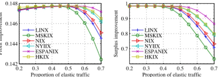
Fig. 27. Worst-case price with linear demand. We can see that with the worst combination of parameters, spot transit is still slightly cheaper than regular transit for both demand models. The profit improvement stands above 10%, and the surplus im-provement is 5% with iso-elastic demand and more than 60% with linear demand. The results clear demonstrates that the advantage of spot transit is robust against a wide range of parameter values, and spot transit can be expected to provide significant gains in a typical operating environment.

0.2 0.3 0.4 0.5 0.6 0.7 0.125 0.13 0.135 0.14 0.145 0.15

Profit improvement LINX MSKIX NIX NYIIX ESPANIX HKIX Fig. 28. Worst-case

profit improvement with iso-elastic demand. 0.2 0.3 0.4 0.5 0.6 0.7 0 0.05 0.1 0.15 0.2 0.25

Fig. 29. Worst-case sur-plus improvement with iso-elastic demand. 0.2 0.3 0.4 0.5 0.6 0.7 0.142 0.144 0.146 0.148

Fig. 30. Worst-case profit improvement with linear demand. 0.2 0.3 0.4 0.5 0.6 0.7 0.7 0.8 0.9 1

Fig. 31. Worst-case sur-plus improvement with lin-ear demand.

6 D

ISCUSSION OF

F

EASIBILITY

We have compellingly demonstrated, through both theoretical analysis and empirical evaluation based

on real-world traffic and price data, that spot transit provides significant financial benefits to tier-1 ISPs and transit customers. However, profitability alone does not guarantee the feasibility of spot transit. In this section, we examine some practical aspects that we believe are important to the establishment of such a new transit settlement market.

6.1 Market infrastructure

In the spot transit market, customers can purchase and utilize spot transit on-demand from tier-1 ISPs. This requires a physically connected infrastructure amongst all customers and the ISP. We believe this seemingly daunting task has, to a large extent, been solved by the proliferation of network exchange fa-cilities, such as Internet Exchange Points (IXP) and Network Access Points (NAP), across the world. They host hundreds of ISPs each already, including tier-1 ISPs [4]. Though IXPs carry mostly peering traffic for now, the infrastructure can certainly be utilized to support spot transit with little additional cost. Such a public infrastructure enables tier-1 ISPs to support any customers present in the IXP, and customers to flexibly switch between spot transit providers. By supporting spot transit IXPs also diversify and expand its business line.

In case the tier-1 ISP or the transit customer is not present in an IXP, it is highly likely that a private link exists between the two for carrying regular transit. Spot transit can then be provided over the existing private link. Even in the extremely rare case that a new link has to be set up, such a one-time cost is expected to be rather insignificant compared to the long-term benefits of spot transit.

6.2 Inter-domain routing, service differentiation, and billing

The introduction of spot transit traffic does not pose technical challenges or complications for inter-domain routing of BGP (Border Gateway Protocol). Though it shares the same network backbone with regular transit traffic, spot transit traffic can be easily identified and managed by a designated AS (Autonomous System) number acquired by the tier-1 ISP. The ISP advertises routes with the designated AS number when it sup-ports spot transit, and stops doing so when it does not wish to carry spot transit due to say insufficient capacity or other considerations.

To make sure spot transit traffic does not negatively impact regular traffic, ISPs may wish to impose service differentiation, e.g. bandwidth limit. In fact ISPs have been practicing service differentiation for many years and there is little additional difficulty in managing spot transit traffic. For example, an ISP can rely on differentiated services (DiffServ) commonly used to provide to provide different QoS. It recognizes spot transit traffic by the designated AS number, and clas-sify it by setting the DSCP (differentiated services code

(12)

point) bits in the IP header of packets to have a lower priority than regular transit traffic. The ISP then can compute and limit the total bandwidth used by spot transit packets. Or it may use priority queueing based on the DSCP bits so that packets of spot transit traffic will only be forwarded by the routers when there is no packet from regular transit traffic in the egress port.

Billing is also straightforward by tracking traffic destined to the designated AS number. No contract is required and only the used amount of bandwidth is billed based on 95-th percentile billing or any other suitable method. The spot transit bill can easily be combined with the regular transit bill if the customer uses both from the same tier-1 ISP.

6.3 Market cannibalization

One may be concerned that the tier-1 ISP’s regular transit business would be negatively impacted by of-fering spot transit customers, resulting in the so-called market cannibalization [2]. We have already shown that, the spot transit profit is significantly larger than the profit collected from serving the elastic traffic with regular transit due to an increase of demand as a result of price reduction. The demand increase does not necessarily translate to a decrease of regular transit demand. In fact we do not expect spot transit to be suitable for the relatively inelastic traffic which finds regular transit with SLAs more reliable.

The demand increase with spot transit can be ex-plained by at least two factors: competition with peer-ing and transit resellpeer-ing. The low price and on-demand feature of spot transit can make it more appealing than peering or paid peering, considering the performance benefits and network reachability provided by the tier-1 backbone. An ISP that relies mostly on (paid) peering for cost reasons can utilize spot transit for a portion of its elastic traffic with much better reachability. Further, small ISPs usually find it difficult to purchase transit directly from tier-1 ISPs due to the minimum com-mitted data rate requirement. They purchase transit from medium size ISPs that buy transit at bulk and resell to these small customers. With spot transit, tier-1 ISPs are able to collect additional profits from small ISPs by bypassing the transit resellers in the middle.

In all, we expect that spot transit compliments rather

than cannibalizes the traditional transit business of a tier-1 ISP.

7 R

ELATED

W

ORK

An extensive literature exists on the Internet transit market in both networking and economics. Two as-pects are particularly related to our work: optimal pric-ing design, and novel market approaches for Internet transit.

Internet broadband access pricing generally is de-signed and computed to optimize revenue, social wel-fare, or performance. [29] argues that the predominant

flat-rate pricing structure for selling retail Internet access encourages waste and is incompatible with service differentiation. [17], [32] study the benefits of usage-based pricing and argue that, with price differ-entiation, one can use resources more efficiently. [10], [28] study Paris Metro Pricing in which service dif-ferentiation and congestion control are autonomously achieved by charging different prices for different service tiers that share the same infrastructure. Time is

another dimension to unbundle connectivity. Handeet

al.[14] characterize the economic loss due to the ISP’s

inability or unwillingness to price broadband access

based on time of day. Jianget al.[16] study the optimal

time-dependent prices for an ISP selling broadband ac-cess based on solving optimization offline with traffic estimates.

Our work is different in that we study pricing of spot transit, a new market for Internet transit. [21] proposes a Shapley value based cooperative settlement between content, transit, and eyeball ISPs. The focus is on performance and optimality of the Internet ecosys-tem with selfish ISPs through fair and efficient profit sharing. [38] proposes a clean-slate market structure and routing protocol for exchange of Internet paths. [9], [35], [39] are more related to our work. [39] stud-ies tiered pricing based on packet destinations and routing costs for selling Internet transit. It is shown that a few tiers is enough to capture the optimal profit gain for a tier-1 ISP. From the customer’s perspective, [35] proposes to use Tuangou (group buying), and [9] innovates T4P (transit for peering) that provides partial transit to peering partners, to reduce transit costs.

Spot transit is orthogonal to these novel settlement schemes, and compliments them in that tiered pricing, Tuangou, and T4P can be readily applied in spot tran-sit market just like they are used in the regular trantran-sit market. The benefits of spot transit, as mentioned, depend on the very characteristics of elastic traffic instead of the specifics of settlement details. We use a simple model derived from [23], [31] where demand randomness is modeled additively. The technical dis-tinction is clear: we use a general demand function and analyze the profit and surplus improvement, while [23], [31] only study pricing based on a linear demand function.

8 C

ONCLUDING

R

EMARKS

In this paper, we advocate to create a spot transit

market, where under-utilized backbone capacity is offered at discounted to serve elastic traffic, and transit customers can purchase transit on-demand. We sys-tematically studied the pricing and economical bene-fits of spot transit. Through both theoretical analysis and empirical evaluation with real-world price and traffic data, we demonstrated that significant profit and surplus improvement can be generally expected from the spot transit market. The gains are also robust

(13)

for a wide range of parameter settings. Given the potential economical benefits, we believe spot transit will encourage many entities to engage in this new market.

We conclude the paper by pointing out some in-teresting open problems with the introduction of spot transit. For example, how can the tier-1 ISP use smart traffic engineering algorithms to provide better perfor-mance isolation between the regular and spot transit traffic? How do we quantify the effect of spot transit on novel settlement schemes such as paid peering? How would it change the Internet AS level topology, and the entire ecosystem? Lastly, it is also interesting to study other pricing strategies for the spot market, such as derivative following, regret-based pricing, etc. from microeconomics, and compare their effectiveness.

R

EFERENCES

[1] http://gigaom.com/2010/12/07/a-play-by-play-on-the-comcast-and-level-3-spat/.

[2] Market cannibalization. http://www.investopedia.com/ terms/m/marketcannibilization.asp#axzz1t6LbAnss.

[3] IXP traffic dataset. http://www.cs.cityu.edu.hk/⇠hxu/share/ IXPdata.zip, 2013.

[4] List of internet exchange points by size. http://en.wikipedia. org/wiki/List of Internet exchange points by size, 2013. [5] Tobi Oetiker’s MRTG—-The multi router traffic grapher. http:

//oss.oetiker.ch/mrtg/, 2013.

[6] K. J. Arrow and A. C. Enthoven. Quasi-concave programming.

Econometrica, 29(4):779–800, October 1961.

[7] C. M. Bishop. Pattern Recognition and Machine Learning. Springer, 2006.

[8] M. Cardona, A. Schwarz, B. B. Yurtoglu, and C. Zulehner. De-mand estimation and market definition for broadband Internet services. Journal of Regulatory Economics, 35(1):70–95, July 2007. [9] I. Castro and S. Gorinsky. T4P: Hybrid interconnection for cost

reduction. InProc. NetEcon, 2012.

[10] C.-K. Chau, Q. Wang, and D.-M. Chiu. On the viability of Paris Metro Pricing for communication and service networks. InProc. IEEE INFOCOM, 2010.

[11] Y. Chen, S. Jain, V. K. Adhikari, Z.-L. Zhang, and K. Xu. A first look at inter-data center traffic characteristics via yahoo! datasets. InProc. IEEE INFOCOM, 2011.

[12] Cisco Systems. Cisco visual networking index: Forecast and methodology, 2010-2015. A Cisco White Paper, June 2011. [13] C. Fraleigh, S. Moon, B. Lyles, C. Cotton, M. Khan, D. Moll,

R. Rockell, T. Seely, and S. Diot. Packet-level traffic measure-ments from the Sprint IP backbone. IEEE Netw., 17(6):6–16, November 2003.

[14] P. Hande, M. Chiang, R. Calderbank, and J. Zhang. Pricing under constraints in access networks: Revenue maximization and congestion management. InProc. IEEE INFOCOM, 2010. [15] Hong Kong Internet Exchange. http://www.hkix.net/hkix/

stat/aggt/hkix-aggregate.html, March 2012.

[16] C. Joe-Wong, S. Ha, and M. Chiang. Time-dependent broad-band pricing: Feasibility and benefits. In Proc. IEEE ICDCS, 2011.

[17] G. Kesidis, A. Das, and G. de Veciana. On flat-rate and usage-based pricing for tiered commodity Internet services. In

Proc. CISS, 2008.

[18] C. Labovitz, S. Iekel-Johnson, D. McPherson, J. Oberheide, and F. Jahanian. Internet inter-domain traffic. InProc. ACM SIGCOMM, 2010.

[19] N. Laoutaris, M. Sirivianos, X. Yang, and P. Rodriguez. Inter-datacenter bulk transfers with netstitcher. InProc. ACM SIG-COMM, 2011.

[20] London Internet Exchange Ltd. https://stats.linx.net/cgi-pub/ exchange?log=combined.bits, March 2012.

[21] R. T. Ma, D. Chiu, J. C. Lui, V. Mistra, and D. Rubenstein. On cooperative settlement between content, transit and eyeball Internet service providers. InProc. ACM CoNEXT, 2008.

[22] A. Mas-Colell, M. D. Whinston, and J. R. Green.Microeconomic Theory. Oxford University Press, 1995.

[23] E. S. Mills. Uncertainty and price theory. Quart. J. Econom., 73(1):116–130, February 1959.

[24] J. Mo and J. Walrand. Fair end-to-end window-based con-gestion control. IEEE/ACM Trans. Netw., 8(5):556–567, October 2000.

[25] Moscow Internet Exchange. http://www.msk-ix.ru/eng/ traffic.html, March 2012.

[26] Neutral Internet eXchange. http://www.nix.cz/index.php?lg= en&wid=54, March 2012.

[27] New York International Internet Exchange. http://www.nyiix. net/mrtg/sum.html, March 2012.

[28] A. Odlyzko. Paris Metro Pricing for the Internet. InProc. ACM EC, 1999.

[29] A. Odlyzko. Should flat-rate Internet pricing continue? IEEE IT Prof., 2:48–51, 2000.

[30] K. Papagiannaki, N. Taft, Z.-L. Zhang, and C. Diot. Long-term forecasting of Internet backbone traffic: Observations and initial models. InProc. IEEE INFOCOM, 2003.

[31] N. C. Petruzzi and M. Dada. Pricing and the newsvendor problem: A review with extensions. Oper. Res., 47(2):183–194, February 1999.

[32] S. Shakkottai, R. Srikant, A. Ozdaglar, and D. Acemoglu. The price of simplicity.IEEE J. Sel. Areas Commun., 26(7):1269–1276, September 2008.

[33] S. Shenker. Fundamental design issues for the future Internet.

IEEE J. Sel. Areas Commun., 13(7):1176–1188, September 1995. [34] Spain Internet Exchange. http://mrtg.espanix.net/espanix/

espanix.html, March 2012.

[35] R. Stanojevic, I. Castro, and S. Gorinsky. CIPT: Using Tuangou to reduce IP transit costs. InProc. ACM CoNEXT, 2011. [36] TeleGeography Research. Global Internet geography executive

summary. http://bpastudio.csudh.edu/fac/lpress/471/hout/ telegeographygig execsumm.pdf, 2008.

[37] TeleGeography Research. Global Internet geography executive summary. http://www.telegeography.com/research-services/ global-internet-geography/index.html, 2011.

[38] V. Valancius, N. Feamster, R. Johari, and V. Vazirani. MINT: A market for INternet transit. InProc. ACM CoNEXT, 2008. [39] V. Valancius, C. Lumezanu, N. Feamster, R. Johari, and V. V.

Vazirani. How many tiers? Pricing in the Internet transit market. InProc. ACM SIGCOMM, 2011.

[40] D. Xu and X. Liu. Geographic trough filling for Internet datacenters. InProc. IEEE INFOCOM, 2012.

Hong Xureceived the B.E. degree from the Department of Information Engineering, The Chinese University of Hong Kong, in 2007, and the M.A.Sc. and Ph.D. degrees from the Department of Electrical and Computer Engineering, University of Toronto. He joined the Department of Computer Science, City University of Hong Kong in August 2013, where he is currently an assistant professor. His research interests include data center networking, cloud computing, network eco-nomics, and wireless networking. He is a member of ACM and IEEE.

(14)

Baochun Lireceived the B.E. degree from the Department of Computer Science and Technology, Tsinghua University, China, in 1995 and the M.S. and Ph.D. degrees from the Department of Computer Science, Univer-sity of Illinois at Urbana-Champaign, Urbana, in 1997 and 2000.

Since 2000, he has been with the Depart-ment of Electrical and Computer Engineer-ing at the University of Toronto, where he is currently a Professor. He holds the Nortel Networks Junior Chair in Network Architecture and Services from October 2003 to June 2005, and the Bell Canada Endowed Chair in Computer Engineering since August 2005. His research interests in-clude large-scale distributed systems, cloud computing, peer-to-peer networks, applications of network coding, and wireless networks.

Dr. Li was the recipient of the IEEE Communications Society Leonard G. Abraham Award in the Field of Communications Systems in 2000. In 2009, he was a recipient of the Multimedia Communica-tions Best Paper Award from the IEEE CommunicaCommunica-tions Society, and a recipient of the University of Toronto McLean Award. He is a senior member of IEEE and IEEE Computer Society and a member of ACM.