Nested separatrices in simple shear flows: the effect of localized disturbances on stagnation lines

promoting access to White Rose research papers

White Rose Research Online

Universities of Leeds, Sheffield and York

http://eprints.whiterose.ac.uk/

This is an author produced version of a paper published in Physics of Fluids.

White Rose Research Online URL for this paper: http://eprints.whiterose.ac.uk/3653/

Published paper

Wilson, M. C. T., Gaskell, P. H. & Savage, M. D. (2005) Nested separatrices in simple shear flows: the effect of localized disturbances on stagnation lines,

Physics of Fluids, Volume 17 (9), 093601.

This is an author-prepared final version of a paper appearing in Physics of Fluids, 17, 093601 (2005)

Nested separatrices in simple shear flows: the effect

of localized disturbances on stagnation lines

M. C. T. Wilson and P. H. Gaskell

School of Mechanical Engineering, University of Leeds, Leeds LS2 9JT, UK

M. D. Savage

Department of Physics and Astronomy, University of Leeds, Leeds LS2 9JT, UK

Abstract: _{The effects of localized two-dimensional disturbances on the structure of}

I

Introduction

Stagnation points (or ‘critical points’) are essential features of many non-trivial flows across a broad Reynolds number spectrum. In addition to appearances in jets and wakes1_{, for example, they often arise in laminar flows such as mixing, stirring and} coating flows2−4_{, and of course in cavity flows}5,6_{. In such cases, global streamline} pat-terns can often be deduced from an analysis of the flow behaviour local to stagnation points without having to find a complete solution to the problem. This approach has long been familiar in dynamical systems theory, the techniques and vocabulary of which have consequently been brought to bear upon the general study of flow structures7−10_.

On the other hand, stagnation lines — streamlines upon which fluid velocity vanishes — arise only in idealised flows such as shear flow between infinite parallel plates, or Couette flow in an infinitely long concentric circular annulus. However, there are certain flows in geometries similar to those just mentioned where one would expect to see a feature similar to a stagnation line. The archetypal example is shear flow past a stationary or rotating cylinder, which has received much attention in the literature11−17 _{due to its relevance to the study of particles in suspension — the case} of a freely rotating cylinder naturally being of particular interest. So the question is ‘what happens to the stagnation line when a cylinder is placed upon it?’

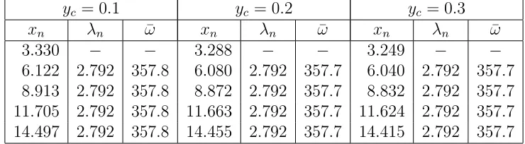
Early work on shear flow past a cylinder11−15 _{considered only the case of unbounded} shear flow, in which the streamfunction approaches that of simple shear as the distance from the cylinder increases. Jeffrey and Sherwood15 _{summarized the resulting flow} structures, which differ according to the rotational speed of the cylinder. Some of the structures are reproduced in Fig. 1. In the stationary cylinder case, both the Stokes solution and matched asymptotic solutions for small Reynolds number (Re) feature a region of ‘blocked’ flow where fluid approaching the obstacle is turned around and sent in the opposite direction. Though the vertical velocity component in this region diminishes very rapidly with distance from the cylinder, the width of the region increases logarithmically13_{. Thus the stagnation line disappears completely.}

The present work focuses on the fate of the stagnation line in the case when the flow is confined by the presence of parallel plates. Though confinement effects in the shear flow past a cylinder have been considered before16,17_{, attention has been concentrated} on the resulting rotation rates of freely-suspended cylinders. The structure of the flow along the stagnation line has not been considered.

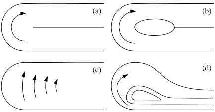
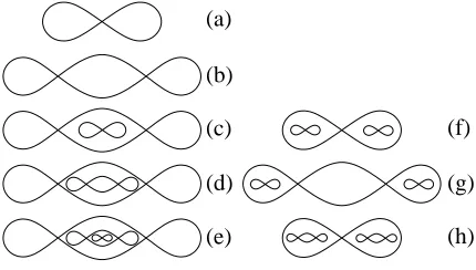
In addition to the above motivation, interest in this problem has also been aroused from another source, namely a discussion at the end of a paper by Brøns and Hartnack10 who presented a thorough theoretical analysis of two-dimensional streamline topolo-gies close to critical points arising away from boundaries. Their approach involved the expansion of the velocity field about degenerate critical points and the subsequent manipulation of the expansions into canonical form so that bifurcations in the flow structure could be described in detail. As an example of how their theory can be applied, Brøns and Hartnack cited a study of Stokes flow in a (horizontal) half-filled annular cavity by Gaskellet al.19, who had observed from numerical calculations that as the gap between their cylinders decreased, a growing chain of stagnation points was generated. The structure of the flow is shown in Fig. 3(a–e). It was recognized by Gaskellet al. that the same stagnation points could in general form other struc-tures, e.g. Fig. 3(f–h), and this was confirmed by the theoretical analysis of Brøns and Hartnack, which predicted that since the problem had two bifurcation parameters (the cylinder radius and speed ratios), structures (f), (g) and (h) should generally be realizable. It was suggested10 _{that the absence of the alternative structures in the} annulus is perhaps due to the assumption that the free surfaces are radial lines, giv-ing an exactly half-filled annulus, and that changgiv-ing the fill fraction as an additional parameter might produce the missing patterns.

Here it is argued from a more general perspective that the position and shape of the free surfaces (which are effectively the ‘end’ boundaries of the long, thin domain) are not important in determining which of the alternative bifurcation sequences is observed. Rather, it is the uniformity of the narrow gap between the coaxial cylinder surfaces which dictates that only the sequence of structures seen by Gaskellet al.19

is possible.

II

Flow between infinite parallel plates

A

Stationary plates

As part of his paper on eddies near a sharp corner, Moffatt21 _{examined the flow} between infinite stationary parallel plates due to an arbitrary disturbance, for example a rotating cylinder — see Fig. 4(a). That a sequence of eddies should exist in this geometry was indicated by considering it as a limiting case of the flow in a corner between two plates, where the angle between the plates vanishes while keeping fixed a point on each plate. Rather than take this limit formally, however, Moffatt solved the biharmonic equation more easily by postulating a streamfunction of the form

ψ ∼f(y)e−k|x|_{. The even function f(y) was found to bef(y) =Acosky+Bysinky,}

and imposition of the no-slip boundary conditions on y =±a produced an equation fork,

2ka+ sin 2ka= 0, (1)

and the streamfunction

ψ =A(asinkacosky−ysinkycoska)e−kx (x >0), (2)

where the parameter A is dictated by the strength of the disturbance, and is taken to be positive. Equation (1) has no real solution, and the complex solution with smallest positive real part is21 _{k = p+qi ≈ (4.21 + 2.26i)/2a. The flow described} by (2) consists of a sequence of equal-size eddies rotating alternately in the clockwise and anticlockwise senses, as sketched in Fig. 4(a). Following Moffatt, local extrema in the vertical velocity component, v, can be used as a measure of the ‘strength’ of each eddy in order to define a damping factor in terms of the relative strengths of adjacent eddies. To this end, the vertical velocity along the liney= 0 is given by

v(x,0) =Aaγe−pxsin(qx+δ), (3)

where γ and δ are functions of pa and qa and are approximately 3.898 and 1.525 respectively. The local extrema obviously occur when qxn+δ = (n+ 1₂)π, giving a

damping factor of

¯ ω= vn

vn+1

= e

−pxn

e−pxn+1 =e

pπ/q _{≈353. (4)}

The wavelength of the eddy pattern, i.e. the distance between the centres of consec-utive co-rotating eddies, is given by 2π/q ≈5.56a. A quantity of interest later is the separation between the centres of adjacent eddies, which is simply half the above, namely

λ≈2.78a. (5)

B

Translating plates

In order to observe the effects of a distant arbitrary disturbance on a stagnation-line flow, one can simply superpose Moffatt’s streamfunction and that corresponding to the flow of interest. Consider first an antisymmetric Couette flow between plates located aty=±atranslating in-plane with speeds±U. For simplicity, the problem is non-dimensionalized by scaling all lengths by a and all velocities by U. The Couette flow velocity components are then uc = y and vc ≡ 0. Let um and vm be the

dimensionless velocity components corresponding to (2); the combined flow is then given by (u, v) = (um+uc, vm +vc). The superposition is sketched in Fig. 4(b). It

is clear that in this case the stagnation points at the centres of the eddies are also present in the combined flow, but the points are no longer all elliptic: the stagnation points corresponding to the anticlockwise eddies (i.e. those opposing the sense of the plate motion) become hyperbolic (saddle points).

This is easily confirmed by examining the usual linear expansion of the velocity field about each stagnation point10_:

u v = ∂u ∂x ∂u ∂y ∂v ∂x ∂v ∂y

x−xs

y−ys

, (6)

where (xs, ys) are the coordinates of a stagnation point. If the determinant

|J|= ∂u

∂x ∂v ∂y − ∂u ∂y ∂v ∂x (7)

is positive, the stagnation point is a centre, while |J| < 0 implies a saddle point10_. Now, the expression (7) can be simplified somewhat since u = 0 everywhere along

y = 0, and so the first term vanishes. In addition, ∂v/∂x =∂vm/∂x and ∂u/∂y ≈ 1

since ∂um/∂y ≪ ∂uc/∂y = 1. Hence only ∂vm/∂x is needed to determine the type

of each stagnation point (with a positive value of ∂vm/∂xindicating a saddle). From

(3), stagnation points exist where qxn+δ =nπ, so at stagnation point n,

∂vm ∂x n

=Aγqe(δ−nπ)p/qcosnπ = (−1)nAγqe(δ−nπ)p/q. (8)

Hence for evenn(anticlockwise Moffatt eddies) the stagnation point is a saddle, while for oddn a centre remains.

Fig. 4(c) shows a sketch of the decay of the combined streamfunction along the line

y = 0, assuming that the streamfunction value corresponding to the stagnation line in the Couette flow is zero. This damped form of ψ, combined with the alternating nature of the stagnation points, implies the ‘nested separatrix’ flow structure given in Fig. 4(d), which is consistent with the numerical observations of Gaskellet al.19.

When the stagnation line of the moving-plate flow does not lie along the centreline

flow is topologically the same: the anticlockwise eddies still produce saddle points and the decay of the streamfunction gives the same nested flow structure. However, since the eddy centres no longer lie along the stagnation line, the resulting stagnation points are shifted vertically — see Fig. 4(e). The degree and direction of the shift are determined by the strength and sense of rotation of each eddy. A closer look at Fig. 4(e), to find where uc =−um, reveals that the elliptic points (•) lie between the

stagnation line and the corresponding eddy centre (+), while the hyperbolic points (×) appear on the opposite side of the stagnation line from the eddy centre. Since

um decays exponentially with x, the displacement of the stagnation points from the

stagnation line likewise decreases with x. The final schematic in Fig. 4 shows the resulting distorted flow pattern.

III

Shear flow past a cylinder

One can perhaps envisage a number of scenarios in which a shear flow featuring a stagnation line could be perturbed by two-dimensional effects. In addition to ‘active’ mechanisms such as the rotating cylinder mentioned above or moving sleeves25_{, a} flow could of course be disturbed in a variety of ‘passive’ ways such as the mere presence of a stationary obstacle, or, in the case of a Couette-Poiseuille flow with adverse pressure gradient, by a cavity, protrusion or other local non-uniformity in the stationary boundary surface. Here, attention is focused on the effect of a cylindrical obstacle in a simple shear flow between infinite parallel plates separated by a gap of 2a and moving in opposite directions with velocitiesUt>0 andUb <0. As explained

in the introduction, this problem has received much attention in the literature, but as yet the structure of the flow near the stagnation line has not been explored.

A

Numerical method

The fluid is assumed to be Newtonian, with constant density, ρ, and viscosity µ, and the problem is non-dimensionalised by scaling all lengths by a, all velocities by the speed of the lower plate, |Ub|, and pressures by µ|Ub|/a. The dimensionless speed of

the upper plate is denoted by S =Ut/|Ub| and the dimensionless shear rate produced

by the motion of the plates is then ˙γc = 1₂(S+ 1). The corresponding dimensionless

governing equations are

Reu_.∇u _{= −∇p+∇}2u_{, (9)}

∇.u _{= 0, (10)}

whereu _{= (u, v) is the fluid velocity, pis pressure, andRe=ρa|Ub|/µis the Reynolds}

number.

r, is located at (0, yc). Equations (9) and (10) are solved in this domain using a

Galerkin finite element method which has been applied successfully to many laminar flow problems26_{. The domain is tessellated by six-node triangular elements upon} which velocity and pressure are represented by biquadratic (Qj) and bilinear (Lk)

interpolation functions:

u ₌

6 X

j=1

u_{jQj, p=}

3 X

k=1

pkLk, (11)

where u_{j and pk are the nodal values. Substituting (11) into (9) and (10),}

weight-ing the latter equations by Qj and Lk respectively, and integrating the resulting

expressions over the whole domain generates a non-linear system of algebraic residual equations which is solved via Newton iteration. The boundary conditions imposed are no slip on the plates and the cylinder surface, and a ‘free boundary condition’27 on the left- and right-hand boundaries.

In addition to modelling flows in fixed domains, the finite element approach is also well-suited to free-surface problems28_{, and advantage is taken of this flexibility here.} Since the primary goal of the numerical analysis is the exploration of the flow near the stagnation line, the computational mesh is made to deform such that key nodes and element edges lie along two curves where the horizontal velocity component vanishes, i.e. whereu= 0 — see Fig. 5. This is achieved by allowing the y-coordinates of these nodes, yi, to be unknowns which are determined as part of the Newton iteration

procedure by weighting the equation u= 0 byQi and integrating along the curve to

form another residual equation. One can then easily investigate the behaviour of the vertical velocity component, and locate any stagnation points. Note that, as shown in Fig. 5, the u= 0 curves on each side of the cylinder terminate a small distance away from the cylinder on the vertical dashed lines. This is to prevent excessive element distortion near the cylinder, where the u= 0 curve deviates substantially fromy= 0 when yc 6= 0. In the region between the vertical dashed lines, the mesh is constructed

with respect to a polar origin at the centre of the cylinder.

The numerical calculations were performed using double-precision arithmetic, with a machine epsilon of 2.22×10−16_{, and the finite element equations were solved subject} to the convergence criterion that theL2 norm of the residuals be less than 10−12. The accuracy of the results presented below was confirmed by repeating the calculations using a higher resolution mesh (the meshes having 21 476 and 65 218 elements respec-tively); in all cases the differences between values calculated on the two meshes were negligible.

B

Results

sign of the chain of stagnation points expected from the superposition of Sec. II.B. Fig. 6 shows extended streamline plots for two different cylinder radii (r = 0.5 and 0.9) with yc = 0, Re = 0 and ˙γc = 1. Though it is not possible to resolve any

of the saddle points at this scale, it is possible to see a closed eddy surrounding the first elliptic stagnation point in the chain — particularly for the larger cylinder, which obviously creates a more severe disturbance to the shear flow. Note that the streamlines separating from the cylinder form the same structure as in Fig. 1.

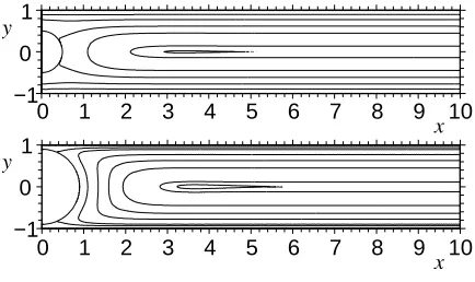
If the vertical scale is expanded twentyfold, as in Fig. 7(a), it is possible to resolve the first saddle point (labelled A), and the basic separatrix structure identified earlier. Given the predicted velocity damping ratio, however, it is hardly surprising that the next separatrix structure appears only as a horizontal line lying between the stream-lines forming the larger separatrix. Fig. 7(b) is a plot with a further exaggeration in the vertical direction, which reveals that the horizontal line of Fig. 7(a) is indeed another separatrix structure nested withing the first.

As an alternative means of demonstrating the existence of the stagnation-point chain, Fig. 8 shows plots of the vertical velocity component along the curve u = 0 for the same flow conditions as in Fig. 7 (and the lower plot in Fig. 6). The upper graph in Fig. 8 shows that the velocity decays very rapidly, but the inset plot reveals that this decay is not monotonic: the velocity vanishes (at x≈ 3.7, corresponding to the first centre), then becomes negative, and decreases to a minimum before again approaching zero. The lower plot in Fig. 8, focusing on the range −3×10−11 _{6 v 6 3×10}−11_, confirms that the velocity switches sign several times as it decays. An advantage of plotting the velocity component along u= 0 is that it is easy to compare the values obtained using the finer mesh mentioned above: the fine-mesh data are included in Fig. 8 as the small black circles, and show that even on the expanded scale there is no discernible difference in the calculated velocity.

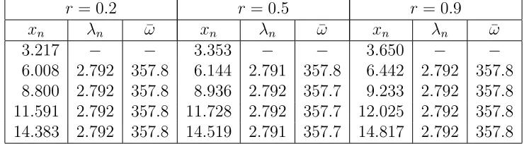
The other feature of note in Fig. 8 is that the separation between consecutive stag-nation points appears to be constant. Tables 1–4 explore this further, and present the x-coordinates of stagnation points together with calculations of the separation of consecutive points and the corresponding damping ratio for various values of the four key parameters in the problem: r,yc, ˙γc, andRe. As stated above, these results

domain).

As is to be expected, the presence of fluid inertia has a marked effect on the damping ratio, as shown in table 4. IncreasingRealso has the effect of increasing the separation of the stagnation points. However, both λn and ¯ω remain constant for a given chain

of stagnation points. Fig. 10 shows a plot of the variation of λn and ¯ω withRe. After

a very slight decrease at small Re, λn increases with Re, however ¯ω exhibits a much

more pronounced decrease to a minimum atRe≈38, before increasing monotonically with Re. The decrease in velocity ratio with smallReseems intuitive if one associates an increase inRewith a reduction in viscous damping. On the other hand, one would expect that greater fluid inertia would cause the influence of the cylinder to become more localized; hence ¯ω ultimately increases with Re.

IV

The half-filled annulus revisited

Consider an annulus between coaxial cylinders which is completely filled with fluid. If the cylinders are slowly rotated in opposite directions, the resulting streamlines would be circular, and somewhere between the cylinder surfaces would be a streamline along which the fluid velocity vanishes. Though circular, this will be referred to as a ‘stagnation line’, as it corresponds to those seen in the planar flows considered earlier.

Now, if the annulus were filled to a level between the topmost and lowest points on the inner cylinder, a free surface would be present on either side of the inner cylinder19_. When the cylinders are again rotated in opposite directions, the free surfaces become obstacles to the flow, causing some (or all29_{) of the fluid to turn around. In the} light of Sec. II, the expected flow structure in each half of the domain is a chain of stagnation points with separatrices nested as in Fig. 4(d) or (f), which allow the effect of the two-dimensional disturbance to diminish with distance from each free surface. Since the (Stokes) flow is symmetric, the i’th saddle point in the left-hand half of the domain (counting from the free surface) must be connected to the i’th saddle in the right-hand half. This results in the nested sequence of treble-eddy structures shown in Fig. 3(e).

A

The effect of eccentricity

However, the flow will be fundamentally changed if the gap between the cylinders is made non-uniform. This can easily be achieved by displacing the cylinders relative to each other, so that the annulus becomes eccentric. For convenience this displacement is taken to be along the centreline of the half-annulus, so that the geometry is still symmetrical, see Fig. 11. This allows the effects of eccentricity to be explored by perturbing the concentric-cylinder solution of Gaskellet al.19. The eccentric model is based on the same assumptions19_{: the liquid is Newtonian, with constant density and} viscosity; the cylinders are assumed to dewet as they rotate, so no liquid films are withdrawn from the bulk; the flow is sufficiently slow for inertia effects to be negligible; and the free surfaces are modelled as radial (with respect to the inner cylinder) stress-free planes inclined at an angle determined by a balance of hydrodynamic and hydrostatic pressures19_.

If the centre of the inner cylinder is taken as the origin of the polar coordinate system (R, θ), and the axis of the outer cylinder is displaced upwards a distance E along the centreline θ = 0, it can be shown that the equation for the surface of the outer cylinder is

¯

r0(θ) = −Ecosθ+ q

E2_(cos2_{θ−1) +R}2

0, (12)

where E is the displacement of the centres of the cylinders and R0 is the radius of the outer cylinder. Scaling lengths by the radius of the inner cylinder, Ri, (12) can

be written as

r0 ≡ ¯

r0

Ri

=−εcosθ+ ¯R

q

ε2_/R¯2_(cos2_{θ−1) + 1 = ¯R−εcosθ+O(ε}2_{), (13)}

where ¯R =Ro/Ri is the radius ratio. A solution to the biharmonic equation is sought

by expanding the (dimensionless) streamfunction,ψ, in powers of ε:

ψ =ψ0+εψ1+O(ε2), (14)

and so the boundary conditions must also be expanded to give

ψ = ∂ 2_ψ

∂θ2 = 0 on θ=±π/2, (15)

ψ = ∂ψ

∂θ = 0; ∂ψ

∂r = 1 on r= 1, (16)

ψ = 0; 1

r ∂ψ ∂θ =−

S

¯

Rεsinθ; ∂ψ

∂r =S(1 +O(ε

2_{)) on r =r}

0(θ), (17)

whereS =Uo/Ui is the outer to inner peripheral speed ratio of the cylinders (Ui being

the velocity scale for the problem), and r is the dimensionless radial coordinate. The boundary conditions on r = r0(θ) are imposed with reference to r = ¯R by means of Taylor series, for example

ψ|r=r0 =ψ|r= ¯R−εcosθ

∂ψ ∂r

r= ¯R

Substituting (14) into (18) and using the first condition in (17) then gives

0 = ψ0+εψ1−εcosθ

∂ψ0

∂r onr = ¯R. (19)

The other conditions in (17) are similarly treated, and comparing the coefficients of

ε then gives a sequence of boundary value problems. The O(1) problem for ψ0 is of course identical to the concentric case19_{, while the O(ε) problem has conditions}

ψ1 =

∂2_ψ 1

∂θ2 = 0 on θ =±π/2, (20)

ψ1 =

∂ψ1

∂r =

1

r ∂ψ1

∂θ = 0 on θ=±π/2, (21)

and, onr= ¯R,

ψ1 = cosθ

∂ψ0

∂r , (22)

∂ψ1

∂r = cosθ ∂2_ψ

0

∂θ2 , (23)

1

r ∂ψ1

∂θ = − S

¯

Rsinθ+

cosθ r

∂2_ψ 0

∂r∂θ. (24)

The nature of the O(ε) boundary conditions indicate that ψ1 should have the form

ψ1 ∼f(r, θ) cosθ, but a solution of the biharmonic equation satisfying the boundary conditions can only be found if f is independent of θ. This is, in fact, not an un-reasonable assumption since, close to the cylinder surfaces, variations of ψ0 and its derivatives are negligible except very near the interfaces. As the region of interest is the core of the domain, advantage can be taken of this fact to simplify the O(ε) boundary conditions. Assuming purely azimuthal flow, then, the velocity profile is

v(r) = arlnr+br+c/r, (25)

where

a = 2(1−RS¯ −R¯

2_+SR¯3_{−2SR¯ln ¯R+ 2 ¯R}2_{ln ¯R)} ( ¯R2_{+ 2 ¯Rln ¯R−1)( ¯R}2_{−2 ¯Rln ¯R−1)} ,

b = SR¯−1−aR¯ 2_{ln ¯R} ¯

R2₋₁ ,

c = aR¯

2_{ln ¯R+ ¯R}2_−SR¯ ¯

R2₋₁ . Using (25), conditions (22)–(24) simplify to

ψ1 =Scosθ,

∂ψ1

∂r =a(1 + lnr+b−c/r

2_{) cosθ,} ∂ψ1

∂θ =−Ssinθ (26)

on r= ¯R. The resulting O(ǫ) correction to the concentric streamfunction is then

where

A = R¯

4_{+ 2SR}¯3_{ln ¯R−2SR}¯3_{−4 ¯R}2_{ln ¯R+ 2 ¯RS −1 + 2SR}¯_{ln ¯R} ( ¯R2_{+ 2 ¯Rln ¯R−1)( ¯R}2_{−2 ¯Rln ¯R−1)( ¯R}2₋₁₎ ,

B = −R¯( ¯R

3 _{+ 2SR}¯2_{ln ¯R−SR}¯2_−R¯_{−2 ¯Rln ¯R+S)} ( ¯R2 _{+ 2 ¯Rln ¯R−1)( ¯R}2 _{−2 ¯Rln ¯R−1)( ¯R}2₋₁₎ ,

C = 1−RS¯ −R¯

2_+SR¯3_−2SR¯_{ln ¯R+ 2 ¯R}2_{ln ¯R} ( ¯R2_{+ 2 ¯Rln ¯R−1)( ¯R}2_{−2 ¯Rln ¯R−1)( ¯R}2₋₁₎,

D = −2( ¯R

2_{+ 2SR}¯_{ln ¯R−1)}

( ¯R2_{+ 2 ¯Rln ¯R−1)( ¯R}2_{−2 ¯Rln ¯R−1)}.

When ¯R = 1.5 and S = 0, the flow in the concentric annulus features the treble-eddy structure sketched in Fig. 3(b), and Fig. 12 shows how the position of each stagnation point changes as the eccentricity of the cylinders increases. At ε ≈ 9.02×10−7 _a pitchfork-type bifurcation transforms the centre onθ= 0 into a saddle and produces two new centres, which move apart asε increases. Meanwhile the two original saddle points move inwards, and at ε≈2.385×10−5 _{two saddle-node bifurcations occur, in} which each new centre coalesces with one of the saddle points, to leave a double-eddy structure.

A check of the streamfunction values at each stagnation point confirms that the sequence of structural changes is as indicated by the schematics in Fig. 12. At

ε ≈ 1.91× 10−5_{, the three saddle points link in a parametrically unstable} four-eddy structure, after which the flow structure becomes as in Fig. 3(f). These flow structures are all consistent with the general analysis of Brøns and Hartnack10_{, and} appear in their Fig. 7(a) (if one connects up the ‘unfinished’ separatrices). Evidently when the annulus is eccentric, the ‘pinching’ effect of the cylinder surfaces favours the structures having a double-eddy outer separatrix, as seen in Fig. 11, and the values of ε cited above indicate that only a very small eccentricity is required to destroy the structure seen in the uniform-gap flow.

V

Conclusion

It has been shown that when a bounded shear flow featuring a stagnation line is disturbed, for example by the presence of an obstacle in the flow, the stagnation line is replaced by a chain of stagnation points and a nested separatrix structure.

Each saddle point has associated with it a homoclinic streamline enclosing an eddy around the centre immediately before it (i.e. nearer to the disturbance), and two streamlines which extend to infinity and eventually become parallel. The decaying form of the streamfunction dictates that the closed eddy attached to each saddle point lies between the ‘open’ streamlines of the saddle immediately before, thus forming a ‘nested’ structure. When the Couette flow is anti-symmetric, i.e. when the plate velocities are equal but opposite, the stagnation points appear along the original stagnation line. However, when the stagnation line does not lie exactly halfway between the plates, the resulting stagnation points are displaced such that the elliptic and hyperbolic points appear on opposite sides of the stagnation line. The resulting flow structure is topologically the same, however.

Finite element calculations of shear flow past a stationary circle confirm the predic-tions of the superposition, and for Stokes flow produce stagnation point separapredic-tions and velocity damping ratios very close to those predicted analytically. The results show that these values are independent of the size and position of the cylinder, sup-porting the conclusion that the flow structure described above is a general response of a parallel shear flow to a two-dimensional disturbance. The sequence of stagnation points forms an ‘approximation’ of the stagnation line, while the nested separatrix structure allows the two-dimensional flow caused by the disturbance to diminish with distance so that the flow approaches parallel shear flow far from the disturbance.

Variation of the Reynolds number showed that the separation between stagnation points increases withRe (after a very slight decrease at smallRe), while the velocity damping ratio shows a pronounced decrease to a minimum at Re≈38 before increas-ing monotonically. However, for each value of Re, these quantities remain constant along the whole stagnation point chain.

The effect of a non-uniformity in the gap between the plates driving the shear flow was explored by perturbing the concentric half-filled annulus problem of Gaskell et al.19 to allow for a symmetrical eccentricity in the cylinder positions. It was shown that only a small eccentricity is required to destroy then chain of stagnation points present when the gap is uniform. However, for very small eccentricities, additional flow structures can be seen, which were predicted by the bifurcation theory of Brøns and Hartnack10 _{but were absent in the concentric annulus}19 _{due to the uniformity of} the gap between the cylinders.

References

1_{A. E. Perry and D. K. M. Tan, “Simple three-dimensional motions in coflowing jets}

and wakes,” J. Fluid Mech. 141, 197–231 (1984)

2_{S. C. Jana, G. Metcalfe and J. M. Ottino, “Experimental and computational studies}

of mixing in complex Stokes flows: the vortex mixing flow and multicellular cavity flows,” J. Fluid Mech. 269, 199–246 (1994)

3_{M. C. T. Wilson, P. H. Gaskell and M. D. Savage, “Flow in a double-film-fed fluid}

bead between contra-rotating rolls. Part 1: Equilibrium flow structure,” Euro. J. Appl. Math. 12, 395–411 (2001)

4_{J. L. Summers, H. M. Thompson and P. H. Gaskell, “Flow structure and transfer}

jets in a contra-rotating rigid-roll coating system,” Theor. Comput. Fluid Dyn. 17(3), 189–212 (2004)

5_{P. N. Shankar and M. D. Deshpande, “Fluid mechanics in the driven cavity,” Ann.}

Rev. Fluid Mech. 32, 93–136 (2000)

6_{F. G¨urcan, P. H. Gaskell, M. D. Savage and M. C. T. Wilson, “Eddy genesis and}

transformation of Stokes flow in a double-lid-driven cavity,” Proc. Instn Mech. Engrs Part C: J. Mech. Eng. Sci. 217, 353–364 (2003)

7_{M. Tobak and D. J. Peake, “Topology of three-dimensional separated flows,” Ann.}

Rev. Fluid Mech. 14, 61–85 (1982)

8_{A. E. Perry and M. S. Chong, “A description of eddying motions and flow patterns}

using critical-point concepts,” Ann. Rev. Fluid Mech.19, 125–155 (1987)

9_{P. G. Bakker, Bifurcations in flow patterns (Kl¨uwer Academic, 1991).}

10_{M. Brøns and J.N. Hartnack, “Streamline topologies near simple degenerate critical}

points in two-dimensional flows away from boundaries,” Phys. Fluids11(2), 314– 324 (1999)

11_{F. P. Bretherton, “Slow viscous motion round a cylinder in a simple shear,” J. Fluid}

Mech.12, 591–613 (1962)

12_{R. G. Cox, I. Y. Z. Zia and S. G. Mason, “Particle motions in sheared suspensions.}

XXV. Streamlines around cylinders and spheres,” J. Colloid Interf. Sci. 27(1), 7–18 (1968)

13_{C. R. Robertson and A. Acrivos, “Low Reynolds number shear flow past a rotating}

14_{C. A. Kossack and A. Acrivos, “Steady simple shear flow past a circular cylinder}

at moderate Reynolds numbers: a numerical solution,” J. Fluid Mech. 66(2), 353–376 (1974)

15_{D. J. Jeffrey and J. D. Sherwood, “Streamline patterns and eddies in}

low-Reynolds-number flow,” J. Fluid Mech. 96(2), 315–334 (1980)

16_{E. J. Ding and C. K. Aidun, “The dynamics and scaling law for particles suspended}

in shear flow with inertia,” J. Fluid Mech. 423, 317–344 (2000)

17_{C. M. Zettner and M. Yoda, “The circular cylinder in simple shear at moderate}

Reynolds numbers: an experimental study,” Exp. Fluids30, 346–353 (2001)

18_{B. Martin, “Numerical studies of steady-state extrusion processes”, PhD thesis,}

Cambridge University (1969)

19_{P. H. Gaskell, M. D. Savage and M. Wilson, “Stokes flow in a half-filled annulus}

between rotating coaxial cylinders,” J. Fluid Mech.337, 263–282 (1997)

20_{R. Kidambi and P. K. Newton, “Steamline topologies for integrable vortex motion}

on a sphere,”Physica D,140, 95–125 (2000)

21_{H. K. Moffatt, “Viscous and resistive eddies near a sharp corner,” J. Fluid Mech.}

18, 1–18 (1964)

22_{M. Hellou and M. Coutanceau, “Cellular Stokes flow induced by rotation of a}

cylin-der in a closed channel,” J. Fluid Mech.236, 557–577 (1992)

23_{M. Hellou, “Sensitivity of cellular Stokes flow to geometry,” Eur. J. Phys.22, 67–77}

(2001)

24_{W. W. Hackborn, “Asymmetric Stokes flow between parallel planes due to a rotlet,”}

J. Fluid Mech. 218, 531–546 (1990)

25_{P. Carbonaro and E. B. Hansen, “Transient Stokes flow in a channel driven by}

moving sleeves,” J. App. Mech.57, 1061–1065 (1990)

26_{S. F. Kistler and P. M. Schweizer (eds.), Liquid Film Coating (Chapman & Hall,} London, 1997)

27_{T. C. Papanastasiou, N. Malamataris and K. Ellwood, “A new outflow boundary}

condition,” Int. J. Numer. Meth. Fluids 14, 587–608 (1992)

28_{S. F. Kistler and L. E. Scriven, “Coating flows,” in “Computational analysis of}

polymer processing” (eds. J. R. A. Pearson and S. M. Richardson), pp. 243–299, London: Applied Science (1983)

r= 0.2 r = 0.5 r= 0.9

xn λn ω¯ xn λn ω¯ xn λn ω¯

3.217 − − 3.353 − − 3.650 − −

6.008 2.792 357.8 6.144 2.791 357.8 6.442 2.792 357.8 8.800 2.792 357.8 8.936 2.792 357.7 9.233 2.792 357.8 11.591 2.792 357.8 11.728 2.792 357.7 12.025 2.792 357.8 14.383 2.792 357.8 14.519 2.791 357.7 14.817 2.792 357.8

yc = 0.1 yc = 0.2 yc = 0.3

xn λn ω¯ xn λn ω¯ xn λn ω¯

3.330 − − 3.288 − − 3.249 − −

6.122 2.792 357.8 6.080 2.792 357.7 6.040 2.792 357.7 8.913 2.792 357.8 8.872 2.792 357.7 8.832 2.792 357.7 11.705 2.792 357.8 11.663 2.792 357.7 11.624 2.792 357.7 14.497 2.792 357.8 14.455 2.792 357.7 14.415 2.792 357.7

˙

γc = 1.5 γ˙c = 2.0 γ˙c = 2.5

xn λn ω¯ xn λn ω¯ xn λn ω¯

3.314 − − 3.265 − − 3.225 − −

6.113 2.799 361.8 6.074 2.809 367.1 6.042 2.817 371.5 8.905 2.792 357.7 8.866 2.792 357.7 8.834 2.792 357.7 11.697 2.792 357.7 11.658 2.792 357.7 11.626 2.792 357.7 14.488 2.791 357.7 14.448 2.791 357.7 14.418 2.792 357.7

Re= 10 Re= 20 Re= 30

xn λn ω¯ xn λn ω¯ xn λn ω¯

3.352 − − 3.508 − − 3.766 − −

6.171 2.819 172.7 6.675 3.166 100.6 7.457 3.690 84.6 8.989 2.818 172.7 9.841 3.166 100.8 11.148 3.692 85.1 11.806 2.818 172.7 13.010 3.166 100.8 14.840 3.692 85.1 14.624 2.818 172.7 16.172 3.166 100.8 18.532 3.692 85.1

Figure captions

Fig. 1. Three of the five flow structures presented by Jeffrey and Sherwood15 _{in an} unbounded shear flow past a cylinder: (a) stationary cylinder, (b) cylinder rotating more slowly than a freely rotating one, (c) cylinder freely rotating.

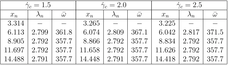
Fig. 2. The four possibilities for blocked flow identified by Jeffrey and Sherwood15_.

Fig. 3. A selection of flow structures illustrating different ways in which a chain of a given number of stagnation points can be connected together. Patterns (a)–(e) were observed by Gaskell et al.19 _{in their annular geometry; (f)–(h) are theoretically} possible in viscous flow according to the analysis of Brøns and Hartnack10_{. Similar —} and indeed more complex streamline patterns — also arise in inviscid vortex flows20_.

Fig. 4. Response of flow between infinite parallel plates to an arbitrary distant dis-turbance: (a) the sequence of eddies identified by Moffatt20_{, including as an example} of a disturbance a rotating cylinder; (b) the superposition of Moffatt’s solution with a symmetric Couette flow; (c) a sketch (not to scale) of the decay of the stream-function along the line y = 0; (d) the deduced flow structure; (e) superposition of Moffatt’s solution with an asymmetric Couette flow; (f) the deduced asymmetric flow. Throughout the diagrams elliptic (centre) stagnation points are shown as •, hyper-bolic (saddle) points as ×, and eddy centres as +. The horizontal dashed line in the flow schematics indicates the position of the stagnation line in the Couette flow.

Fig. 5. Illustration of the computational mesh construction.

Fig. 6. Streamline plots showing a closed eddy surrounding the first elliptic stagnation point in the chain predicted by the Couette-Moffatt superposition. In the top plot

r= 0.5, while in the bottom r = 0.9; in both ˙γ = 1.0,yc = 0, and Re= 0.

Fig. 7. Streamline plots showing the nested separatrix structure. The vertical scale has been exaggerated in both plots. Plot (a) shows the first centre and saddle point, which form the basic nested structure; (b) is a further expanded view showing the second centre-saddle pair and how it lies nested within the first structure. Parameter values: r= 0.9, ˙γ = 1.0, yc = 0, and Re= 0.

Fig. 8. Variation of the vertical velocity component, v, versus horizontal distance along the curve u = 0 on the right-hand side of the cylinder. Parameter values:

r = 0.9, ˙γ = 1.0, yc = 0, and Re= 0.

Fig. 9. Expected structure of blocked flow when confining plates are present.

Fig. 10. Effect of Re on the separation, λn, and the velocity damping ratio, ¯ω, of

adjacent stagnation points. In this case r= 0.5, ˙γ = 1.0, and yc = 0.

(b)

(c) (a)

(d) (c)

(a) (b)

(g) (f) (a)

(c)

(d) (b)

(e) (h)

00000000000000000

11111111111111111

00000000000000000

11111111111111111

00000000000000000

00000000000000000

11111111111111111

11111111111111111

00000000000000000

11111111111111111

00000000000000000

00000000000000000

11111111111111111

11111111111111111

00000000000000000

11111111111111111

00000000000000000

00000000000000000

11111111111111111

11111111111111111

00000000000000000

00000000000000000

11111111111111111

11111111111111111

00000000000000000

11111111111111111

00000000000000000

00000000000000000

11111111111111111

11111111111111111

(c) (b) (a)

(d)

(e)

(f)

x

ψ y

u=−1

boundary condition condition

u=S

free

y_i u=0

no slip

x=0 r

no slip

yc y=0

u=0 free boundary

y

y

x x 0

0 1

1 1

0

10 9 8 7 6 5 4 3 2 1

−1

2 3 4 5 6 7 8 9 10

0

−1

3 4 5 6

6

7 8 9 10 11 12 13 14

15 15

7 8 9 10 11 12 13 14

x −1.00

−0.75 −0.50 −0.25 0.00 0.25 0.50 0.75 1.00

20y

−0.75 −0.50 −0.25 0.00 0.25 0.50 0.75

500y

A

(b) A

(a)

0 0.1 0.2 0.3 0.4

v

0 2 4 6 8 10 12 14 16 18 20

x -2×10-11

0 2×10-11

v

4 6 8

x -0.001

0 0.001

v

0 10 20 30 40 50 60

Re

2 3 4 5 6

λ_n

100 150 200 250 300 350 400

ω

R E

r Ri

o

o θ

0 1x10−5 2x10−5 3x10−5

ε

−π/2 −π/4 0

π/4

π/2

θ