Kinematics Based Analytical Solution for Wheel Slip Angle Estimation of a RWD Vehicle with Drift

Article

Kinematics-Based Analytical Solution for Wheel Slip

Angle Estimation of a RWD Vehicle with Drift

Ronnapee Chaichaowarat

_{and Witaya Wannasuphoprasit}

_*

Department of Mechanical Engineering, Faculty of Engineering, Chulalongkorn University, 254 Phayathai Road, Pathumwan, Bangkok 10330, Thailand

E-mail: a_{[email protected],} b_{[email protected] (Corresponding author)}

Abstract. Accurate real-time information of wheel slip angle is essential for various active stability control systems. A number of techniques have been proposed to enhance quality of GPS based estimation. This paper exhibits a novel cost-effective strategy of individual wheel slip angle estimation for a rear-wheel-drive (RWD) vehicle. At any slip condition, the slip angle can be estimated using only measurement of steering angle, front wheel rolling speeds, yaw rate, longitudinal and lateral accelerations, without requiring GPS data. On the basis of zero longitudinal slip at the both front tires, the closed-form solutions for direct computation of wheel slip angles were derived via kinematic analysis of a planar four-wheel vehicle, and then primarily verified by computational simulation with prescribed functions of radius of curvature, vehicle speed, sideslip and steering angle. Neither integration nor tire friction model is required for this estimation methodology. In terms of implementation, a 1:10th scaled RWD vehicle was modified so that the steering angle, the front wheel rolling speeds, the vehicle yaw rate and the linear accelerations could be measured. Preliminary experiment was done on extremely random sideslip maneuvers beneath the global positioning using four recording cameras. By comparing with the vision-based reference, the individual wheel slip angles could be well estimated despite extreme tire slip. Other vehicle state variables—i.e., radius of curvature, vehicle sideslip and speed—might be obtained from kinematic relations. This proposed estimation methodology could then be alternatively applied for the full range slip angle estimation in advanced chassis control applications.

Keywords: Vehicle dynamics, state estimation, chassis control systems, slip angle, sideslip.

ENGINEERING JOURNAL Volume 20 Issue 2 Received 22 May 2015

Accepted 4 November 2015 Published 18 May 2016

1.

Introduction

Nowadays, a number of active safety systems for vehicle motion control have been successively developed by several automobile manufacturers and commercialized into general modern passenger cars in order to improve driving performance, stability and controllability despite emergency extreme slip maneuvers. All of the existent advanced chassis control applications such as the vehicle stability control system or electronic stability program (ESP) [1, 2], the vehicle dynamics control system (VDC) [3], the yaw stability control system (YSC) and some other systems [4, 5] determine their control algorithms by feedback of some dynamic state variables e.g., lateral acceleration, vehicle yaw rate and sideslip. Since performances of such the systems could be dramatically improved from more accurate state information, great endeavor is being directed towards developing reliable state estimation methodologies.

Using micro-electro-mechanical systems (MEMs) accelerometer and gyroscope, the lateral acceleration and the vehicle yaw rate could be directly measured respectively. However the obtained yaw rate usually contains significant error. In practical, the yaw rate was generally estimated via application of a global positioning system (GPS) with fusing of some on-vehicle sensors—e.g., steering angle sensor, ABS wheel-speed sensors, and inertial measurement unit (IMU), as proposed in the automotive navigation systems [6– 8]. These sensors offer little correction to the GPS position solution; however, are primarily required when GPS data is unavailable such as between tall buildings, underneath trees, inside a parking structure and under a bridge. On the basis of zero sideslip, the estimator developed in [6] used GPS heading and velocity to estimate rear wheel radii while the GPS signal was available by taking ratio of the GPS velocity and wheel angular velocities followed by using the obtained wheel radii to estimate the heading while GPS signal was unavailable.

Vehicle sideslip is the angle the vehicle velocity makes with its longitudinal axis at the center of gravity whereas the wheel slip angle is the angle between the tire velocity vector and the wheel direction [9]. Since too high slip angle could reduce the tire ability to generate lateral tire force, slip angle control system for preventing sideslip from becoming too large is undoubtedly crucial. Not only the vehicle yaw rate but also the sideslip are required for control logics of the systems [10–12], especially for the slip angle control system [2]. Although the vehicle sideslip might be obtained from application of an optical or a radar Doppler speed-over-ground sensor [13, 14], both equipment are still considered as so expensive for ordinary automotive applications as mentioned in [15, 16].

In order to compensate the lack of direct measurement due to current technical constraints, sideslip estimation strategies by integrating two-antenna GPS with some typical on-vehicle sensors available for chassis control applications are the current state-of-the-art. A number of techniques have been proposed to enhance quality of the GPS-based sideslip estimation. For example, the vehicle sideslip was estimated from the different angle between a GPS velocity heading and a yaw heading integrated from gyro measurement in [17] via a kinematic Kalman filter. Building on the framework of [17], another model-based Kalman filter with correctly identified vehicle model parameters was developed in [18] to estimate not only sideslip but also yaw rate and tire cornering stiffness from the measured steering angle and GPS heading, despite time-varying weight distribution and tire friction coefficient. In addition, sideslip estimation was used to estimate vehicle roll parameters in [19] and was applied for the vehicle stability control system in [20]. Later, the combination of the GPS-based and the model-based observer for sideslip estimation was proposed in [15] where the GPS was firstly employed to estimate gyro bias during straight driving. Primarily, sideslip was estimated by comparing the GPS course angle to the gyro heading integrated from the yaw rate. Accurate sideslip was obtained from the designed linear observer the states of which were vehicle heading and gyro bias whereas the input was the measured yaw rate. Lastly, the high update rate estimation of vehicle sideslip, tire slip angle and vehicle attitude, which could overcome the effect of vehicle roll and road slant, was developed in [16] where the vehicle roll and heading were measured by a two-antenna GPS. The vehicle sideslip estimated via a kinematic Kalman filter was used to identify the tire cornering stiffness; also, the bicycle model parameters were estimated from a separated algorithm.

surfaces. However, integration of noise signals or bias sensing error might cause accumulated error as drift; also, vehicle roll and road bank angle could affect the accuracy of estimation. On the other hand, the model-based method which estimates sideslip via various types of observer [24, 25] is relatively robust against sensing error and noise signals; moreover, it can overcome the error due to vehicle roll and road bank. However, the quality of estimation strongly depends on the accuracy of the vehicle and tire model parameters. Since most of the model-based estimation methods—i.e., linear state observer [26, 28] and Kalman filter—relying on a linear vehicle model can work efficiently only under nominal vehicle operating conditions where tires operate within the linear slip-friction characteristic but no longer work reliably when the vehicle is skidding and the slip angle becomes large, other types of observer developed based on the extended nonlinear vehicle model such as nonlinear observer [29–33], extended Kalman filter [34], extended Luenberger observer and sliding-mode or adaptive observer have been proposed to overcome these constraints caused by the nonlinear tire characteristic. Nevertheless, these methods are too complicated and still have large error due to model parameters mismatching. In spite of estimation difficulties due to influence of relative road slant and nonlinear tire characteristic, the combination of both kinematics-based method and model-based method has been proposed as the combined method [3, 5, 35– 41]. Furthermore, an alternative direct virtual sensor (DVS) [42, 43] was designed, based on the idea of a two-step procedure: direct identifying vehicle model exploiting measurement of on-vehicle sensors and observer design based on the estimated model, for sideslip estimation of general vehicle.

In this manuscript, a novel concept of kinematics-based analytical closed-form solution which could provide the cost-effective estimation methodology for the individual wheel slip angle of a rear-wheel-drive (RWD) vehicle will be proposed. At any slip condition, the slip angle can be estimated using only the measured data of steering angle, front wheel speeds, vehicle yaw rate, longitudinal and lateral accelerations, without requiring GPS data. Since neither vehicle nor tire friction model is used in the estimation, both the error due to inaccuracy of model parameter and the error caused by extreme slip maneuver could be completely avoided. Besides, accumulation of gyro bias sensing error will not appear because no integration is required. However, appropriate filter is still needed for practical usage because the errors caused by measurement inaccuracies of the yaw rate and the accelerations are always present. From the obtained wheel slip angles, all dynamic state variables—i.e., radius of curvature, vehicle sideslip and speed—could be directly computed through kinematic relations. The proposed estimation concept could then be alternatively applied for the full range slip angle estimation in various chassis control applications dealing with extreme tire slip. For example, the automatic drifting controller [44] developed on the basis of steady state drifting dynamics proposed in [45] and [46] accordingly.

In the entire of this paper, derivation of the kinematics-based analytical closed-form solution for an individual free-rolling front wheel slip angle, written as a function of some measurable dynamic variables— i.e., steering angle, front wheel rolling speeds, vehicle yaw rate, longitudinal and lateral accelerations, will be firstly described followed by the kinematic relations used for ensuing estimation of the both rear wheel slip angles. The results of computational validation for the obtained analytical solutions will be shown. After that, specification of the developed 1:10th _{scaled testing vehicle used for preliminary implementation and} experiment will be briefly depicted, followed by the verification results of the developed estimation strategy.

2.

Kinematics-Based Analytical Closed-Form Solution

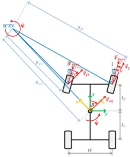
from the ICZV to the ground contact points of the front left and front right wheels are denoted by and respectively. The vehicle velocity ⃗ is perpendicular to the direction of the relative distance . The angle from the instant vehicle heading to the direction of the vehicle velocity ⃗ is denoted by the vehicle sideslip measured positive in the clockwise direction. Likewise, the local velocities of the front left wheel

⃗ and of the front right wheel ⃗ are perpendicular to the directions of the relative distances and respectively. The front left wheel slip angle and the front right wheel slip angle are the angles measured in the clockwise direction from the instant wheel rolling directions to the front left wheel velocity

⃗ andto the front right wheel velocity ⃗ respectively. The steering angle measured from the vehicle heading direction to the wheel rolling direction is also positive in the clockwise direction. Finally, the local velocities of the front left wheel ⃗ and of the front right wheel ⃗ can be decomposed into the components in the wheel rolling directions as ⃗ and ⃗ respectively.

Fig. 1. Schematic diagram of a four-wheel vehicle cornering on plane.

2.1. Estimation of Front Wheel Slip Angles

Derivation of the kinematics-based analytical closed-form solutions for the individual free-rolling front wheel slip angles, written as functions of the steering angle control input and some measurable dynamic variables—i.e., the front wheel rolling speeds and , the vehicle yaw rate ̇, the longitudinal acceleration and the lateral acceleration —will be described in this section.

Firstly, let us consider the vehicle velocity at the CG, magnitudes of the longitudinal and lateral velocities can be written as expressions of the vehicle speed sideslip as Eq. (1) and Eq. (2).

| ⃗ | (1)

Then, we consider the local velocities at the both front wheels, magnitudes of the front right and front left wheel velocities can be written as functions of the measurable wheel rolling speeds and the unknown wheel slip angles as Eq. (3) and Eq. (4) respectively.

| ⃗ | ⁄ (3)

| ⃗ | ⁄ (4)

The local velocities at the front right and front left wheels can be composed from the combination of the longitudinal and lateral components, corresponding to the magnitudes of the wheel steering angle and their unknown tire slip angles, as Eq. (5) and Eq. (6) respectively.

⃗ | ⃗ | ( ) ̂ | ⃗ | ( ) ̂ (5)

⃗ | ⃗ | ( ) ̂ | ⃗ | ( ) ̂ (6)

Since the wheel rolling speeds are simply obtained on the basis of zero longitudinal slip at the both front tires, we should remind that the obtained analytical solutions for direct computation of the individual wheel slip angles would attain accurate estimation only when no driving or braking torque is applied to the both front wheels.

In the following, the closed-form solution for estimation of the front right wheel slip angle will be derived. The vehicle velocity at CG can be composed from the front right wheel velocity and the relative velocity as Eq. (7). By substitution of Eq. (3) and Eq. (5) into Eq. (7), the vehicle velocity at CG can be written as Eq. (8). Thus, magnitudes of the longitudinal and lateral velocities are as Eq. (9) and Eq. (10) respectively.

⃗ ⃗ ( ̇ ̂) ( ̂ ̂) (7)

⃗ [

( ) ̇] ̂ [

( ) ̇] ̂ (8)

( ) ̇ (9)

( ) ̇ (10)

The squared magnitude of the vehicle velocity in Eq. (11) can be writtenas Eq. (12) by substitution of the longitudinal velocity magnitude from Eq. (9) and the lateral velocity magnitude from Eq. (10).

| ⃗ | (11)

| ⃗ | ̇( )

̇( ) ( ) ̇ (12)

Consider correlation between the moving frame coordinate and the moving frame coordinate; normal acceleration of vehicle can be written as a function of longitudinal acceleration, lateral acceleration and vehicle sideslip in Eq. (13). By neglecting the rate of change of the vehicle sideslip ( ̇ ), the normal acceleration can also be simply written as a function of the radius of curvature and the vehicle yaw rate in Eq. (14). By substitution of Eq. (14) into the left hand side of Eq. (13) and substitution of the trigonometric functions in the right hand side of Eq. (13) by the product of substitution Eq. (9) into Eq. (1) and the product of substitution Eq. (10) into Eq. (2), the correlation of normal acceleration can be written as Eq. (15)which can be transformed to Eq. (16).

(13)

̇ (14)

̇ [ ( ) ̇ | ⃗⃗ | ] [ ( ) ̇

| ⃗⃗ | ] (15)

| ⃗ | ̇ ( ) ( )

( ) ̇ (16)

By multiplying the yaw rate ̇ throughout Eq. (12), the obtained product can be equalized with Eq.(16). Then, the constructed equation can be simplified to the quadratic form in Eq. (17) with the coefficients prescribed by Eq. (18) to Eq. (20).

̇ (18)

[ ̇ ( ) ( )] (19)

[ ̇ ( ) ( )]

( ) ̇ ( ) ̇ (20) The roots of Eq. (17) can be simply obtainedfrom the quadratic formula in Eq. (21). The closed-from analytical solution for slip angle estimation of the front right wheel can be written as Eq. (22) with the coefficients prescribed in Eq. (18) to Eq. (20) consequently.

√

(21)

(

√

) (22)

Using similar way of derivation, the closed-form analytical solution for estimation of the front left wheel slip angle can also be obtained as written in Eq. (23) with the coefficients prescribed by Eq. (24) to Eq. (26).

(

√

) (23)

̇ (24)

[ ̇ ( ) ( )] (25)

[ ̇ ( ) ( )]

( ) ̇ ( ) ̇ (26)

From the measurable front wheel rolling speeds, steering angle and the obtained information of the both front wheel slip angles, magnitudes of the front right and left wheel velocities can directly be investigated by using Eq. (3) and Eq. (4) respectively. In addition, the velocity vectors at the both front wheels can be composed using Eq. (5) and Eq. (6). The other wheel slip angles at the both rear tires can also be derived via relative velocities as will be described.

2.2. Estimation of Rear Wheel Slip Angles

Derivation of the kinematics-based analytical closed-form solutions for the individual rear wheel slip angles, from the obtained information of the front wheel slip angles, will be described in this section.

The local velocity at the rear right wheel can be related to the front right wheel velocity through their relative velocity as the kinematic relation shown in Eq. (27). By substitution of Eq. (3) and Eq. (5) into Eq. (27), Eq. (28) can be attained and could then be transformed to Eq. (29). As a result, the rear right wheel slip angle can directly be estimated using information of the estimated front right wheel slip angle, the measurable front right wheel rolling speed and the steering angle consequently.

⃗ ⃗ ( ̇) ̂ ( ) ̂ (27)

⃗ [

( )] ̂ [

( ) ( ) ̇] ̂ (28)

(

( ) ( ) ̇

( )

) (29)

Using similar way of derivation, the closed-form analytical solution for estimation of the rear left wheel slip angle can also be obtained as Eq. (30) where the individual wheel slip angle can directly be estimated using information of the estimated front left wheel slip angle, the measurable front left wheel rolling speed and the steering angle eventually.

(

( ) ( ) ̇

( )

To summarize, the kinematics-based analytical closed-form solutions for slip angle estimation of the individual wheels—i.e., the front right wheel, the front left wheel, the rear right wheel and the rear left wheel—are proposed in Eq. (22), Eq. (23), Eq. (29) and Eq. (30) respectively.

3.

Computational Validation

In this section, primary validation of the previously derived closed-form solutions for the individual wheel slip angle estimation will be discussed. The verification was archived by computational simulation using MATLAB.

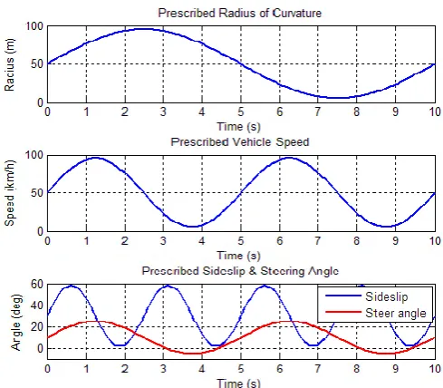
In the simulation, the steering angle control input and the three dynamic state variables—i.e., radius of curvature, vehicle speed and sideslip—were prescribed by sinusoidal functions with different amplitude and frequency as illustrated in Fig. 2. Between 10 seconds of the total simulation time period, the radius of curvature was varied from 5 meters to 95 meters. The vehicle speed was varied from 5 kilometers per hour to 95 kilometers per hour. The sideslip was varied from 2 degrees to 58 degrees in the clockwise direction whereas the steering angle was varied from 5 degrees in the counterclockwise direction to 25 degrees in the clockwise direction. The prescribed functions were specified to oscillate with different frequencies so that the simulated vehicle would incur with extremely random motion, as trajectory plotted on the horizontal

plane shown in Fig. 3. At the beginning of simulation, the vehicle was placed at the origin of the

global coordinate . The time interval taken for vehicle translation between any couple of adjacent points displayed in the figure was 0.5 seconds consistently.

As previously mentioned in the above that information of the steering angle and some measurable dynamic variables—i.e., the front wheel rolling speeds, the vehicle yaw rate, the longitudinal and the lateral accelerations—are required for the individual wheel slip angle estimation using the proposed kinematics-based analytical closed-form solutions. In this simulation, practical measurement of these dynamic variables was replaced by the direct computation from the prescribed functions using kinematic relations, as the results plotted in Fig. 4.

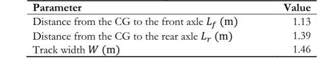
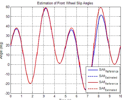
According to the prescribed function of steering angle and the obtained time-varying functions of the measurable dynamic variables, the individual wheel slip angles of the both front wheels can directly be estimated from the proposed Eq. (22) and Eq. (23). By using the vehicle parameters in Table 1, the front right wheel slip angle and the front left wheel slip angle were estimated and compared with the absolute velocity-based references computed from the magnitudes of the wheel longitudinal and lateral velocities, as the results exhibited in Fig. 5.

Table 1. The vehicle parameters used in this computational simulation.

Parameter Value

Distance from the CG to the front axle 1.13 Distance from the CG to the rear axle 1.39

Fig. 2. Prescribed functions of the steering angle control input and the three dynamic state variables.

Fig. 4. Necessary dynamic variables directly computed from the prescribed functions via kinematic relations.

Fig. 5. Estimated individual front wheel slip angles comparing with the absolute velocity-based references.

Consider the simulated estimation results in Fig. 5; both of the estimated front right wheel slip angle and the estimated front left wheel slip angle are completely fit with the absolute velocity-based references computed from the magnitudes of the wheel longitudinal and lateral velocities. However, there is another important notice of using these analytical closed-form solutions for the individual wheel slip angle estimation. According to the proposed Eq. (22) and Eq. (23), appropriate switching algorithm should be designated whether the square root value must be added to or subtracted from the first term. To summarize, the positive sign must be used in Eq. (22) if the value of in Eq. (19) is zero or positive. On the other hand, the negative sign must be used in Eq. (22) if the is negative. In a similar way, the positive sign must be used in Eq. (23) if the value of in Eq. (25) is zero or positive. On the other hand, the negative sign must be used in Eq. (23) if the is negative.

yaw rate, the longitudinal and the lateral accelerations—could not be obtained in common practice despite highly reliable measurement methods.

4.

Preliminary Implementation

In order to promote the proposed wheel slip angle estimation strategy for practical use, preliminary implementation must be examined. In this study, the testing system was developed on a 1:10th _scaled vehicle, the technical specification of which will be described in this section. Preliminary experiment was also done on extremely random sideslip maneuver beneath the global positioning. Details of the experimental setup will be briefly explained and followed by discussion of the testing results.

4.1. Testing Vehicle

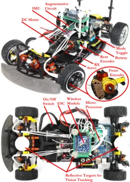
As previously specified that the kinematics-based closed-form solution for the wheel slip angle estimation was analyzed on the basis of zero longitudinal slip at the both front tires, the testing vehicle must be a rear-wheel-drive (RWD) platform with free-rolling front wheels. Since the testing vehicle was modified from the commercial 1:10th _{scaled radio controlled drifting chassis—namely HPI Pro-D Spec R—which is originally} four-wheel drive platform, the front-wheel driving mechanism must be firstly removed. In addition, appropriate on-vehicle sensors must be installed so that the real-time information of the steering angle control input and all necessary dynamic variables—i.e., the front wheel rolling speeds, the vehicle yaw rate, the longitudinal and the lateral accelerations—could be obtained. The perspective view of the testing vehicle, including an enlargement of the specially modified installation of front wheel speed encoders, is shown in the upper part of Fig. 6 and the top view is also shown in the lower part of the same figure.

Fig. 6. The modified 1:10th scaled RWD testing vehicle.

Reflective Targets for Vision Tracking ESC

DC Motor

Rear Encoder

Mode Toggle

On/Off Switch

Augmentative Circuit

Front Encoder RX

Servo

Battery

Micro Processor Wireless

To allow manual driving control following command signal of the Futaba 4PK-2.4G Super radio control transmitter (TX), standard components—i.e., the Futaba R614FF receiver (RX), the Vortex Experience electronic speed control (ESC) with brushless DC motor, the Futaba S3003 steering servo and the 7.4-volt Li-polymer battery—were primarily installed on the testing vehicle. To measure the front wheel rolling speeds, the US Digital EM 1-1-1250 encoders were modified and mounted into the both front wheels. Since a rear differential gear was always locked, the equivalent rear wheel rolling speeds could be measured by attaching the US Digital E4P 0.64”-300 encoder on the rear propeller shaft, in order to record data for further study. At the vehicle CG position projected on the horizontal plane, the ArduIMU+ V3 inertial measurement unit (IMU) was installed to provide the direct measurement of the vehicle yaw rate, the longitudinal and the lateral accelerations. The Arduino Mega 2560 ADK microcontroller board was used as the main processor of the testing vehicle. The XBee Pro 60mW Wire Antenna wireless module was applied to provide wireless communication with the outside stationary computer. Furthermore, the augmentative circuit was developed to support operation of the installed on-vehicle sensors. Two toggle switches were prepared for the adaptable controlling mode of the steering angle and the rear wheel speed, between manual control and automatic control. In order to support the vision-based object tracking application, the four reflective targets were carefully located on the testing vehicle so that their centroid position was coincident with the projection of the vehicle CG on the horizontal plane. The important parameters of the developed testing vehicle are shown in Table 2.

Table 2. Parameters of the modified 1:10th scaled RWD testing vehicle.

Parameter Value

Distance from the CG to the front axle 13.25 Distance from the CG to the rear axle 12.25

Track width 16.20

Wheel radius 3.25

4.2. Experimental Setup

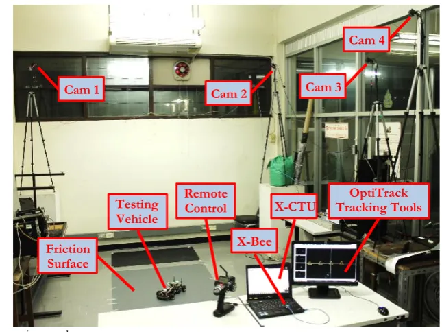
The preliminary experiment was done by controlling the testing vehicle manually through the radio control transmitter so that the vehicle performed random motion with extremely various sideslip around the prepared friction surface. During the test, the absolute position and the orientation of the testing vehicle were globally specified by using the Tracking Tools software working with the four OptiTrack-Flex3 commercial recording cameras, as the experimental setup shown in Fig. 7.

Fig. 7. The experimental setup.

Friction Surface

Testing Vehicle Cam 1

Cam 4

X-Bee

X-CTU Remote

Control

OptiTrack Tracking Tools Cam 3

In addition, the reference experimental time, the current sampling period and data measured by the installed on-vehicle sensors—i.e., the steering servo signal, the both front wheel rolling speeds, the rear propeller shaft speed, the IMU measured yaw rate, longitudinal and lateral accelerations—were automatically transferred to the data logger prepared on another computer through the X-Bee wireless communication modules working with the X-CTU software.

4.3. Experimental Results

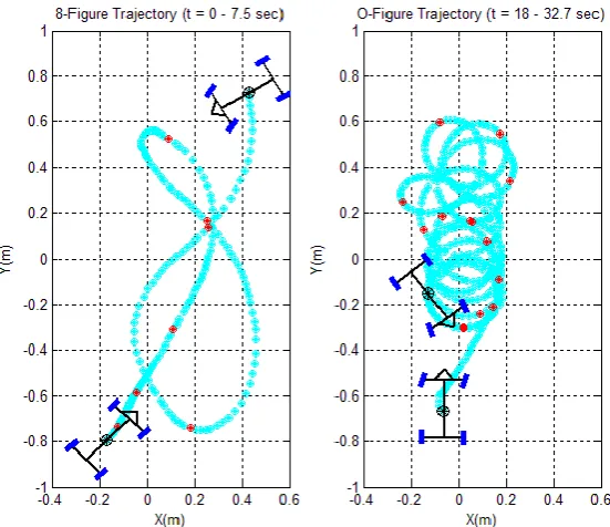
By using the data collected from the vision-based global positioning throughout the 40 seconds total experimental time period, the random motion trajectory of the testing vehicle, along with its corresponding orientation, can be plotted on the horizontal plane as shown in Fig. 8. In both plots of the figure, the sky dots represent the path of the vehicle CG position varying with time and the red dots emphasize the changing of the CG position in every second. In the first 20 seconds of the test, the vehicle was controlled to perform the 8-figure liked trajectory as illustrated in the left plot. The below vehicle mark indicates the starting point. The other vehicle mark shows a very large sideslip motion at the 7.5th _second. In the last 20 seconds of the test, the vehicle was controlled to perform the doughnut maneuver with the O-figure liked trajectory as illustrated in the right plot. The below vehicle mark indicates the transition state from the previous 8-figure maneuver to the doughnut maneuver at the 18th _{second. The other vehicle mark} at the 32.7th _{second shows that the testing vehicle was countersteering. At that time, the vehicle was} rotating in the CCW direction with the positive steering angle in the CW direction.

Fig. 8. The random motion trajectory of the testing vehicle.

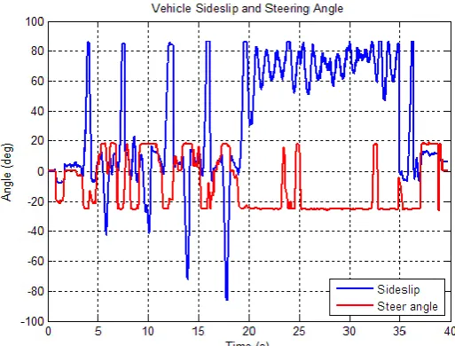
Using kinematic relations, the vehicle sideslip can directly be computed from the time-varying information of vehicle position and orientation, obtained from the vision-based global positioning. The global position-based vehicle sideslip and the time-varying steering angle obtained from the measured servo signal are plotted together in Fig. 9. According to the results, the steering angle was manually controlled to vary between 19 degrees in the CW direction and 22 degrees in the CCW direction so that the vehicle sideslip changed in the both CW and CCW directions. The angle of sideslip was sometimes so large that the magnitude could reach about 88 degrees. According to the plot of sideslip, this driving pattern could be inferred to be an extremely various sideslip maneuver.

cornering, as can be seen in the resulting plot between the 3rd _{second and the 37}th _{second. During the} 8-figure liked maneuver between the 3rd _{second and the 18}th _{second, the steering angle was switched between} the CW and the CCW directions in order to generate the corresponding yaw rate in the same directions whereas the sideslip was always changed to the opposite directions. During the CCW doughnut maneuver between the 18th _{second and the 37}th _{second, the steering angle was mostly controlled to be negative in the} CCW direction in order to generate the positive yaw rate in the CCW direction. With high speed cornering, the sideslip was always positive in the CW direction opposing from the steering angle and the yaw rate. The steering angle was sometimes controlled to be positive in the CW direction to perform countersteering while the testing vehicle was drifting with very large angle of sideslip such as about 70 degrees at the 32.7th second.

Fig. 9. The steering angle and the global position-based vehicle sideslip.

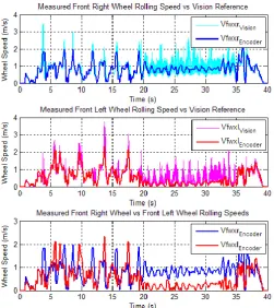
The front wheel rolling speeds obtained from the encoder data can be compared with the global position-based references as shown in Fig. 10. The encoder-based and the vision-based wheel longitudinal speeds of the front right and the front left wheels are compared in the first and the second plots respectively. In addition, the encoder-based wheel rolling speed of the both front wheels are compared to each other in the third plot. Consider the first and the second plots of Fig. 10; the vision-based front wheel longitudinal speeds can be approximated by the encoder-based front wheel rolling speeds. Hence, the assumption of free-rolling front wheels without longitudinal slips is acceptable. In addition, the both front wheel longitudinal speeds are measurable.

Consider the comparison between the encoder-based wheel rolling speeds of the both front wheels, in the third plot of Fig. 10; the wheel rolling speeds correspond to the driving pattern. Generally, the wheel rolling speed of the front right wheel is higher than that of the front left wheel during the positive yaw rate in the CCW rotation; on the contrary, the wheel rolling speed of the front left wheel is higher than that of the front right wheel during the negative yaw rate in the CW rotation. Therefore, the front right wheel rolling speed was sometimes higher than and was sometimes lower than the front left wheel rolling speeds during the 8-figure liked maneuver in the first 20 seconds of the test. On the other hand, the front right wheel rolling speed was always higher than the front left wheel rolling speed during the doughnut maneuver since the 20th _{second to the end of the test.}

The longitudinal and the lateral accelerations measured from the installed on-vehicle inertial measurement unit (IMU) can be compared with the global position-based references as shown in Fig. 11. The IMU-based and the vision-based longitudinal accelerations are shown in the first plot whereas the both lateral accelerations are shown in the second plot. Consider the both plots of Fig. 11; the vision-based references of longitudinal and lateral accelerations can be approximated by the IMU-based longitudinal and lateral accelerations respectively. Hence, the both linear accelerations can be assumed to be measurable for the wheel slip angle estimation.

longitudinal acceleration changed its magnitude and direction in a narrow range between -3 and 3 meters-per-second-squared. The lateral acceleration also changed its magnitude and direction corresponding to the apparently switching of the vehicle yaw rate between the CW and CCW rotations. With large angle of sideslip during the CCW doughnut maneuver in the last 20 seconds of the test, the longitudinal acceleration was the major acceleration component which is the result of the normal acceleration directing toward the ICZV. The magnitude of the longitudinal acceleration was about 4 to 6 meters-per-second-squared pointing to the vehicle heading direction whereas the magnitude of the lateral acceleration was only 1 to 2 meters-per-second-squared pointing to the left of the vehicle.

Fig. 10. The encoder-based front wheel rolling speeds and the vision-based references.

Fig. 11. The IMU-based longitudinal and lateral accelerations and the vision-based references.

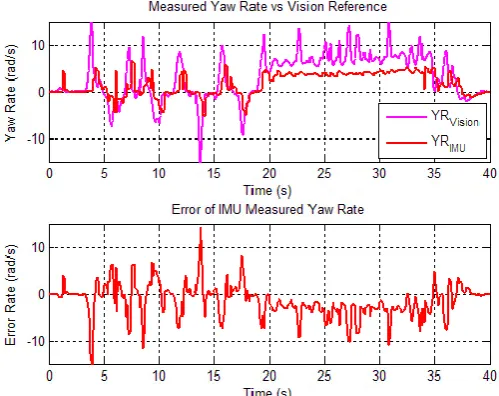
second plot of the same figure. Considering the first plot, the trend of the yaw rate change could be roughly approximated by the IMU measurement. However, significant error of magnitude due to the sensor quality still appeared as can ostensibly be seen in the second plot. The use of the IMU measured yaw rate for the wheel slip angle estimation may cause some significant error in this study. Higher quality gyroscope and appropriate filter for the yaw rate measurement is highly recommended for the further development of this estimation methodology.

Consider the yaw rate plot in Fig. 12 comparing with the steering angle and the sideslip plots in Fig. 9; the variation of yaw rate corresponds to the driving pattern of the testing vehicle as previously mentioned in the discussion of the sideslip and the steering angle. During the test, the vehicle always rotated to respond the steering angle control input. With high speed maneuver, the vehicle sideslip was always in the opposite direction of the yaw rate. Since the yaw rate is positive in the CCW direction whereas the sideslip is positive in the CW direction, it can be clearly noticed about the concordance between the both plots. At the beginning of the test, the vehicle started rotating with the positive yaw rate in the CCW direction to response the negative steering angle in the CCW direction at low very low speed. During the 8-figure liked maneuver from the 3rd _{second to the 18}th _{second, the yaw rate was also switched between the CW and the} CCW directions to respond the steering angle. During the doughnut maneuver from the 18th _{second to} about the 37th _{second, only positive yaw rate appeared in the continuously CCW rotation of the testing} vehicle.

Fig. 12. The IMU-based yaw rate and the vison-based references with their relative error.

By using the proposed kinematics-based analytical closed-form solutions in Eq. (22) and Eq. (23), the individual wheel slip angles of the front right and the front left wheels can be estimated from the on-vehicle measurable information—i.e., the steering angle, the front wheel rolling speeds, the yaw rate, the longitudinal and the lateral accelerations—as plotted comparing with the global position-based references in Fig. 13. The estimated front right wheel slip angle was filtered and compared with its vision reference in the first plot; whereas the estimated front left wheel slip angle was filtered and compared with its vision reference in the second plot. According to the both plots, there are some differences between the filtered wheel slip angles and the vision-based references. The trend of the wheel slip angle changes could be roughly estimated by the proposed estimation methodology. However, significant error of the wheel slip angle magnitudes still appeared during both the 8-figure liked maneuver in the first 20 seconds and the CCW doughnut maneuver in the last 20 seconds of the test. The significant error might considerably be caused by inaccuracy of the yaw rate measurement, as previously mentioned in the above.

wheel in the CCW rotation. On the other hand, the magnitude of the front right wheel slip angle is slightly bigger than that of the front left wheel in the CW rotation of the testing vehicle.

The number of accuracy for this proposed estimation methodology can be evaluated from comparing the filtered wheel slip angles to the vision-based references, as the plots of error angles shown in Fig. 14. For the front right wheel slip angle estimation, the maximum positive error was 59.5 degrees in the CW direction with the average error of 6.3 degrees; whereas, the maximum negative error was 79 degrees in the CCW direction with the average error of 12.6 degrees. For the front left wheel slip angle estimation, the maximum positive error was 75.8 degrees in the CW direction with the average error of 12.6 degrees; whereas, the maximum negative error was 78.7 degrees in the CCW direction with the average error of 11.2 degrees.

Fig. 13. The estimated front wheel slip angles and the vison-based references.

5.

Conclusions

In this paper, the novel cost-effective estimation methodology for all individual wheel slip angle of a RWD vehicle at any slip condition has been proposed. The closed-form solutions of the wheel slip angles written as functions of the on-vehicle measurable information—i.e., the steering angle, the considered wheel rolling speeds, the vehicle yaw rate, the longitudinal and the lateral accelerations—were analyzed from the kinematics of a planar four-wheel vehicle, on the basis of no longitudinal slip at the both front tires. The obtained solutions were primarily verified by computational simulation through an extremely random motion determined by the prescribed functions of the radius of curvature, the vehicle speed, the sideslip and the steering control input. From the simulation, the individual front wheel slip angles could be completely approximated by the developed estimation algorithm with accurate information of the necessary dynamic variables and appropriate switching algorithm. In addition, preliminary implementation was done on the developed 1:10th _{scaled testing vehicle, which was modified so that the steering angle, the front} wheel rolling speeds, the vehicle yaw rate and the linear lateral and longitudinal accelerations could be measured. The testing vehicle was manually controlled to perform extremely random sideslip maneuver beneath the global positioning using four recording cameras. By comparing with the vision-based references, the individual front wheel slip angles could be well approximated despite extreme tire slip in the random maneuver.

Since the proposed wheel slip angle estimation technique was not developed on the basis of kinetic analysis, neither vehicle model nor tire friction model is required for the estimation. In addition, cumulative error due to integration is devoid unlike other kinematics-based estimation techniques. However, appropriate filters to provide accurate information of the required dynamic variables—i.e., the front wheel rolling speeds, the vehicle yaw rate, the longitudinal and the lateral accelerations—are still imperative for the further development of practical applications.

Through direct kinematic relations, the both rear wheel slip angles and the other vehicle state variables—i.e., the radius of curvature, the vehicle sideslip and the vehicle speed—can be also conveniently obtained. Therefore, this proposed estimation methodology could then be alternatively applied for the full range slip angle estimation and the state estimation in advanced active stability control applications dealing with extreme tire slip.

Acknowledgement

This research was partly funded by the Junior Science Talent Project (JSTP) and the Department of Mechanical Engineering, Chulalongkorn University.

References

[1] H. E. Tseng, D. Madau, B. Ashrafi, T. Brown, and D. Recker, “The development of vehicle stability control at Ford,” IEEE/ASME Transactions of Mechatronics, vol. 4, no. 3, pp. 223–234, 1999.

[2] A. T. Van Zanten, “Bosch ESP systems: 5 years of experience,” SAE Transactions, vol. 109, no. 7, pp. 428–436, SAE-Paper 2000-01-1633, 2000.

[3] A. T. Van Zanten, R. Erhardt, G. Pfaff, F. Kost, U. Hartmann, and T. Ehret, “Control aspects of the Bosch-VDC,” in Proceedings of the International Symposium on Advanced Vehicle Control (AVEC’96), Jun. 1996, pp. 573–607.

[4] S. Kimbrough, “Coordinate braking and steering control for emergency stops and accelerations,” in

Proceedings of the WAM ASME, Atlanta, GA, 1991, pp. 229–224.

[5] A. T. Van Zanten, “Evolution of electronic control systems for improving the vehicle dynamic behavior,” in Proceedings of the International Symposium on Advanced Vehicle Control (AVEC’02), 2002, pp. 7-15.

[6] C. R. Carlson, J. C. Gerdes, and D. Powell, “Practical position and yaw rate estimation with GPS and differential wheelspeeds” in Proceedings of the 6th International Symposium of Advanced Vehicle Control (AVEC’02), 2002.

[8] R. M. Rogers, “Improved heading using dual speed sensors for angular rate and odometry in land navigation,” in Proceedings of the Institute of Navigation National Technology Meeting, 1999, pp. 353–361. [9] R. Rajamani, “Lateral vehicle dynamics,” in Vehicle Dynamics and Control. New York: Springer-Verlag,

2005, ch. 2, pp. 15–49.

[10] S. Mammar and D. Koenig, “Vehicle handling improvement by active steering,” Vehicle System Dynamics, vol. 38, pp. 211–242, 2002.

[11] A. Masato, K. Yoshio, S. Kazuasa, S. Yasuji, and F. Yoshimi, “Side-slip control to stabilize vehicle lateral motion by direct yaw moment,” JSAE Review, vol. 22, pp. 413–419, 2001.

[12] J. S. Jo, S. H. You, J. Y. Joeng, K. Y. Lee, and K. Yi, “Vehicle stability control system for enhancing steerability lateral stability, and roll stability,” International Journal of Automotive Technology, vol. 9, no. 5, pp. 571–576, 2008.

[13] P. Heide, R. Schubert, V. Magori, and R. Schwarte, “24 GHz low-cost Doppler speed-over-ground sensor with fundamental-frequency PHEMT-DRO,” in Proceedings of the Gallium Arsenide Application Symposium (GASS’94), Turin, Italy, April, 1994, pp. 233–236.

[14] C. Xu, L. Daniel, E. Hoare, V. Sizov, and M. Cherniakov, “Comparison of speed over ground estimation using acoustic and radar Doppler sensors,” in Proceedings of the European Radar Conference (EuMA’14), Rome, Italy, Oct, 2014, pp. 189–192.

[15] R. Anderson and D. M. Bevly, “Estimation of slip angles using a model based estimator and GPS,” in

Proceedings of the American Control Conference (ACC’04), Boston, MA, Jun, 2004, pp. 2122–2127.

[16] D. M. Bevly, J. Ryu, and J. C. Gerdes, “Integrating INS sensors with GPS measurements for continuous estimation of vehicle sideslip, roll, and tire cornering stiffness” IEEE Transaction on Intelligent Transportation Systems, vol. 7, no. 4, pp. 483–493, 2006.

[17] D. M. Bevly, J. C. Gerdes, C. Wilson, and G. Zhang, “The use of GPS based velocity measurements for improved vehicle state estimation,” in Proceedings of the American Control Conference (ACC’2000), Chicago, IL, Jun, 2000.

[18] D. M. Bevly, R. Sheridan, and J. C. Gerdes, “Integrating INS sensors with GPS velocity measurements for continuous estimation of vehicle sideslip and tire cornering stiffness,” in Proceedings of the American Control Conference (ACC’01), USA, 2001.

[19] J. Ryu, E. J. Rossetter, and J. C. Gerdes, “Vehicle sideslip and roll parameter estimation using GPS,” in Proceedings of the 6th International Symposium of Advanced Vehicle Control (AVEC’2002), 2002.

[20] R. Daily and D. M. Bevly, “The use of GPS for vehicle stability control systems,” IEEE Transactions on Industrial Electronics, vol. 51, no. 2, pp. 270–277, 2004.

[21] J. Farrelly and P. Wellstead, “Estimation of vehicle lateral velocity,” in Proceedings of the IEEE International Conference on Control Applications, Dearborn, MI, Sept., 1996, pp. 552–557.

[22] K. Park, S. J. Heo, and I. Baek, “Controller design for improving lateral vehicle dynamic stability,”

JSAE Review, vol. 22, pp. 481–486, 2001.

[23] B. C. Chen and F. C. Hsieh, “Sideslip angle estimation using extended Kalman filter,” Vehicle System Dynamics, vol. 46, Supplement, pp. 353–364, 2008.

[24] T. Hiraoka, H. Kumamoto, and O. Nishihara, “Sideslip angle estimation and active front steering system based on lateral acceleration data at centers of percussion with respect to front/rear wheels,”

JSAE Review, vol. 25, pp. 37–42, 2004.

[25] J. Stephant, A. Charara, and D. Meizel, “Virtual sensor: application to vehicle sideslip angle and transversal forces,” IEEE Transactions on Industrial Electronics, vol. 51, no. 2, pp. 278–289, 2004.

[26] C. Liu and H. Peng, “A state and parameter identification scheme for linearly parameterized systems,”

ASME Journal of Dynamic System, Measurement, and Control, vol. 120, no. 4, pp. 524–528, 1998.

[27] J. Zuurbier and P. Bremmer, “State estimation for integrated vehicle dynamics control,” in Proceedings of the International Symposium on Advanced Vehicle Control (AVEC’02), Hiroshima, Japan, 2002.

[28] W. Wang, L. Yuan, S. Tao, W. Zhang, and T. Su, “Estimation of vehicle side slip angle in nonlinear condition based on the state feedback observer,” in Proceedings of the IEEE International Conference on Automation and Logistics, Hong Kong and Macau, Aug, 2010, pp. 632–636.

[29] U. Kiencke and A. Daiss, “Observation of lateral vehicle dynamics,” in Proceedings of the International Federation of Automatic Control (IFAC’1996), 1996, pp. 7–10.

[30] A. Hac and M. D. Simpson, “Estimation of vehicle side slip angle and yaw rate,” SAE-Paper 2000-10-0696, 2000.

[32] M. Milanese, D. Regruto, and A. Fortina, “Direct virtual sensor (DVS) design in vehicle sideslip angle estimation” in Proceedings of the American Control Conference (ACC’07), NY, 2007, pp. 3654–3658.

[33] G. Phanomchoeng, R. Rajamani, and D. Piyabongkarn, “Nonlinear observer for bounded Jacobian systems, with applications to automotive slip angle estimation,” IEEE Transactions on Automatic Control, vol. 56, no. 5, pp. 1163–1170, 2011.

[34] T. Zhu and H. Zheng, “Vehicle state estimation based on unscented Kalman state estimation,” in

Proceedings of the International Symposium on Computational Intel, 2008.

[35] Y. Fukada, “Slip-angle estimation for vehicle stability control,” Vehicle System Dynamics, vol. 32, no. 4–5, pp. 375–388, 1999.

[36] A. Nishio, K. Tozu, H. Yamaguchi, K. Asano, and Y. Amano, “Development of vehicle stability control system based on vehicle side slip angle estimation,” SAE-Paper 2001-01-0137, 2001.

[37] D. Piyabongkarn, R. Rajamani, J. A. Grogg, and J. Y. Lew, “Development and experimental evaluation of a slip angle estimator for vehicle stability control,” in Proceedings of the American Control Conference (ACC’06), Minneapolis, MN, Jun, 2006, pp. 5366–5371.

[38] F. Cheli, E. Sabbioni, M. Pesce, and S. Melzi, “A methodology for vehicle sideslip angle identification: comparison with experimental data,” Vehicle System Dynamics, vol. 45, no. 6, pp. 549–563, 2007.

[39] T. Iijima, P. Raksincharoensak, Y. Michitsuji, and M. Nagai, “Vehicle side slip angle estimation methodology using a drive recorder,” Journal of Vibration and Control, vol. 16, no. 4, pp. 571–583, 2010. [40] M. Shang, L. Chu, J. Guo, and Y. Fang, “Estimation of vehicle side slip Angle using hybrid observer,”

in Proceedings of the Chinese Control Conference (CCC’10), Beijing, China, Jul, 2010, pp. 5378–5383.

[41] D. W. Pi, N. Chen, J. X. Wang, and B. J. Zhang, “Design and evaluation of sideslip angle observer for vehicle stability control,” International Journal of Automotive Technology, vol. 12, no. 3, pp. 391–399, 2011. [42] K. Hsu, M. Milanese, C. Novara, and K. Poolla, “Nonlinear virtual sensors design from data,” in

Proceedings of the IFAC Symposium on System Identification (SYSID’06), Newcastle, Australia, 2006.

[43] M. Milanese, C. Novara, K. Hsu, and K. Poolla, “Filter design from data: direct vs. two-step approaches,” in Proceedings of the American Control Conference (ACC’06), Minneapolis, MN, Jun. 2006. [44] R. Chaichaowarat and W. Wannasuphoprasit, “Optimal control for steady state drifting of RWD

vehicle,” in Proceedings of the 7th IFAC Symposium on Advances in Automotive Control (IFAC-AAC’ 2013), Tokyo, Japan, 2013, pp. 814–820.

[45] R. Chaichaowarat and W. Wannasuphoprasit, “Two dimensional dynamic model of drifting vehicle,” in Proceedings of the 7th International Conference on Automotive Engineering (ICAE-7), Bangkok, Thailand, 2011.