Communications Engineering Laboratory of Electromechanics
Teknillinen korkeakoulu sähkö- ja tietoliikennetekniikan osasto sähkömekaniikan laboratorio
Espoo 2000 Raportti 63
INDUCTION MOTOR MODELLING FOR
VECTOR CONTROL PURPOSES
Mircea Popescu
Helsinki University of Technology
Department of Electrical and Communications Engineering Laboratory of Electromechanics
Teknillinen korkeakoulu
Sähkö- ja tietoliikennetekniikan osasto Sähkömekaniikan laboratorio
Popescu M., Induction Motor Modelling for Vector Control Purposes, Helsinki University of Technology, Laboratory of Electromechanics, Report, Espoo 2000, 144 p.
Keywords: Induction motor, vector control, d-q models, continuos time domain, discrete time domain, linearization
Abstract
Widely used in many industrial applications, the induction motors represent the starting point when an electrical drive system has to be designed. In modern control theory, the induction motor is described by different mathematical models, according to the employed control method. In the symmetrical three-phase version or in the unsymmetrical two-phase version, this electrical motor type can be associated with vector control strategy. Through this control method, the induction motor operation can be analysed in a similar way to a DC motor. The goal of this research is to summarize the existing models and to develop new models, in order to obtain a unified approach on modelling of the induction machines for vector control purposes. Starting from vector control principles, the work suggests the d-q axes unified approach for all types of the induction motors. However, the space vector analysis is presented as a strong tool in modelling of the symmetrical induction machines. When an electrical motor is viewed as a mathematical system, with inputs and outputs, it can be analysed and described in multiple ways, considering different reference frames and state-space variables. All the mathematical possible models are illustrated in this report. The suggestions for what model is suitable for what application, are defined as well. As the practical implementation of the vector control strategies require digital signal processors (DSP), from the continuos time domain models are derived the discrete time domain models. The discrete models permit the implementation of the mathematical model of the induction motors, in order to obtain high efficiency sensorless drives. The stability of these various models is analysed.
Distribution:
Helsinki University of Technology Laboratory of Electromechanics P.O. Box 3000 FIN-02015 HUT Tel: +358-9-451-2384 Fax: +358-9-451-2991 E-mail: [email protected] © Mircea Popescu ISBN 951-22-5219-8 ISSN 1456-6001 Picaset Oy Helsinki 2000
Contens
Abstract ……….……….… Preface ………..….. List of principal symbols ……….………..……. 1. Vector control of induction motors - Overview………..…………...
1.1 Introduction ………
1.2 Algorithm of Vector Control ………..
1.3 Field Orientation Control ………
1.4 Direct Torque Control ………
2. Continous-time domain linear models of the three-phase induction machine …………..
2.1 Introduction ………
2.2 Voltage and flux linkage equations ……… 2.3 Space vector equations for three-phase induction machines ……….. 2.4 Vectorial equations system in a common reference frame ……….…… 2.5 Induction machine equations with stator referred rotor variables ………….. 2.6 Instantaneous electromagnetic torque ……… 2.7 General equations of the induction machine in different reference frames ….
2.7.1. Per unit system ………. 2.7.2. Stationary reference frame equations. Block diagram ……….. 2.7.3. Rotor reference frame. Block diagram ………. 2.7.4. Synchronous reference frame. Block diagram ………. 2.8. D-Q Axes models of the three-phase induction machine ………... 2.8.1. Models with currents space vectors as state-space variables …………... 2.8.2. Models with fluxes linkages space vectors as state-space variables …… 2.8.3. Models with mixed currents -flux space vectors as state-space variables 2.9. Vector control strategies for three-phase induction machine ……….
2.9.1. Stator flux field orientation (SFO) ……… 2.9.2. Rotor flux field orientation (RFO) ……… 2.9.3. Air-gap flux field orientation (AFO) ……… 2.9.4. Stator current orientation (SCO) ……….. 2.9.5. Rotor current orientation (RCO) ………... 3. Continuos-time domain models of the single-phase induction machine ………
3.1. Introduction ………
3.2. Voltage and flux-current equations of the single-phase induction machine .. 3.3. Analysis of the single-phase induction machine in stationary reference
frame ………... 3.4. Analysis of the steady-state operation for the symmetrical single-phase induction machine ……….. 3.5. Analysis of the unsymmetrical single-phase induction machine ……… 3.6. Continuos linear models for single-phase induction machine ……… 3.6.1. LinearΓ model of the symmetrical single-phase induction machine .
2 3 6 9 9 11 13 14 17 17 17 21 24 26 27 29 29 31 32 34 41 43 45 47 51 52 54 56 58 60 65 65 65 68 70 71 72 73
3.6.2. Linear inverse Γ model of the symmetrical single-phase induction machine ……….. 3.6.3. Universal model of the symmetrical single-phase induction machine 3.6.4. Linear Γ model of the unsymmetrical single-phase induction
machine ……….. 3.6.5. Linear inverse Γ model of the unsymmetrical single-phase induction
machine ………... 3.6.6. Universal model of the unsymmetrical single-phase induction
machine ……….. 3.7. D-Q axes models of the single-phase induction machine ……….. 3.7.1. Models with currents space vectors as state-space variables ………. 3.7.2. Models with fluxes linkages space vectors as state-space variables .. 3.7.3. Models with mixed currents-fluxes space vectors as state-space
variables ……….. 3.8. Vector control strategies for single-phase induction machine ……… 3.8.1. Stator flux field orientation (SFO) ………. 3.8.2. Rotor flux field orientation (RFO) ………. 3.8.3. Air-gap flux field orientation (AFO) ……….. 3.8.4. Stator current orientation (SCO) ……… 3.8.5. Rotor current orientation (RCO) ……… 4. Mathematical discrete models for the three-phase induction machine ………..
4.1. Introduction ………..………..
4.2. Bilinear transformation method (Tustin) ……… 4.3. Forward-differences method (Euler) ………..
4.4. Backward-differences method ………
4.5. Z-domain transfer functions ………
4.6. Stability analysis ……….
5. Mathematical discrete models for the single-phase induction machine ……….
5.1. Introduction ……….
5.2. Bilinear transformation method (Tustin) ……… 5.3. Forward-differences method (Euler) ………..
5.4. Backward-differences method ………
5.5. Z-domain transfer functions ………
6. Linearisation of the induction machine mathematical models ………...
6.1. Introduction ………
6.2. Three-phase induction machine ……….
6.3. Single-phase induction machine ………
References ……….. 74 76 78 79 81 83 84 87 89 94 95 97 99 101 104 108 108 110 113 115 117 121 123 123 125 127 129 131 135 135 136 138 141
List of principal symbols:
Scalar variables are denoted by plane letters. Vector variables are denoted by underlined letters. Boldface symbols are used for matrix variables.
, , , , ,
A B C D E F state-space coefficient matrix ij
a coefficients for state-space variables m
B viscous friction coefficient
H relative inertia constant
H transfer function matrix
(a,b,c)s
I instantaneous stator phase current for the three-phase induction machine (a,b,c)r
I instantaneous rotor phase current for the three-phase induction machine (d,q)s
I
ɶ complex stator phase currents in d-q co-ordinates for steady-state analysis (a,b)s
I
ɶ complex stator phase currents in physical co-ordinates for steady-state analysis
(d,q)r I
ɶ complex rotor phase currents in d-q co-ordinates for steady-state analysis (a,b)r
I
ɶ complex rotor phase currents in physical co-ordinates for steady-state analysis
s
I stator current space vector
r
I rotor current space vector
(a,b,c)s
i instantaneous stator phase currents for the three-phase induction machine (a,b,c)r
i instantaneous rotor phase currents for the three-phase induction machine (a,b)s
i instantaneous stator phase currents for the single-phase induction machine (a,b)r
i instantaneous rotor phase currents for the single-phase induction machine (A,B,C)s
i phase currents for a three-phase system (X,Y)s
i phase currents for an orthogonal two-phase system (d,q)s
i instantaneous stator phase currents in d-q co-ordinates (d,q)r
'
i instantaneous referred rotor phase currents in d-q co-ordinates (d,q)R
'
i Γ models instantaneous referred rotor phase currents in d-q co-ordinates s( , )R I
i stator phase currents in complex co-ordinates and per unit system r ( , )
' R I
i rotor phase currents in complex co-ordinates and per unit system s
i stator current space vector in per unit system r
'
i referred rotor current space vector in per unit system
J inertia constant
j complex operator
p,i
K proportional, respectively integrative constant for PI controllers s,r
s,r
K transformation matrix from abcco-ordinates to d-q co-ordinates k turns ratio for the unsymmetrical single-phase machine
(a,b,c)(s,r)
l(s,r)
L leakage inductance for symmetrical stator phase, respectively rotor l(m,a)
L leakage inductance for unsymmetrical stator phase: main, respectively auxiliary
M
l magnetisation inductance in per unit system s
l total stator inductance in per unit system r
'
l total rotor inductance in per unit system (a,b,c),(s,r)
M mutual inductance for stator phase, respectively rotor s,r
N turns number for stator phase, respectively rotor
P number of poles
p derivative operator
s
R per unit stator phase resistance for the three-phase induction machine s
r stator phase resistance for the symmetrical induction machine m
r main stator phase resistance for the unsymmetrical single-phase machine a
r auxiliary stator phase resistance for the unsymmetrical single-phase machine r
r rotor phase resistance for the symmetrical induction machine r
'
r referred rotor phase resistance for the symmetrical induction machine
s Laplace operator
m
s critical slip for the induction machine
T sampling period
e
T instantaneous electromagnetic torque
L
T load torque
t time
(a,b,c)s
U instantaneous stator phase voltage for the three-phase induction machine (a,b,c)r
U instantaneous rotor phase voltage for the three-phase induction machine s ( , )R I
U stator phase voltage in complex co-ordinates and per unit system °(d,q)s
U complex stator phase voltages in d-q co-ordinates for steady-state analysis °(a,b)s
U complex stator phase voltages in physical co-ordinates for steady-state analysis
s
U stator voltage space vector
r
U rotor voltage space vector
(d,q)s
u instantaneous stator phase voltages in d-q co-ordinates (d,q)r
'
u instantaneous rotor phase voltages in d-q co-ordinates s
u stator voltage space vector in per unit system r
'
u referred rotor voltage space vector in per unit system c
W magnetic coenergy
b
X base variable value for per unit system
x space vector variable
m
x magnetisation reactance
ls
l(m,a)
x stator phase leakage reactance for the unsymmetrical induction machine: main, respectively auxiliary
lr
'
x rotor leakage reactance
L
x Γ models equivalent leakage reactance for symmetrical induction machine L(d,q)
x Γ models equivalent leakage reactance for unsymmetrical induction machine M
x Γ models equivalent magnetisation reactance for symmetrical induction machine
M(d,q)
x Γ models equivalent magnetisation reactance for unsymmetrical induction machine
z discrete co-ordinate
α space vector operator
γ Γ models turns ratio for symmetrical induction machine (d,q)
γ Γ models turns ratio for unsymmetrical induction machine ,
R I
∆ real, respectively imaginary component of a matrix determinant (d,q)s
ψ stator flux linkage ind-q co-ordinates and per unit system (d,q)m
ψ magnetisating flux linkage in d-q co-ordinates and per unit system (d,q)r
ψ rotor flux linkage in d-q co-ordinates and per unit system s( , )R I
ψ stator flux linkage in complex co-ordinates and per unit system r( , )
' R I
ψ rotor flux linkage in complex co-ordinates and per unit system (d,q)s
λ stator flux linkage in d-q co-ordinates and flux linkage units per second. (a,b,c)s
λ stator flux linkage fluxes in abs or ab co-ordinates (d,q)r
'
λ referred rotor linkage fluxes in d-q co-ordinates and flux linkage units per second
(d,q)R '
λ Γ models referred rotor linkage fluxes in d-q co-ordinates and flux linkage units per second
(a,b,c)r
λ rotor flux linkage in abs or ab co-ordinates r
'
λ referred rotor flux linkage space vector for three-phase induction machine s
λ stator flux linkage space vector for three-phase induction machine
γ
λ arbitrarily flux linkage space vector for three-phase induction machine m
ℜ magnetic reluctance
s,r
σ leakage factor for stator phase, respectively rotor phase r
θ periferical displacement between stator and rotor space vectors k
θ periferical displacement between stator and arbitrary space vectors
Ω relative angular frequency in per unit system
ω angular frequency of the supply system
b
ω base angular frequency of the supply system n
ω rated angular frequency of the induction machine in electrical degrees r
1. VECTOR CONTROL OF INDUCTION MOTORS - OVERVIEW
1.1.Introduction
The electrical DC drive systems are still used in a wide range of industrial applications, although they are less reliable than the AC drives. Their advantage consists in simple and precise command and control structures.
The AC drives, sometimes more expensive but far more reliable, (Rajashekara et al. 1996) require complex modern control techniques. The design of a control system is realised in two important steps:
1. The drive system has to be converted into a mathematical model, in order to accomplish the analysis and the evaluation of the system.
2. The imposed response of the drive system is obtained through an optimal regulator, when external perturbations are present.
The induction motors are relatively cheap and rugged machines because their construction is realised without slip rings or commutators. These advantages have determined an important development of the electrical drives, with induction machine as the execution element, for all related aspects: starting, braking, speed reversal, speed change, etc. The dynamic operation of the induction machine drive system has an important role on the overall performance of the system of which it is a part.
There are two fundamental directions for the induction motor control:
• Analogue: direct measurement of the machine parameters (mainly the rotor speed), which are compared to the reference signals through closed control loops;
• Digital: estimation of the machine parameters in the sensorless control schemes (without measuring the rotor speed), with the following implementation methodologies:
• Slip frequency calculation method; • Speed estimation using state equation;
• Estimation based on slot space harmonic voltages; • Flux estimation and flux vector control;
• Direct control of torque and flux;
• Observer-based speed sensorless control; • Model reference adaptive systems; • Kalman filtering techniques;
• Sensorless control with parameter adaptation; • Neural network based sensorless control; • Fuzzy-logic based sensorless control.
Another classification of the control techniques for the induction machine is made by Holtz (1998) from the point of view of the controlled signal:
a) Scalar control:
a.1 Voltage/frequency (or v/f) control;
a.2 Stator current control and slip frequency control. These techniques are mainly implemented through direct measurement of the machine parameters.
b) Vector control:
b.1 Field orientation control (FOC): b.1.1. Indirect method; b.1.2. Direct method;
b.2 Direct torque and stator flux vector control. These techniques are realised both in analogue version (direct measurements) and digital version (estimation techniques)
The development of accurate system models is fundamental to each stage in the design, analysis and control of all electrical machines. The level of precision required of these models depends entirely on the design stage under consideration. In particular, the mathematical description used in
machine design requires very fine tolerance levels as stated by Nabae et al. (1980) and Murata et al (1990). However, in the development of suitable models for control purposes, it is possible to make certain assumptions that considerably simplify the resulting machine model. Nonetheless, these models must incorporate the essential elements of both the electromagnetic and the mechanical systems for both steady state and transient operating conditions (Nowotny and Lipo - 1996). Additionally, since modern electric machines are invariably fed from switching power conversion stages, the developed motor models should be valid for arbitrary applied voltage and current waveforms. This work presents suitable models for use in digital current control of the induction motors. In addition, the limits of the validity of these models are summarised and, in some cases, the models are extended to account for some non-idealities of the machine.
Usually, the following assumptions are made (Lorenz et al. 1994):
• No magnetic saturation, i.e. machine inductance is not affected by current level. • No saliency effects i.e. machine inductance are not functions of position.
• Negligible spatial mmf harmonics i.e. stator windings are arranged to produce sinusoidal mmf distributions.
• The effects of the stator slots may be neglected. • There is no fringing of the magnetic circuit.
• The magnetic field intensity is constant and radially directed across the air-gap. • Eddy current and hysteresis effects are negligible.
The modern control theory for an electrical drive system requires the existence of a real-time, stabile, and precise mathematical model for each component of the system. The analysis and the design of the numerical command for such systems depend on the hardware and software resources. If in communication techniques the real-time response of the system is not always compulsory, in industrial processes the real-time response of the drive systems is essential.
The soft numerical command for the electrical drive systems is far more flexible to implement than the hardware version. For the latter, lately there is an intense research effort for implementing ASIC (application specific integrated circuit). The numerical command of the electrical drive systems is a challenging task mainly due to the DSP (digital signal processing) technology. Now it is possible to realise linear and non-linear techniques for implementing continuos and discrete mathematical models of the entire element of an electrical drive system, including the electrical machine (Xu and Nowotny - 1990, 1992).
For the AC drives there are several solutions for implementing the command and the control of the system. A quick summary of the existing technologies already out there in the field is given below:
DC Drives
Initially the DC drives were used for variable speed control because they could easily achieve a good torque and speed response with high accuracy. Field orientation of the motor is achieved using a mechanical commutator with brushes. In DC, torque is controlled using the armature current and field current. The main drawback of this technique is the reduced reliability of the DC motor - the fact that brushes and commutators wear down and need regular servicing; that DC motors can be costly to purchase; and that they require encoders for positional feedback.
AC Drives
The evolution of AC variable speed drive technology has been partly driven by the desire to emulate the performance of the DC drive, such as fast torque response and speed accuracy, while using robust, cheap to purchase and relatively maintenancefree AC motors (Kelemen and Imecs -1987).
AC Drives, frequency controlled using PWM
With this technique, sometimes known as scalar control, the field orientation of the motor is not used. Instead, the frequency and the voltage are the main control variables and are applied to the stator windings. The status of the rotor is ignored, meaning that no speed or position signal is fed
back. The drive is therefore regarded as an open-loop drive. This type of drive is suitable for applications such as pumps and fans, which do not require high levels of accuracy or precision. AC Drives, flux vector control using PWM
Here, field orientation is achieved by mathematical modelling using microprocessors and feedback of rotor speed and angular position relative to the stator field by means of an encoder (Vas - 1990). This results in a drive with greater stability and capable of fast torque response and accurate speed control. But the drawback is the need for the encoder, which reduces drive system reliability and adds cost. The controlling variables in a DC drive for torque are armature current and field current, and armature voltage for torque. AC drives using the PWM principle; however, use voltage and frequency as the controlling variables and these are controlled by a device called a modulator. A modulator adds considerable delay in the responsiveness of a motor to changes in torque and speed. Furthermore, with flux vector AC drives, a tacho-generator or position encoder is invariably needed to obtain any real degree of accuracy. Such devices are costly and compromise the simplicity of the AC induction motor.
AC Drives, sensorless flux vector
The flux vector controlled drive with encoder feedback does offer very high levels of performance across a wide power range and should not be confused with sensorless vector - or open loop vector - drives, which offer performance only slightly superior to that of a standard inverter using scalar control (Rajashekara et al. - 1996).
1.2.Algorithm of vector control
The induction motors are very common because they are inexpensive and robust, finding use in everything from industrial applications such as pumps, fans, and blowers to home appliances. Traditionally, induction motors have been run at a single speed, which was determined by the frequency of the main voltage and the number of poles in the motor. Controlling the speed of an induction motor is far more difficult than controlling the speed of a DC motor since there is no linear relationship between the motor current and the resulting torque as there is for a DC motor.
The technique called vector control can be used to vary the speed of an induction motor over a wide range. It was initially developed by Blaschke (1971-1973). In the vector control scheme, a complex current is synthesised from two quadrature components, one of which is responsible for the flux level in the motor, and another which controls the torque production in the motor. Essentially, the control problem is reformulated to resemble the control of a DC motor. Vector control offers a number of benefits including speed control over a wide range, precise speed regulation, fast dynamic response, and operation above base speed.
The vector control algorithm is based on two fundamental ideas. The first is the flux and torque producing currents. An induction motor can be modelled most simply (and controlled most simply) using two quadrature currents rather than the familiar three phase currents actually applied to the motor. These two currents called direct (Id) and quadrature (Iq) are responsible for producing flux
and torque respectively in the motor. By definition, the Iq current is in phase with the stator flux,
and Id is at right angles. Of course, the actual voltages applied to the motor and the resulting
currents are in the familiar three-phase system. The move between a stationary reference frame and a reference frame, which is rotating synchronous with the stator flux, becomes then the problem. This leads to the second fundamental idea behind vector control.
The second fundamental idea is that of reference frames. The idea of a reference frame is to transform a quantity that is sinusoidal in one reference frame, to a constant value in a reference frame, which is rotating at the same frequency. Once a sinusoidal quantity is transformed to a constant value by careful choice of reference frame, it becomes possible to control that quantity with traditional proportional integral (PI) controllers.
Vector transforms
The Park and Clarke vector transforms are one of the keys to vector control of induction motors. I) Clarke transform
The forward Clarke (1943) transform does a magnitude invariant translation from a three phase system into two orthogonal components. If the neutral - ground connection is neglected, the variables in a three-phase system (A, B, and C) sum is equal to zero, and there is a redundant information. Therefore, the system can be reduced to two variables, called X and Y. The Clarke transform is given by:
As Xs Bs Ys Cs ( ) ( ) 2 1 cos( ) cos(2 ) ( ) ( ) 3 0 sin( ) sin(2 ) ( ) i t i t i t i t i t γ γ γ γ = ⋅ ⋅ (1) where: 2 3
π
γ
=Using the relation:
As( ) Bs( ) Cs( ) 0
i t +i t +i t = (2) and the fact that:
2 4 1 c o s c o s 3 3 2 π π = = − (3) Thus, the Clarke transform can be simplified to:
(
)
As X s As C s B s ( ) ( ) 1 ( ) ( ) ( ) 3 i t i t i t i t i t = ⋅ − (4) The Clarke transform can also be understood using a vector diagram as shown in Fig. 1.1. In the figure, A, B, and C are the axes of a three phase system, each offset 120° from the other. X and Y are the axes of a two variable system where X is chosen to be coincident with A. To perform the Clarke transform of a three variable system (iA, iB, iC), iX is equal to iA and iY is the scaledprojection of iB and iC onto the Y axis. The scaling is necessary to preserve the signal magnitudes
through the transform.
B Y i C A, X 0 iX iB iC i Y s i A =
Fig. 1.1. Clarke Transform Vector Diagram
The Clarke transform preserves the magnitude, and realise a quadrature between the current components.
II) Park transform
The Park (1929) transform is a vector rotation, which rotates a vector (defined by its quadrature components) through a specified angle. The Park transform function implements the following set of equations: x x y y O u t ( ) cos( ) sin( ) In ( ) O u t ( ) sin( ) cos( ) In ( ) t t t t θ θ θ θ − = ⋅ (5) whereθ is the angle to rotate the vector through. A reverse vector rotation can be accomplished simply by changing the sign on the sin (θ) input value. The vector rotation is illustrated by Fig. 1.2.
Some references (Vas -1990, Nowotny and Lipo - 1996) describe the Park transform as a combination of the Clark and Park transforms presented here. Breaking into a three-variable-to-two transform (i.e. the Clarke transform) and a vector rotation is done for efficiency of calculation: with separate Park and Clarke transforms, only two trigonometric calculations are required as opposed to 6 in the traditional Park transform.
Q Y i D X 0 iX iQ i D iY θ s
Fig.1.2. Park transform vector diagram
1. 3. Field orientation control (FOC)
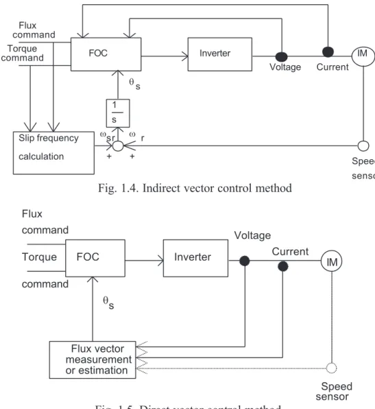
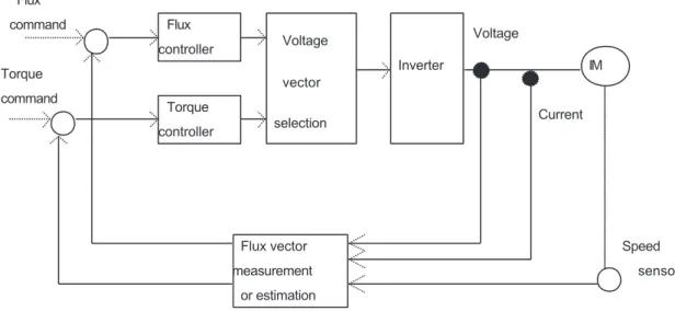
Vector control techniques have made possible the application of induction motors for high-performance applications where traditionally only DC drives were applied (Holtz - 1995). The vector control scheme enables the control of the induction motor in the same way as separately excitation DC motors. As in the DC motor, torque control of induction motor is achieved by controlling the torque current component and flux current component independently. The basic schemes of indirect and direct methods of vector control are shown in Figs. 1.3 –1.5. The direct vector control method depends on the generation of unit vector signals from the stator or air-gap flux signals. The air-gap signals can be measured directly or estimated from the stator voltage and current signals. The stator flux components can be directly computed from stator quantities. In these systems, rotor speed is not required for obtaining rotor field angle information. In the indirect vector control method, the rotor field angle and thus the unit vectors are indirectly obtained by summation of the rotor speed and slip frequency.
Flux
Stator
θs
FOC Inverter IM Speed sensor Slip frequency calculation Flux command Torque command + + Voltage Current ω ωsr r 1 s θs
Fig. 1.4. Indirect vector control method Flux command Torque command FOC Inverter Voltage Current IM Speed sensor Flux vector measurement or estimation θs
Fig. 1.5. Direct vector control method
Fundamental requirements for the FOC are the knowledge of two currents (if the induction motor is star connected) and the rotor flux position. Knowledge of the rotor flux position is the core of the FOC. In fact if there is an error in this variable the rotor flux is not aligned with d-axis and the current components are incorrectly estimated. In the induction machine the rotor speed is not equal to the rotor flux speed (there is a slip speed; as such, a special method to calculate the rotor flux position (angle) is needed. The basic method is the use of the current model.
Thanks to FOC it becomes possible to control, directly and separately, the torque and flux of the induction motors. Field oriented controlled induction machines obtain every DC machine advantage: instantaneous control of the separate quantities allowing accurate transient and steady-state management.
1. 4. Direct torque control
The most modern technique is direct torque and stator flux vector control method (DTC). It has been realised in an industrial way by ABB, by using the theoretical background proposed by Blashke and Depenbrock during 1971-1985. This solution is based both on field oriented control (FOC) as well as on the direct self-control theory.
Starting with a few basics in a variable speed drive the basic function is to control the flow of energy from the mains to a process via the shaft of a motor. Two physical quantities describe the state of the shaft: torque and speed. Controlling the flow of energy depends on controlling these
quantities. In practice either one of them is controlled and we speak of "torque control" or "speed control". When a variable speed drive operates in torque control mode the speed is determined by the load. Torque is a function of the actual current and actual flux in the machine. Likewise when operated in speed control the torque is determined by the load.
Variable speed drives are used in all industries to control precisely the speed of electric motors driving loads ranging from pumps and fans to complex drives on paper machines rolling mills cranes and similar drives.
The idea is that motor flux and torque are used as primary control variables which is contrary to the way in which traditional AC drives control input frequency and voltage, but is in principle similar to what is done with a DC drive, where it is much more straightforward to achieve. In contrast, traditional PWM and flux vector drives use output voltage and output frequency as the primary control variables but these need to be pulse width modulated before being applied to the motor. This modulator stage adds to the signal processing time and therefore limits the level of torque and speed response time possible from the PWM drive.
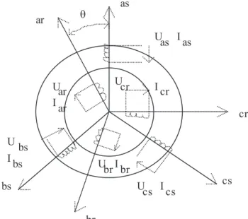
In contrast, by controlling motor torque directly, DTC provides dynamic speed accuracy equivalent to closed loop AC and DC systems and torque response times that are 10 times faster. It is also claimed that the DTC does not generate noise like that produced by conventional PWM AC drives. And the wider spectrum of noise means that amplitudes are lower which helps to control EMI and RFI emissions. The basic structure of direct torque and stator flux vector control is presented in Fig. 1.6. Flux command Torque command Flux controller Torque controller Voltage vector selection Inverter Voltage Current IM Speed sensor Flux vector measurement or estimation
Fig. 1.6. Basic structure of direct torque and flux vector control
In DTC field orientation is achieved without feedback using advanced motor theory to calculate the motor torque directly and stator flux without using a modulator or a requirement for a tachogenerator or position encoder to feed back the speed or position of the motor shaft. Both parameters are obtained instead from the motor itself. DTC's configuration also relies on two key developments - the latest high-speed signal processing technology and a highly advanced motor model precisely simulating the actual motor within the controller. A DSP (digital signal processor) is used together with ASIC hardware to determine the switching logic of the inverter.
The motor model is programmed with information about the motor, which enables it to determine parameters including stator resistance, mutual inductance saturation coefficients and motor inertia. The model also encompasses temperature compensation, which is essential for good static speed accuracy without encoder.
In normal operation, measurements of the two motor phase currents and the drive DC link voltage, together with information about the switching state of the inverter are fed into the motor model . The motor model then outputs control signals, which are accurate estimates of the actual motor torque and actual stator flux. All control signals are transmitted via optical links for high speed. In this way, the semiconductor switching devices of the inverter are supplied with an optimum switching pattern for reaching or maintaining an accurate motor torque.
Also, both shaft speed and electrical frequency are calculated within the motor model. There is no need to feedback any shaft speed or position with tachometers or encoders to meet the demands of 95% of industrial applications. However, there will always be some special applications where even greater speed accuracy will be needed and when the use of an encoder improves the accuracy of speed control in DTC. But even then, the encoder does not need to be as costly or as accurate as the one used in traditional flux vector drives, as DTC only has to know the error in speed, not the rotor position.
The drive will have a torque response time typically better than 5ms. This compares with response for both flux vector PWM drives and DC drives fitted with encoders. The newer sensorless flux vector drives now being launched by other drives manufacturers have a torque response measured in hundreds of milliseconds.
DTC also provides exceptional torque control linearity. For the first time with an open loop AC drive, torque control can be obtained at low frequencies, including zero speed, where the nominal torque step can be increased in less than 1ms. The dynamic speed accuracy of DTC drives is better than any open loop AC drives and comparable to DC drives, which use feedback.
DTC brings other special functions, not previously available with AC drives, including automatic starting in all motor electromagnetic and mechanical states. There is no need for additional parameter adjustments, such as torque boost or starting mode selection, such as flying start. DTC control automatically adapts itself to the required condition. In addition, based on exact and rapid control of the drive intermediate DC link voltage, DTC can withstand sudden load transients caused by the process, without any overvoltage or overcurrent trip.
2. CONTINUOUS-TIME DOMAIN LINEAR MODELS OF THE
THREE-PHASE INDUCTION MACHINE
2.1. Introduction
Until the last decades the three-phase induction machine was mainly used in constant speed drives due to the control system performance, not to the operating principle of the machine.
Nowadays, this situation is completely changed. With the technical progress in power electronics and microelectronics, the three-phase induction machine control becomes very flexible and highly efficient. Since 1983, the year when the digital signal processor (DSP) appeared, the control theory for this type of machine was permanently improved.
New mathematical models have to be implemented for the three-phase induction machine in order to analyse its operation both dynamically and in steady-state.
2.2. Voltage and flux linkage equations
The first mathematical model for the dynamic analysis of the induction machine was based on the two real axis reference frame, developed initially by Park (1929) for the synchronous machine. Using the symmetric configuration of the induction machine, Kovacs and Racz (1959) have elaborated the space complex vector theory, and obtained a model for the steady-state analysis of the machine. Both theories are used for modelling the three-phase induction machine. The following assumptions are made when a complete equations system is written to describe the continuous-time linear model of the induction machine (Krause et al. 1995):
• Geometrical and electrical machine configuration is symmetrical; • Space harmonics of the stator and rotor magnetic flux are negligible; • Infinitely permeable iron;
• Stator and rotor windings are sinusoidally distributed in space and replaced by an equivalent concentrated winding;
• Saliency effects, the slotting effects are neglected;
• Magnetic saturation, anisotropy effect, core loss and skin effect are negligible; • Windings resistance and reactance do not vary with the temperature;
• Currents and voltages are sinusoidal terms. • End and fringing effects are neglected
All these assumptions do not alter in a serious way the final result for a wide range of induction machines.
as cs bs cr ar br Uas Ias U cs Ics U bs I bs Ucr I cr U br I br ar ar U I θ
Fig. 2.1. The real model of the three-phase induction machine with three stator windings and three rotor windings
For the machine stator in Fig.2.1 if we choose the stator reference frame, the voltage equations are as follows: as a s s as bs bs s bs cs c s s cs d U r I dt d U r I dt d U r I dt λ λ λ = + = + = + (6-8)
where Ua s, Ubs, Ucs are the instantaneous stator voltages, Ias, Ibs, Ic s are the instantaneous stator currents, rs = ras = rbs = rcs is the stator winding resistance and λas, λbs, λcsare the total magnetic fluxes for the three stator windings.
The flux-current relations are determined after detailing the total flux of a stator winding. For the other two windings, there are valid similar relations:
as asas bsas csas aras bras cras
λ =λ +λ +λ +λ +λ +λ (9) where the flux components are:
asas
λ the magnetic flux produced by stator phase current as in the stator phase winding as bsas
λ the magnetic flux produced by stator phase current bs in the stator phase winding as csas
λ the magnetic flux produced by stator phase current cs in the stator phase winding as aras
λ the magnetic flux produced by rotor phase current ar in the stator phase winding as bras
λ the magnetic flux produced by rotor phase current br in the stator phase winding as cras
λ the magnetic flux produced by rotor phase current cr in the stator phase winding as These components are computed with the expressions:
asas as as bsas bsas bs csas csas cs L I M I M I λ λ λ = = = aras aras ar bras bras br cras cras cr M I M I M I λ λ λ = = =
Self-inductance Las has two components, one created by the linkage magnetic flux Lmas and the
second created by the leakage magnetic flux Llas: las
mas
as L L
L = + (10) The mutual inductance, which is considered to be equal due to the machine symmetry, can also be split in two components. However, the leakage flux created component in the mutual inductance can be neglected. It results that:
asbs bsas ascs csas mas 1
2
M =M =M = M = − L (11) The mutual inductance within the stator and rotor windings varies with the relative space position between them. The stator flux created by current from rotor phase ar in stator phase as depend on the angle value θ:
2 w 2
aras asar mas mas
s w t 1 cos cos s w k M M L L w k θ k θ = = ⋅ ⋅ = ⋅ ⋅ (12) where kt represents the turn ratio multiplied by the winding factor ratio. In a similar way the
relations for the others mutual inductances can be written: bras asbr mas
t cras ascr mas
t 1 2 cos 3 1 4 cos 3 M M L k M M L k π θ π θ = = ⋅ ⋅ + = = ⋅ ⋅ + (13-14) Due to the symmetrical configuration of the induction machine, we can deduce the total magnetic flux for the stator phase winding as expressed as follows:
(
)
as mas las as mas bs mas cs mas ar t mas br mas cr t t 1 1 1 cos 2 2 1 2 1 4 cos cos 3 3 L L I L I L I L I k L I L I k k λ θ π π θ θ = + ⋅ − ⋅ − ⋅ + ⋅ + ⋅ + + ⋅ + (15)
For the rotor windings, by using a rotor reference frame, it can be developed a similar equation system to the stator case:
ar a r r ar bar br r br cr r cr cr d U r I dt d U r I dt d U r I dt λ λ λ = + = + = + (16-18)
where: Uar,Ubr,Ucr are the instantaneous rotor voltages, Iar,Ibr,Icr are the instantaneous rotor currents, rr = ra r = rbr = rcr is the rotor winding resistance and λ λ λar, br, crare the total magnetic fluxes for the three rotor windings.
The total rotor magnetic flux for the winding ar is described by: ar arar brar crar asar bsar csar
ar ar brar br crar cr asar as bsar bs csar cs
L I M I M I M I M I M I
λ =λ +λ +λ +λ +λ +λ =
= + + + + + (19) In this case the mutual inductance is:
brar arbr mar crar arcr mar
1 2 1 2 M M L M M L = = − = = − (20-21)
asar aras t mar bsar arbs t mar csar arcs t mar
cos 2 cos 3 4 cos 3 M M k L M M k L M M k L θ π θ π θ = = ⋅ = = ⋅ + = = ⋅ + (22-24)
Due to the symmetrical windings and motor configuration, one can write the following relation: mas t mar m
t 1
L k L L
k ⋅ = ⋅ = (25) Through a similar algorithm as that one for the stator and rotor phase as, respectively ar, it is possible to obtain another four equations: two for the stator phases bs, and cs, and two for the rotor phasesbr and cr. All six final equations can be grouped in a matrix form as follows:
[ ]
[ ]
[ ]
[ ]
[ ]
[ ]
[ ] [ ] [ ] [ ] [ ]
[ ] [ ] [ ] [ ] [ ]
s s s s r r r r s s s s r r r r r s d U r I dt d U r I dt L I M I L I M I λ λ λ λ = + = + = ⋅ + ⋅ = ⋅ + ⋅ (26-29)where:
[ ] [ ] [ ] [ ] [ ] [ ]
Us , Ur , Is , Ir , λs , λr represent the transpose matrix for the stator and rotor voltage, current, respectively flux vectors. As an example are given the flux matrix:[ ] [
]
T s as bs cs λ = λ λ λ[ ] [
]
T r ar br cr λ = λ λ λ (30-31) So we get:[ ]
mas las mas mas s
s mas mas las mas mas s
mas mas mas las s
1 1 1 1 1 2 2 2 2 1 1 1 1 1 2 2 2 2 1 1 1 1 1 2 2 2 2 L L L L L L L L L L L L L L σ σ σ + − − + − − = − + − = ⋅ − + − − − + − − + (32)
[ ]
mar lar mar mar r
r mar mar lar mar mar r
mar mar mar lar r
1 1 1 1 1 2 2 2 2 1 1 1 1 1 2 2 2 2 1 1 1 1 1 2 2 2 2 L L L L L L L L L L L L L L σ σ σ + − − + − − = − + − = ⋅ − + − − − + − − + (33)
[ ]
s mas t2 4
cos cos cos
3 3
1 4 2
cos cos cos
3 3
2 4
cos cos cos
3 3 M L k π π θ θ θ π π θ θ θ π π θ θ θ + + = ⋅ ⋅ + + + + (34)
[ ]
r t mar 4 2cos cos cos
3 3
2 4
cos cos cos
3 3
4 2
cos cos cos
3 3 M k L π π θ θ θ π π θ θ θ π π θ θ θ + + = ⋅ ⋅ + + + + (35) Note:
1)
[ ] [ ]
Ms = Mr T the mutual stator inductance matrix equals the transpose matrix of the mutual rotor inductance;2) s las as r lar ar
mas mas mar mar
1; 1
L L L L
L L L L
σ = = − σ = = − are the stator, respectively rotor leakage factors. 3) The matrix system determined above represents the flux-current equations set for the three-phase induction machine in a reference frame attached separately to each armature.
2.3. Space vector equations for three-phase induction machines
Considering the assumptions made in the previous paragraph, the space vector notation and concepts introduced by Racz and Kovacs (1959) are particularly useful. In this approach, all variables are represented by polar vectors indicating the magnitude and angular position for the rotating sinusoidal distribution.
A three-phase variable system can be uniquely described through a space vector, which is a complex term and time dependent x(t) and a real homopolar component x0(t):
(
)
(
)
2 a b c 0 a b c 2 ( ) 1 3 1 ( ) 3 x t x x x x t x x x α α = ⋅ ⋅ + ⋅ + ⋅ = ⋅ + + (36) where: 2 3 2 1 2 3 2 1 3 4 2 3 2 j e j e j j − − = = + − = = ⋅ ⋅ π π α αandxa, xb, xc are the phase variables.
The real axis direction coincides with that one of phase a. Usually, the neutral connection for a three-phase system is open, so that the homopolar component equals zero. The phase variables can be easily obtained from the space vector notations:
[
]
2a( ) b( ) c( ) Re 1 ( ) T T
The phase voltage for the induction machine can be expressed with the help of the space vector transformation:
(
)
(
)
(
)
2 s as bs cs 2 2 as bs cs s as bs cs 2 1 3 2 2 1 1 3 3 U U U U d I I I r dt α α α α λ α λ α λ = ⋅ ⋅ + ⋅ + ⋅ = = ⋅ ⋅ + ⋅ + ⋅ ⋅ + ⋅ ⋅ + ⋅ + ⋅ (37) or in a condensed form: s s s s d U r I dt λ = + (38) where Us,Is,λs are space vectors for stator voltage, current and flux. Similarly, we get the rotor equation: r r r r d U r I dt λ = + (39) where U Ir, r,λr are space vectors for rotor voltage, current and flux, respectively.Since the machine is considered magnetically linear, the stator and flux linkage will be determined as follows, making the notation:
[ ]
[
2]
1 3 2 3 2 α α ⋅ = Α ⋅ we get:[ ] [ ]
s[ ] [ ] [ ]
s s[ ] [ ] [ ]
s r 2 2 2 3⋅ Α ⋅λ = ⋅3 Α ⋅ L ⋅ I + ⋅3 Α ⋅ M ⋅ I where:[ ] [ ]
[ ]
s 2 s mas s mas s s 1 1 1 2 2 1 1 3 1 1 2 2 2 1 1 1 2 2 L L L σ Α α α σ σ Α σ + − − ⋅ = ⋅ ⋅ − + − = ⋅ + ⋅ − − + [ ] [ ]
2[ ]
s m m 2 4cos cos cos
3 3
4 2 3
1 cos cos cos
3 3 2
2 4
cos cos cos
3 3 j M L L eθ π π θ θ θ π π Α α α θ θ θ Α π π θ θ θ + + ⋅ = ⋅ ⋅ + + = ⋅ ⋅ ⋅ + +
The condensed stator flux-current equation results from the last three equations:
s r s mas s m
3
3
2
2
jL
I
L
I
e
θλ
=
⋅
+
σ
⋅ + ⋅
⋅
⋅
(40)where: λs,Is,Ir are space vectors notations for stator flux linkage, current and rotor current. Similarly, the rotor flux linkage-current equation is deductible:
[ ] [ ]
r[ ] [ ] [ ]
r r[ ] [ ] [ ]
r s2 2 2
3⋅ Α ⋅ λ = ⋅3 Α ⋅ L ⋅ I + ⋅3 Α ⋅ M ⋅ I (41) where:
[ ] [ ]
[ ]
r 2 r m r mar r r 1 1 1 2 2 1 1 3 1 1 2 2 2 1 1 1 2 2 L L L σ Α α α σ σ Α σ + − − ⋅ = ⋅ ⋅ − + − = ⋅ + ⋅ − − + [ ] [ ]
2[ ]
r m m 4 2cos cos cos
3 3
2 4 3
1 cos cos cos
3 3 2
4 2
cos cos cos
3 3 j M L L e θ π π θ θ θ π π Α α α θ θ θ Α π π θ θ θ − + + ⋅ = ⋅ ⋅ + + = ⋅ ⋅ ⋅ + +
Finally, we get the condensed form of the rotor flux linkage-current equation:
r s r mar r m 3 3 2 2 j L I L I e θ λ = ⋅ +σ ⋅ + ⋅ ⋅ ⋅ − (42) where λr,I Ir, s are the space vector notations for rotor flux linkage, current and stator current respectively.
For an easier manipulation of the equations we make the notations: s mas s r mar r mas t mar t 3 2 3 2 3 1 3 2 2 L L L L M L k L k σ σ = ⋅ + = ⋅ + = ⋅ ⋅ = ⋅ ⋅
The general set of voltage and flux linkage equations, written in space vector notations, is: s s s s r r r r s r s s r s r r j j d U r I dt d U r I dt L I M e I L I M e I θ θ λ λ λ λ − = + = + = + ⋅ ⋅ = + ⋅ ⋅ (43-46)
Some important conclusions have to be drawn regarding this mode of describing the machine equations, through space vector notations:
• The 12 scalar equations system written in natural reference frame is transformed in a 4 vector equations system. This form is equivalent to substituting the real induction machine equipped with three-phase windings on stator and rotor with a fictive machine equipped with single phase winding on stator and rotor;
• An inconvenience of the developed system is that the stator equations system is written in stator reference frame, and the rotor equations system is written in rotor reference frame, making the analysis of the machine difficult;
• The mutual inductance depends on the relative rotor position.
In Fig. 2.2 is illustrated the new fictive model of the induction machine from the space vector point of view theory.
as cs bs cr ar br U s Is U I r r θ
Fig. 2.2.Model of the three-phase induction machine with fictive one stator winding and one rotor winding (space vector notations)
2.4. Vectorial equations system in a common reference frame
The analysis of an induction machine drive system has to be made when the stator and rotor variables are represented in a common reference frame. When using the same space vector notations, we can define an arbitrary reference frame, which rotates with the angular velocity ωk ,
and according to Fig. 3, the following relation is valid:
( )
( )
( )
kk j t
x t
=
x t e
⋅
−θ (47) where:θk(t) is the time variable relative angle between the new reference frame and the stationaryreference frame initially considered.; xk(t) represents the space vector for the new reference frame. The reverse transformation relation is:
) ( ) ( ) (t xk t ej k t x = ⋅ θ (48) The homopolar component being a scalar variable, is independent from the chosen reference frame.
Re 0 Rek x ω θ k k
Fig. 2.3. Transformation into an arbitrary reference frame
(
)
(
( ))
(
)
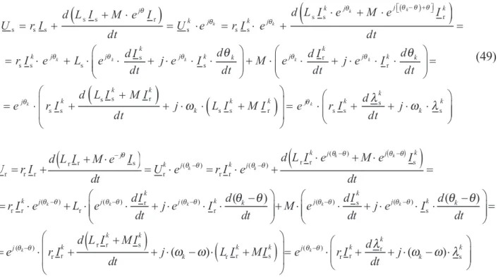
s r s s r s s s s s s s s r s s r s s s r s s s s k k k k k k k k k k j k j k j k j k j k k k j j j k k j j k k k k k j k d L I e M e I d L I M e I U r I U e r I e dt dt d d d I d I r I e L e j e I M e j e I dt dt dt dt d L I M I e r I j L dt θ θ θ θ θ θ θ θ θ θ θ θ θ θ θ ω − + ⋅ + ⋅ + ⋅ = + = ⋅ = ⋅ + = = ⋅ + ⋅ ⋅ + ⋅ ⋅ ⋅ + ⋅ ⋅ + ⋅ ⋅ ⋅ = + = ⋅ + + ⋅ ⋅(
)
s s r s s s k k k k j k k k d I M I e r I j dt θ λ ω λ + = ⋅ + + ⋅ ⋅ (49)(
)
(
( ) ( ))
r s r r s r ( ) ( ) r r r r r r ( ) ( ) r ( ) ( ) s ( ) r r s r r ( ) ( ) k k k k k k k k k k j j k j k j k j k k k j j j k k j j k k d L I e M e I d L I M e I U r I U e r I e dt dt d dI d dI r I e L e j e I M e j e I dt dt dt dt θ θ θ θ θ θ θ θ θ θ θ θ θ θ θ θ θ θ θ θ θ θ θ − − − − − − − − − − ⋅ + ⋅ + ⋅ = + = ⋅ = ⋅ + = − − = ⋅ + ⋅ ⋅ + ⋅ ⋅ ⋅ + ⋅ ⋅ + ⋅ ⋅ ⋅ (
r r s)
(
)
( ) ( ) r r r s r r ( ) r r ( ) s k k k k k k k k k k j j k k d L I M I d e r I j L I MI e r I j dt dt θ θ θ θ λ ω ω ω ω λ − − = + = ⋅ + + ⋅ − ⋅ + = ⋅ + + ⋅ − ⋅ (50) where ωk,ω are the angular velocity of the arbitrary reference frame, respectively the angular velocity of the induction machine. Finally, if we consider P the number of poles for the induction machine, the electrical angular velocity of the rotor is (P/2)ω and the vectorial equations of theinduction machine written in a common arbitrary reference frame which rotates with angular velocity ωk are: s s s s s r r r r r s r s s r s r r ( ) k k k k k k k k k k k k k k k k d U r I j dt d U r I j dt L I M I L I M I λ ω λ λ ω ω λ λ λ = + + ⋅ ⋅ = + + ⋅ − ⋅ = + = + (51-54)
The above equations system represent the mathematical model of the induction machine with stator and rotor equipped with one fictive windings each in a common arbitrary reference frame. It has to be highlighted that the mutual inductance does not depend on the relative rotor position (Kovacs -1984). Us Is U I r r θ k k k k k S R ω θ λ λ s k r k k k ω
Fig. 2.4.Model of the three-phase induction machine with fictive one stator winding and one rotor winding
(space vector notations) represented in a common arbitrary reference frame
2.5. Induction machine equations with stator referred rotor variables
A complete unified equations system for the induction machine is obtained when both stator and rotor variables are expressed in a common reference frame and the rotor variables are also stator referred. Using the turns ratio and the winding factor ratio we obtain:
r r t r t r r t r 2 r t r 1 ' ' ' ' I I k U k U k r k r λ λ = ⋅ = ⋅ = ⋅ = ⋅ (55-58)
Now the stator and rotor flux linkage equations can be written as:
(
)
s r s s
s mas s mas s mas t r
t 3 3 1 ' 2 2 k k k k k k L I L I L I k M I I k λ = ⋅ +σ ⋅ + ⋅ ⋅ =σ ⋅ ⋅ + ⋅ ⋅ + (59)
(
)
2 r s s rr mar r mar r mar t r t
t t 3 3 1 1 ' ' 2 2 k k k k k k L I L I L k I k M I I k k λ = ⋅ +σ ⋅ + ⋅ ⋅ = ⋅σ ⋅ ⋅ ⋅ + ⋅ ⋅ + (60)
If the following notations are introduced: ls s mas
L =σ ⋅L the stator leakage inductance 2
lr t r mar '
L =k ⋅σ ⋅L the rotor leakage inductance 2
M t mas t mar
3 3
2 2
L =k ⋅M= ⋅L = ⋅k ⋅L the main magnetisation inductance M s r
k k k
I = I +I the magnetisation current space vector M
M M
k k
L I
λ = ⋅ the magnetisation flux s
ls ls
k k
L I
λ = ⋅ the stator leakage flux lr lr r
'k L' I'k
λ = ⋅ the rotor leakage flux
The flux linkage equations get the following form:
s M s ls M ls M k k k k k L I L I λ = ⋅ + ⋅ =λ +λ (61)
(
M)
(
)
r lr r M lr M t t 1 1 'k L' I'k L Ik 'k k k k λ = ⋅ ⋅ + ⋅ = ⋅ λ +λ (62) or in referred variables we obtain:s s s ( ls M) M 'r s M 'r k k k k k L L I L I L I L I λ = + ⋅ + ⋅ = ⋅ + ⋅ (63) s s r lr M r M r r M 'k ( ' ) 'k k ' 'k k L L I L I L I L I λ = + ⋅ + ⋅ = ⋅ + ⋅ (64) whereLs and L’r are the total stator, respectively rotor self-inductance.
The referred rotor voltage is given now by the relation:
(
lr M)
(
)
r r r lr M ' ' ' ' ' 2 k k k k k k k d P U r I j dt λ λ ω ω λ λ + = + + ⋅ − ⋅ + (65)Finally we can write a complete equations system, in a common arbitrary reference frame, with rotor variables referred to the stator, which define the induction machine. The result is a mathematical model of the three-phase induction machine equipped with two fictive windings, rotating with angular velocity ωk. The simplified representation of this system is given in Fig. 2.5.
s s s s s r r r r r s s s M r s r r r M ' ' ' ' ( ) ' 2 ' ' ' ' k k k k k k k k k k k k k k k k d U r I j dt d P U r I j dt L I L I L I L I λ ω λ λ ω ω λ λ λ = + + ⋅ ⋅ = + + ⋅ − ⋅ = + = + (66-69) Us I s U I r r θ k k k k k S R ω θ λ λ s k r k k k ω
Fig. 2.5. Model of the three-phase induction machine with fictive one stator winding and one rotor winding (space vector notations) represented in a common arbitrary reference frame,
and referred rotor variables
2.6. Instanteous electromagnetic torque
The input power for a three-phase induction machine with wounded rotor is:
{
*}
{
*}
s r i s r 1 1 ( ) Re Re ' ' 2 2 k k k k P t = ⋅ ⋅m U ⋅I + ⋅ ⋅m U ⋅I (70) wherem is the phase number (3), U Usk, 'rk are the stator and rotor voltage space vectors, Isk*, 'I rk* are the conjugate stator and rotor current space vectors.Using a detailed relation for the space vectors with rotor variables referred to the stator, we get: i( ) as as bs bs cs cs 'ar 'ar 'br 'br 'cr 'cr
P t =U I +U I +U I +U I +U I +U I (71) From the complete equations system of the induction machine, the following expressions can be obtained for the input power of the machine:
* s * * * r * * s s s s i s s r r r r r r ' 3 Re ' ' ' ' ' ' 2 2 k k k k k k k k k k k k k k d d P P r I I I j I r I I I j I dt dt λ λ ω λ ω ω λ = + + ⋅ + + + ⋅ − (72) * * * * 2 2 s r s s i s s r r r s r r ' 3 Re ' ' ' ' ' 2 2 k k k k k k k k k k d d P P r I r I I I j I I dt dt λ λ ω λ ω ω λ = + + + + ⋅ + − (73) The first two terms from the power equation represent the Joule effect loss, the following two terms represent the electromagnetic power due to the time variation of the magnetic energy, and the last term stands for the mechanical power available at the machine shaft, if the hysterezis loss, eddy current loss and the stray losses are neglected. The mechanical power will be: