CFD modelling of transient pathogen release in indoor environments due to human activity

promoting access to White Rose research papers

White Rose Research Online

Universities of Leeds, Sheffield and York

http://eprints.whiterose.ac.uk/

White Rose Research Online URL for this paper:

http://eprints.whiterose.ac.uk/7699/

Published conference paper

Hathway, E.A., Sleigh, P.A. and Noakes, C.J. (2007)

CFD Modelling of Transient

Pathogen Release in Indoor Environments due to Human Activity.

In:

Proceedings of the 10th International Conference on Air Distribution in Rooms -

Roomvent 2007. Roomvent 2007, 13-15 June 2007, Helsinki.

CFD Modelling of Transient Pathogen Release in Indoor Environments due

to Human Activity

E.A.Hathway, P.A.Sleigh, C.J.Noakes

Pathogen Control Engineering Research Group, School of Civil Engineering, University of Leeds, LS2 9JT, UK

Corresponding email: [email protected]

SUMMARY

Certain routine hospital activities have been identified as a potential source for the airborne dispersal of micro-organisms. With increasing use of CFD to model hospital situations a method of modelling this type of spread within a simple steady state model is required. Since this type of dispersal will vary with space and time a single point source would not provide adequate information to represent these sources. Instead a zonal bioaerosol source is

introduced to represent the time average of the varying release from the activity. In this paper, data from experiments conducted in a bioaerosol test chamber are compared to CFD results. Numerical validation is also carried out comparing the zonal source to an equivalent transient source. The results indicate that the zonal source provides excellent comparison to the time averaged behaviour of a moving source, but greatly underestimates the maximum value at any one location.

INTRODUCTION

The dissemination of micro-organisms within indoor environments increases the potential for the rapid spread of disease. Many hospital patients are in some sense immuno-compromised and it is common that they are alongside patients who are suffering from infectious diseases. This close confinement provides a situation well suited to the dissemination and acquisition of infection[1].

There are several routes for the transfer of infection within the hospital environment, the most significant being that via hand contact between health-care workers and patients. However, infection through an airborne mechanism (if only partially) is also important. There are several mechanisms for micro-organisms to become airborne: being expelled by coughing and sneezing; through vomiting, diarrhoea, and through the natural shedding of skin particles. Certain routine activities in hospital wards can also cause a number of large particles, e.g. skin particles, to be dispersed into the environment. These particles may carry with them viable bacteria potentially capable of spreading disease. For instance it is well recognised that activities such as walking, undressing/dressing and bedmaking all disperse large numbers of bacteria into the air [2-6]. Within a busy hospital ward a significant level of activity occurs that could result in the dispersion of bacteria. Indeed our own studies have found that particles are frequently dispersed into the air within a respiratory ward and that activity may be

Computational Fluid Dynamics is an increasingly popular tool for detailed modelling of the movement of air and this basic technique can be extended to analyse the spread of

contaminants transported by an air flow. However most attempts at simulating a hospital ward do not account for many of the transient influences, preferring to consider a ‘freeze frame’, representative situation. A number of published works using CFD to model bio-aerosol spread in hospitals have considered respiratory infections such as SARS [9-11]and Tuberculosis [12]. In all of these cases a directed point source is used to represent the dispersal of particles from a cough, which is appropriate where the patient is primarily bed bound. Some interesting recent work by Brohus et al [13] highlighted the need for considering the effect of movement

on airflow patterns in an operating room situation. They found that movement could cause the transport of bioaerosols from the non-clean area of the operating room to the clean area and used a simple model that included distributed momentum sources and a turbulent kinetic energy source to simulate the influence of movement on the air flow. However, despite the obvious potential for pathogens to be released through general ward activity, the use of CFD to directly model the spread of particles in this manner has not been considered. As CFD is increasingly being used to model hospital situations, a method of easily modelling this airborne dispersal of infectious material may lead to a greater understanding of the spread of disease within the ward environment.

This study considers how to represent the dispersion of micro-organisms that are shed from the human skin during activity. Activity related dispersal may occur over a large area varying in position and rate with time as people move about the hospital, carrying out different tasks. A detailed transient model of this situation would not only use an unfeasible amount of CPU, but would provide misleadingly detailed information about a situation that would change continuously. This study aims to develop a representative method for modelling the

dispersion from a bacteria source that varies in time and space, within a steady state model. The study introduces the concept of using a ‘zonal’ source that time averages the dispersion over the area in which the activity occurs. In order to assess the validity of this zonal representation, experiments are carried out in a bioaerosol test chamber under controlled environmental conditions, introducing bacteria across a zone. The dispersion pattern from this is compared to a CFD model using a zonal source. Numerical validation is then carried out using this model to assess the suitability of using a zonal source instead of a point source to represent the dispersion of bacteria from a transient source. Steady state models are developed to model the dispersion from the point and zonal source and the dispersion patterns from these are compared to a transient model of a bioaerosol point source that moves through the space.

METHODS

Experimental Methods

All experiments were carried out in a climatically controlled aerobiological test chamber at The University of Leeds. This is a hermetically sealed 32.25m3 (3.35 x 4.26 x 2.26m) room with a controlled, hepa filtered ventilation system. Air is supplied to the room through an inlet at low level and extracted near the ceiling as shown in figure 1 (Inlet A/Outlet A).

Bioaerosol Source

A pure culture of Serratia marcescens suspended in distilled water was aerosolised using a six

set of holes is rotated by 45°.This is centred at a height of 1.15m and bioaerosols are emitted starting 0.42m from the wall over a space of 1.2m. As shown in figure 2. Serratia

marcescens was used to create the

bio-aerosols. This particular bacterium was chosen as it is easy to grow on nutrient agar, poses minimal risk and the colonies are pink, enabling any contamination from other sources to stand out.

During the experiments the ventilation rate was set at a constant rate and the nebuliser operated continuously to maintain a steady-state bioaerosol concentration in the chamber. Before any samples were taken the air flow and the nebuliser were allowed to run for 45 minutes to achieve this steady-state. Air samples were then taken from the test chamber through 5mm tubes pulling air out at 12 points spaced equally in the room as shown in figure 2. The sampling

locations were at the same height as the bioaerosol inlet, 1.15m above floor level. An Anderson sampler was used to take the air samples, impacting the bacteria onto nutrient agar. Only levels 5 and 6 of the Anderson sampler were used, relating to bioaerosol sizes of smaller than 2μm. Samples were taken from each of the 12 points in the room, every 10 minutes, with 44 litres of air sampled in each case. This was then repeated 8 times with the order of sampling varied. After incubating overnight

at 37oC the microbial colonies on the plates were counted and positive hole correction applied

[14] to quantify the concentration in terms of colony forming units per cubic metre (cfu/m3_).

Description of CFD Model

Airflow Simulation

The CFD analysis of the test chamber was carried out using Fluent 6.1.22. Two 3D models were created of a 32.25m2 (3.35 x 4.26 x 2.26 high) room with geometry as shown in figure 1 to simulate two different ventilation regimes. A tetrahedral grid was used containing approx 540,000 cells with refinement around the inlet, outlet and bacterial source. A grid refinement study was carried out prior to choosing this mesh. A standard k-ε turbulence model was used with enhanced wall treatment and a no slip condition was applied at the walls. The model was treated as isothermal as there were no heat sources within the test chamber during the

experiments and the incoming air temperature was controlled.

Velocity inlets were defined to simulate an air change rate of 6 AC/h for the two different ventilation regimes. Ventilation regime A used a low to high ventilation system as shown by Inlet A/Outlet A in figure 1. The angled louvers on the inlet were represented by describing

Figure 1: Schematic of the Room geometry

Figure 2: Plan of room showing bioaerosol source for experimental validation and sampling points.

z

x 0.67m

0.67m 0.63m 0.63m 1m 1m 1m

1m

1m

Bioaerosol Source Sample Point CFD Sampling Line

i l

the inlet velocity as a series of velocity profiles resulting in an average velocity of 0.04m.s-1, 10mm in front of the inlet. The extract was modelled as a zero pressure boundary (with 0 Pa imposed).

In order to consider the effect of the zonal source with a different air flow pattern in the numerical validation, a second method, regime B, using ceiling mounted diffusers was defined. This is shown in figure 1 by Inlet B/Outlet B. Air enters the space with a speed of 0.59m.s-1, at a downwards angle of 45°, from vertical slits 60mm deep. The extract was treated again as a zero pressure boundary.

Bioaerosol Distribution

For this study the bioaerosols were assumed to remain airborne for long periods of time which is suitable for small micro-organisms 2μm in diameter or less. With this assumption it is reasonable to use a passive scalar to model the bacterial sources. The movement of the bacteria within the space was therefore solved using the scalar transport equation:

( )

(

)

∂

∂φ _{φ φ}

grad div div

t u , (1)

Where φ is the concentration of micro-organisms per unit volume (quantity.m-3); u is the velocity vector (u,v,w) of the air (m.s-1); and Γ is the diffusivity (m2.s-1).

Natural decay of viable micro-organisms in the space is not considered in this case. The diffusivity of the bio-aerosols is set to 1x10-7m2.s-1.

CFD Source definition for Experimental Validation

A zonal source was set up to represent the injection of bacteria over an entire zone 0.1 x 0.1 x 1.2 m long, located as shown in figure 2. A small volumetric momentum source was applied to represent the expulsion into the air that these particles will receive, for which 0.1 N.m-3 was added in all directions around the edge of the source. Sensitivity tests were carried out on adding this volumetric momentum source, and since it is over a thin area it does not affect the global room air flow.

CFD Source definition for Numerical Validation

In order to validate the zonal source model, dispersion from this and a point source were compared to an equivalent transient source moving through the space. These three different types of bioaerosol source are described below.

Transient Source: The scalar source is applied over a small cube 0.1m3 this moves through

the space at 1.2x10-3 _m.s-1_{. For case 1 (figure 1a) this moves in the z direction through 3m}

across the centre of the room, with the initial position at z = 0.42m. For case 2 the source moves in the x direction starting at x = 0.33m, for 3.93m. A slow speed was chosen in order to ensure there was large amount of dispersion during the time the source is moving. A momentum source was added as detailed above. This model is used to find the time averaged scalar values across the space, the volume average scalar values and the maximum value in the space over the whole time.

Zonal Source: The zonal source was set up to inject the same overall scalar quantity into the

long and runs across the centre of the room in the z direction. For case 2 the zonal source is 0.1 x 0.1 x 3.6m running in the x direction centrally in the room. A momentum source is added at the edge of the whole zone as before.

Point Source: The point source is positioned in the centre of the room; and therefore the

centre of the zonal source. The same quantity of scalar is again dispersed into the space over a volume of 0.1m3 with a small volumetric momentum source of 0.1N.m-3 defined at the edges.

Solution Process

Second order discretisation of the governing equations was used over the whole domain and solutions found using a segregated, implicit solver. The solution was considered to be converged when the residuals were less than 5 x 10 -4 and the net imbalance of mass flow within the space was less than 0.1%.

The air flow was considered as steady state for all cases however the scalar transport equation was solved transiently to simulate the moving source. A first order implicit solution was carried out using a time step of 10s. This was chosen by running a series of models with times steps of 1s, 10s, 100s. The results with a time step of 10s were deemed to be of a suitable accuracy when compared to a 1s time step, hence this was chosen for the final model.

RESULTS

Experimental Validation of Zonal Source

The experimental results showed a large amount of variation for each point. This variation is to be expected as turbulence factors in the room will affect the

movement of the contaminant. The process of spraying micro-organisms into the room and sampling by impaction onto an agar plate is highly stressful and will lead to some organisms dying, which will also increase the variance of the results.

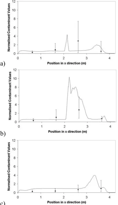
In order to compare the experimental and CFD results for a zonal source, the computed bioaerosol concentration was plotted along three lines running in the x direction at the height of the experimental sampling plane. These lines are shown in figure 2. The experimental sample point values were averaged and normalised around the total average for the plane during one experimental run. These values were plotted on the same figures (figure 3), together with error bars to show the

variance in the experiments. Figure 3 shows the general trend in the experiment is reflected in the CFD model. There are

a)

b)

c)

some differences in the results, particularly close to the source; this is likely to be due sampling a volume in the experiment but taking point values from the CFD results. All the points fall within the experimental error bars, indicating the maximum and minimum values sampled, or very close to them. Figures 4a and b show concentration contours on the horizontal sampling plane. The pull towards the inlet side of the source is visible in both the experimental and CFD results. Figure 4c shows clearly where there are higher build ups of bio-aerosols in 3 dimensions.

a) b) _c)

Figure 4: Contours of bioaerosol values on plane y = 1.15m a) experimental results, b) CFD results. c) Plume showing 3D dispersal pattern from the zonal source in CFD.

Numerical Validation of Zonal Source

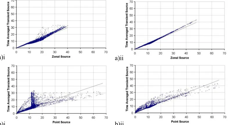
To numerically compare the dispersion patterns from the three sources; transient, zonal and point, plots of scalar concentration values were produced on x-z planes, y = 1.15m, the height of the source, and y = 1.60m, representing the breathing height of a standing person. The scalar values at each cell were output in each case. In order to assess the ability of the zonal source in representing the time averaged behaviour of a transient source, scatter plots of the two results were created to show the correlation between them. This was also carried out to compare the transient source to the point source

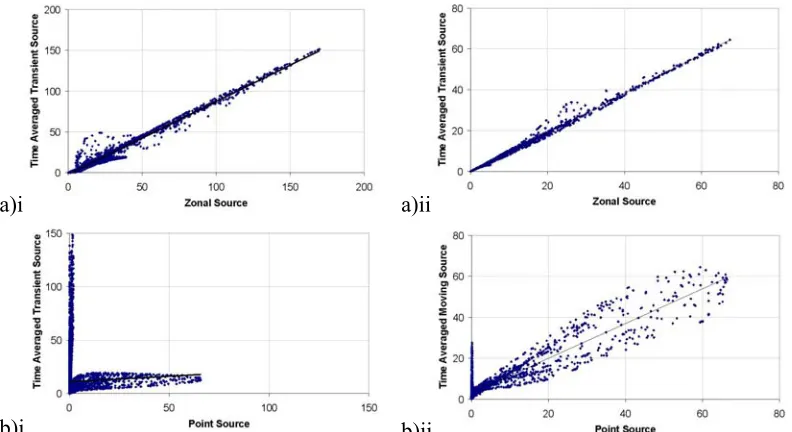
For the two different ventilation regimes, orientation of sources and planes of results the graphs show clearly that the time averaged dispersion from the transient source is more closely represented by a zonal source than a central point source (figures 5-8). Statistical analysis showed that the correlation of the zonal source is consistently close to the time averaged with values of r2 over 0.84 (table 1). When using the point source the correlation to the time averaged model improves as the sample plane is moved further from the source. For instance figure 6bii shows very good correlation using a point source. But this is not always the case, figure 8bi shows very poor correlation with the point source even on the plane at y = 1.60m. Depending on the position of the source and the ventilation regime the correlation for a point source varies greatly.

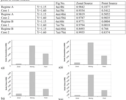
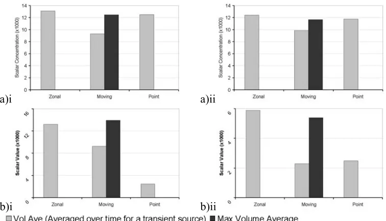
However, the zonal source greatly underestimates the maximum scalar value in the room. For ventilation regime A, case 1, the maximum value for the point source is much closer to the transient source than the zonal source (figure 9a). However comparing the maximum values in the room with the other regimes show even the results from the point source model give very low maximum values in the room relative to the transient source. In these cases the zonal model gives a maximum scalar value that is only 4-9% of the value for the transient source. This may be because, depending the source position, the scalar will get caught in areas of recirculation which leads to a large build up over time. The zonal source tends to over

estimate the time average of the volume average in the space (figure 10) but is representative of the maximum volume average that occurs throughout the whole time period.

a)i _a)ii

b)i b)ii

Figure 5: Scalar concentration (x1000) at each cell. Ventilation Regime A. Sample plane y=1.15m. a) zonal source against the time averaged values from a transient source b) Point source against the time averaged values from a transient source i) Case 1 ii) Case 2.

a)i a)ii

b)i b)ii

a)i a)ii

b)i _b)ii

Figure 7: Scalar concentration (x1000) at each cell. Ventilation Regime B. Sample plane y=1.15m. a) zonal source against the time averaged values from a transient source. b) Point source against the time averaged values from a transient source. i) Case 1 ii) Case 2.

a)i a)ii

b)i b)ii

Figure 8: Scalar concentration (x1000) at each cell. Ventilation Regime B. Sample plane y=1.60m. a) zonal source against the time averaged values from a transient source b) Point source against the time averaged values from a transient source i) Case 1 ii) Case 2.

DISCUSSION

source; whereas the ability of a point source to do the same is generally poor and varies greatly on the position of the source and the ventilation regime. In order to predict the average dispersal pattern of bioaerosols in hospital wards from activities the use of a zonal source will therefore be more suited. The zonal source may be applicable for modelling situations such as bedmaking, or general nursing activities around a bed, where the bacteria will be dispersed over the entire zone of the bed.

Although this method gives a reasonable representation of the position of the maximum value of contamination in the space it will greatly underestimate the magnitude of this maximum. In order to find this maximum value it is necessary that the dispersion pattern is known, a point source will only give a reasonably acceptable value if it is positioned in the correct place. It

may be possible to scale up the value acquired from the zonal source but further work is needed in order to assess the value for this scaling.

Since the concept of the zonal source is to represent the activity from people further work will be carried out including a source of heat with the scalar. The skin particles the zonal source is intending to represent may be larger than 5μm, and so future work will be carried out using a lagrangian approach, including the effect of the size and mass of the particles.

Table 1: r2 values showing the correlation between the time average moving source and a point or zonal source.

Fig No. Zonal Source Point Source

Y=1.15 4ai/4bi 0.9842 0.1877

Regime A

Case 1 Y=1.60 5ai/5bi 0.9554 0.5412

Y=1.15 4aii/4bii 0.9819 0.5052

Regime A

Case 2 Y=1.60 5aii/5bii 0.9787 0.9035

Y=1.15 6ai/6bi 0.9771 0.0004

Regime B

Case 1 Y=1.60 7ai/7bi 0.9794 0.0018

Y=1.15 6aii/6bii 0.8493 0.766

Regime B

Case 2 Y=1.60 7aii/7bii 0.9955 0.8374

a)i a)ii

b)i _b)ii

a)i a)ii

b)i b)ii

Figure 10: Volume Averaged Scalar values within the room. a)Ventilation Regime A. b)Ventilation Regime B i) Case 1 ii) Case 2.

REFERENCES

1. Parker, M T. Transmission in Hospitals. in International Symposium on Aerobiology (4th).

1972. Technical University at Enschede, The Netherlands: Utrecht Oosthoeck.

2. Speers, R, Bernard, H, Ogrady, F, and Shooter, R A, Increased Dispersal of Skin Bacteria into

Air after Shower-Baths. Lancet, 1965. 1(7383): p. 478-480.

3. Noble, W C, Dispersal of Skin Microorganisms. British Journal of Dermatology, 1975. 93(4):

p. 477-485.

4. Duguid, J P and Wallace, A T, Air Infection with Dust Liberated from Clothing. Lancet, 1948.

255(NOV27): p. 845-849.

5. May, K R and Pomeroy, N R. Bacterial dispersion from the body surface. in Airborne

Transmission and Airborne Infection: 4th International Symposium on Aerobiology. 1973.

Technical University at Enschede, The Netherlands: Oosthoek Publishing Company.

6. Hare, R and Thomas, C G A, The Transmission of Staphylococcus Aureus. British Medical

Journal, 1956. 2(OCT13): p. 840-844.

7. Roberts, K, Hathway, A, Fletcher, L A, et al., Bioaerosol production on a respiratory ward.

Indoor and Built Environment, 2006. 15(1): p. 35-40.

8. Thornton, T, Fletcher, L A, Beggs, C B, et al. Airborne Microflora in a Respiratory Ward. in

American Society of Heating, Refrigeration and Air Conditioning Engineer. Indoor Air

Quality Conference. 2004. Tampa, Florida.

9. Wong, T W, Lee, C K, Tam, W, et al., Cluster of SARS among medical students exposed to

single patient, Hong Kong. Emerging Infectious Diseases, 2004. 10(2): p. 269-276.

10. Li, Y, Huang, X, Yu, I T S, et al., Role of air distribution in SARS transmission during the

largest nosocomial outbreak in Hong Kong. Indoor Air, 2005. 15(2): p. 83-95.

11. Chau, O K Y, Liu, C H, and Leung, M K H, CFD analysis of the performance of a local

exhaust ventilation system in a hospital ward. Indoor and Built Environment, 2006. 15(3): p. 257-271.

12. Noakes, C J, Sleigh, P A, Escombe, A R, and Beggs, C B, Use of CFD analysis in modifying a

TB ward in Lima, Peru. Indoor and Built Environment, 2006. 15(1): p. 41-47.

13. Brohus, H, Balling, K D, and Jeppesen, D, Influence of movements on contaminant transport

in operating room. Indoor Air, 2006. 16(5): p. 356-372.

14. Macher, J M, Positive-Hole Correction of Multiple-Jet Impactors for Collecting Viable