This is a repository copy of
Solar feature tracking in both spatial and temporal domains
.
White Rose Research Online URL for this paper:
http://eprints.whiterose.ac.uk/10582/
Proceedings Paper:
Jess, D.B., Mathioudakis, M., Erdelyi, R. et al. (3 more authors) (2007) Solar feature
tracking in both spatial and temporal domains. In: Erdelyi, R. and Mendoza-Briceno, C.A.,
(eds.) Waves & Oscillations in the Solar Atmosphere: Heating and Magneto-Seismology.
IAU Symposium 247, September 17-22, 2007, Porlamar, Isla de Margarita. Proceedings of
the International Astronomical Union, 3 (s247). Cambridge University Press , Cambridge ,
pp. 288-295. ISBN 978-0-52187-4694
https://doi.org/10.1017/S1743921308014981
[email protected] https://eprints.whiterose.ac.uk/
Reuse
Unless indicated otherwise, fulltext items are protected by copyright with all rights reserved. The copyright exception in section 29 of the Copyright, Designs and Patents Act 1988 allows the making of a single copy solely for the purpose of non-commercial research or private study within the limits of fair dealing. The publisher or other rights-holder may allow further reproduction and re-use of this version - refer to the White Rose Research Online record for this item. Where records identify the publisher as the copyright holder, users can verify any specific terms of use on the publisher’s website.
Takedown
If you consider content in White Rose Research Online to be in breach of UK law, please notify us by
Heating and Magneto-Seismology
Proceedings IAU Symposium No. 247, 2007 R. Erd´elyi & C. A. Mendoza-Bricen˜o, eds.
c
2008 International Astronomical Union doi:10.1017/S1743921308014981
Solar feature tracking in both spatial and
temporal domains
D. B. Jess
1,2, M. Mathioudakis
1, R. Erd´
elyi
3, G. Verth
3, R. T. J.
McAteer
2and F. P. Keenan
11Astrophysics Research Centre, School of Mathematics and Physics, Queen’s University, Belfast, BT7 1NN, Northern Ireland, UK
email:[email protected]
2NASA Goddard Space Flight Center, Solar Physics Laboratory, Code 671, Greenbelt, MD 20771, USA
3SP2RC, Department of Applied Mathematics, The University of Sheffield, Sheffield, S3 7RH, England, U.K.
Abstract. A new method for automated coronal loop tracking, in both spatial and temporal domains, is presented. The reliability of this technique was tested with TRACE 171˚A obser-vations. The application of this technique to a flare-induced kink-mode oscillation, revealed a 3500 km spatial periodicity which occur along the loop edge. We establish a reduction in oscilla-tory power, for these spatial periodicities, of 45% over a 322 s interval. We relate the reduction in oscillatory power to the physical damping of these loop-top oscillations.
Keywords. Sun: activity, Sun: atmospheric motions, Sun: corona, Sun: evolution, Sun: flares, Sun: oscillations
1. Introduction
Automated feature recognition and tracking has long been a goal for scientists. With the advent of higher sensitivity satellite-based telescopes and the resulting increase in readout rates, it is imperative to be able to analyse, at least to some minimal level, data “on the fly”. Without this ability, the large data rates achievable make it extremely dif-ficult to implement onboard trigger programmes (e.g. a flare trigger), which allow the telescope pointing to be redirected to an area of interest and modify the instrument observing mode, almost immediately. Furthermore, having a means of establishing in-teresting phenomena occurring on the Sun in real time allows instrument users to pick datasets of interest much more readily than in the past. Thus, many schemes have been setup to push this form of real-time data analysis forward, including the Heliophysics Knowledge Base programme, which will enable real-time detections of oscillatory phe-nomena occurring on the Sun.
Current orbiting solar satellites, in particular theTransition Region And Coronal Ex-plorer,trace, have enabled the analysis of many oscillatory signatures originating within
the outer atmosphere of the Sun. Wang & Solanki (2004), Marsh & Walsh (2006) and Schrijver et al. (2002) all report oscillatory phenomena occuring within coronal loop structures, thus demonstrating the need for automated, oscillation detection software. Previously, however, the majority of work on oscillating coronal loops has been focussed on the temporal domain (see latest review in Banerjee et al. 2007). In this work, we investigate the spatial evolution of a coronal loop structure, a method proposed first by Erd´elyi & Verth (2007); Verth et al. (2007), independent of its position during a flare-induced kink oscillation. From this we can understand the behaviour of the loop, in the
Solar feature tracking in both spatial and temporal domains 289
spatial domain, and establish any phenomena which are flare induced, yet confined to the volume occupied by the loop. In§2 we describe the observations under investigation, while in§3 we discuss the methodologies used during the analysis of the data which allow us to accurately track the spatial evolution of coronal loops. A discussion of our results in the context of confined loop oscillations is given in § 4, and finally, our concluding remarks are given in §5.
2. Observations
The data presented here are part of an observing sequence obtained on 1998 July 14, using the traceimaging satellite. The optical setup of trace allowed a 384′′ ×384′′
region surrounding active region NOAA 8270 to be investigated with a spatial resolution of 1′′(0.5′′per pixel). The filter selected for these observations was the 171˚A filter, which
has an inherent passband width of 6.4˚A, allowing plasma in the temperature range 0.2–
2.0 MK to be studied. The cadence of the trace instrument was not constant during
the observing sequence, with the time between successive exposures varying between 66 and 82 s. The observations employed in the present analysis consist of 88 successive
traceimages providing nearly two hours of continuous, uninterrupted data. During the
observing sequence, a large M4.6 flare occurred in the immediate vicinity of the active region under investigation.
3. Data Analysis
3.1. Initial Image Processing
Thetracedata was retrieved directly from the Lockheed Martin Solar and Astrophysics
Labs database and was subjected to common processing algorithms. The idl routine
trace prep.pro was implemented calling appropriate keywords to remove cosmic-ray
streaks, reduce readout noise and prepare the data in a user-friendly format. De-rotation of the traceimages was also deemed necessary, since the observing sequence lasts
ap-proximately two hours, equating to a relatively large solar rotation (20′′at disk centre).
From this point, it was possible to use additional programmes to aid in the analysis of the data as described in detail below.
3.2. Laplacian Image Sharpening
The Laplacian operator is a second order method of enhancement and is particularly good at finding fine detail in an image. Any feature with a sharp discontinuity (such as noise) will unfortunately be enhanced by a Laplacian operator, however this method of image enhancement is often used when spatial resolutions are less than desirable. Thus, one application of the Laplacian operator is to restore fine detail to an image which has been smoothed, or pre-processed, to remove noise (eg using a median filter). The Laplacian operator is implemented as a convolution between an image and a kernel. The kernel can be constructed in various ways, but we use the 3-by-3 kernel implemented by Gonzalez & Woods (1992).
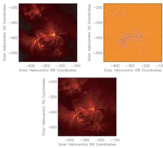
In image convolution, the kernel is centered on each spatial pixel in turn, and the pixel value is replaced by the sum of the kernel mutipled by the image values. With the particular kernel implemented here, we are counting the contributions of the diagonal pixels as well as the orthogonal pixels in the filter operation. This is not always necessary or desirable, although it works well here, as will be demonstrated. Figure 1 shows the result of appling the convolution kernel to thetraceimage, as well as the final output
Figure 1. Complete trace field of view (top left) after undergoing initial processing using
thetrace prep.pro idlroutine. The top right image shows the fine-scale structures detected
using the Laplacian filter outlined in§3.2 and the bottom image reveals the sharpenedtrace
field of view after the addition of fine-scale structures. Note how the clarity of loop structures is drastically increased.
the emphasis of fine structures when compared to the original, unfiltered image. For the purposes of the data under investigation here, all traceimages were subjected to
Laplacian image sharpening routines.
3.3. Wavelet Modulous Maxima Edge Detection
After sucessful completion of image sharpening, edge detection algorithms can be imple-mented. The sharpened images have increased fine-scale information and as such provide the necessary platform for establishing feature edges which may have been previously unresolvable. Immediately after the flare event, one particular coronal loop is seen to oscillate. This kink-mode oscillating loop has been investigated previously (see Aschwan-den et al. 1999 for the initial investigation) in the temporal domain. Here, we will in-vestigate the behaviour of the loop in the spatial domain. In order to track the spatial behaviour of the loop, a fully automated routine was devised to minimise errors intro-duced through human interaction with the data.
The first step involves intensity thresholding whereby features in the trace
Solar feature tracking in both spatial and temporal domains 291
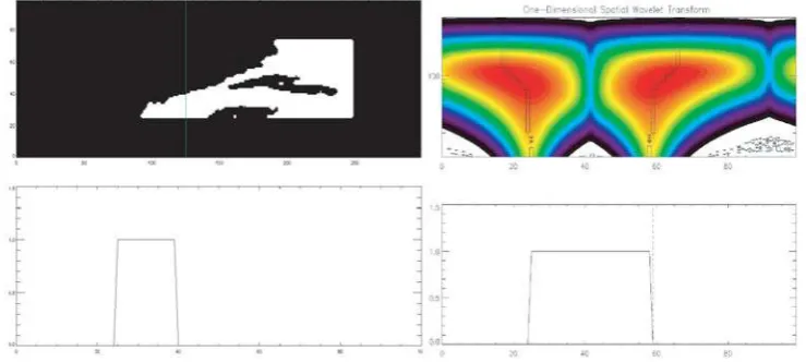
Figure 2.Upper-left panel shows the binary-formatted image obtained through intensity thresh-olding inserted into a padded, zeroed array which provides the best platform for WMM edge detection. The axis scales are pixel number with 1 pixel = 0.5′′. The vertical green line cor-responds to x pixel element 125 with the resulting intensity plot for this x pixel shown in the bottom-left panel. The corresponding wavelet power spectrum (top right) generated along the vertical spatial direction of thetracefield of view for horizontal pixel number 125. This panel
also shows regions of maximum power being traced down to the intersect point on the x-axis. The intensity plot (same as lower left) is again plotted (bottom right) with a dashed line indicating the position of intersection of the maximum wavelet power traces with the x-axis. Notice how the x-axis intersect position of maximum wavelet power corresponds exactly to the reduction of intensity in the bottom panel. This reduction in intensity is analagous with the upper edge of
thetracecoronal loop showing the accuracy of this method when detecting feature edges.
To emphasize feature edges and remove shallow intensity gradients, a binary format for feature mapping is used. All pixels which lay above the lower intensity threshold defined above are assigned a value of ‘1’. Those pixels which lay below the threshold were assigned a value of ‘0’ as seen in Figure 2. This binary format provides an absolute intensity cut-off thus providing a definite feature edge which can be tracked, both spatially and temporally. The binary image is padded using a zeroed array from which feature edge tracking can commence.
Tracking of this feature edge is performed using a Wavelet Modulous Maxima (WMM) technique (Muzy et al. 1993, McAteer et al. 2007). From the padded binary array created above, a horizontal pixel is chosen. Figure 2 shows the selection of horizontal pixel 125, as indicated by the vertical green line, as well as the corresponding intensity plot along this vertical line. A wavelet transform is produced for this intensity plot, demonstrated in the right-hand panel of Figure 2, utilizing a Mexican Hat wavelet. A Mexican Hat wavelet is very useful for detecting sharp intensity gradients which are present due to the binary format implemented above. An absolute wavelet power spectrum is plotted as a function of vertical pixel element in Figure 2. Additionally, maximum wavelet power features are traced down to the x-axis of the power spectrum and reveal the locations of maximum intensity gradients. Figure 2 re-plots the intensity in the vertical direction at horizontal pixel 125 and it can be seen that where the maximum wavelet power meets the x-axis also corresponds to the edges of thetracecoronal loop under investigation.
such features closer to the centre of active regions. Since in this instance it is desirable to track the upper edge of the coronal loop, we disregard the first maximum wavelet power location and record the position where the second maximum wavelet power location intersects with the x-axis. This pin-points the exact location of the Northerly edge of the coronal loop in question. This process is repeated over the entire E/W direction, and for all frames in the observing sequence, with the subsequent position of the Northern edge of thetracecoronal loop recorded. From the resulting loop edge positions, it is possible
to analyse both temporal and spatial variations.
4. Results and Discussion
It is our main goal to investigate the spatial behaviour of the oscillating coronal loop, as mentioned in § 3.3. However, to verify that the presented loop-tracking routine is functioning properly, derived results in the temporal domain are compared to previous findings. Examining the temporal behaviour of the detected coronal-loop edge, a peri-odicity of approximately 300 s exists which is consistent with the findings of Aschwan-den et al. (1999). This result implies that the loop detection and tracking algorithms, developed here, are functioning accurately, as temporal variations of loop position are consistent with previously published results.
From examination of the trace time series, it appears that the oscillating coronal
loop passes through an equilibrium position at times of 0, 280 and 602 s, with the overall shape of the loop similar at the correspondingtraceframes. If indeed the shape of the
loop is identical at times of 0, 280 and 602 s, then a subtraction of any two of these loop shapes should provide a resulting image equal to zero. However, upon subtraction of the loop shape at 0 s from that at 280 s, a spatial periodicity is revealed. Running this resulting loop shape through a one-dimensional spatial wavelet transform establishes an oscillatory period along the Northern loop edge of 10 pixels (Fig. 3). A number of strict criteria implemented on the data allowed us to insure that oscillatory signatures correspond to real periodicities. These criteria have been described in detail in previous papers (see Banerjee et al. 2001, Jess et al. 2007, McAteer et al. 2004). With thetrace
plate scale equal to 0.5′′ per pixel, the detected 10 pixel periodicity corresponds to an
absolute spatial distance of approximately 3500 km per complete oscillation (more than three complete cycles detected).
To see if this periodicity is visible at the following equilibrium position (602 s), we subtract the loop shape at 0 s from that at 602 s, and pass through our one-dimensional spatial wavelet transform. The resulting evidence indicates that the 10 pixel spatial pe-riodicity is indeed still present, albeit with a reduction in oscillatory power. We interpret the reduction in oscillatory power as the physical signature of damping of the loop-top oscillations. A closer inspection reveals that the oscillatory power has dropped by 45% during the 322 s interval, remaining consistent with other aspects of coronal-loop oscil-lations, which are seen to be heavily damped (Aschwanden et al. 2003, Ruderman 2005, Terradas et al. 2006, Dymova & Ruderman 2007).
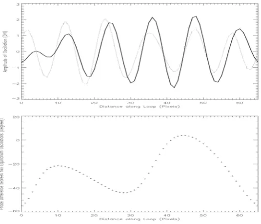
To investigate a possible phase relationship (Athay & White 1978), we create a cross-wavelet power spectrum between the two detected loop-top oscillations, and inspect the resulting spatial-phase diagram (Fig. 4). This figure reveals a clear phase shift, over many complete wavelengths, in the order of 0◦ to −50◦. Of course, due to the long
kink-oscillation period (≈300 s), and the relatively poor, and irregular, cadence of the
traceinstrument, we are only able to evaluate kink-equilibrium spatial periodicities at
Solar feature tracking in both spatial and temporal domains 293
Figure 3.Detection of a 10 pixel spatial oscillation. The resulting Northern loop-edge outline created by the subtraction of the loop edge at 0 s from the loop edge at 280 s after the flare event is shown in a). The one-dimensional spatial wavelet power transform along with locations where detected power is at, or above, the 99% confidence level are contained within the contours in b). Plot c) shows the summation of the wavelet power transform over time (full line) and the Fast Fourier power spectrum (crosses) over time, plotted as a function of period. Both methods have detected a well pronounced 10 pixel spatial oscillation. The global wavelet (dotted line) and Fourier (dashed dotted line) 95% significance levels are also plotted. The cone of influence (COI), cross-hatched area in the plot, defines an area in the wavelet diagram where edge effects become important and as such any frequencies outside the COI are disregarded. Periods above the horizontal line (dotted) fall within the COI. The probability levels, which are related to the percentage confidence attributed to the peak power at every time step in the wavelet transform, are plotted in d).
the loop prior to the flare-induced kink oscillation. Between these two equilibrium states, the loop in question has underwent one complete kink-oscillation cycle. If this loop-top oscillation is a propagating wave using the confines of the coronal loop as a waveguide, then it must exhibit a velocity matching the Alfv´en speed. Assuming an Alfv´en speed of
≈1000 km/s (Nakariakov & Verwichte 2005), and using the time interval (322 s) between successive equilibrium positions, we can derive a traversed distance for the loop-top wave equating to≈0.32 Mm (equivalent to 88.9 periods). Subtracting complete periods from this value (88.9 - 88), we are left with 0.9, which corresponds to a phase of 324◦. This is
comparable to the 0◦to −50◦ phase relation shown in Fig. 4.
Figure 4.The top panel shows the oscillation amplitude as a function of position along the loop for both loop-top oscillations. The solid line relates to the spatial periodicity detected between times of 0 and 280 s, while the dotted line relates to the spatial periodicity detected between times of 0 and 602 s. From this plot, it is clear to see a phase shift between the two loop-top oscillations. The bottom panel shows the phase-difference results of a cross-wavelet spectrum of the two detected spatial oscillations. We can clearly see a phase shift, on the order of 0◦ to
−50◦, over the duration of 6 complete cycles.
coronal loops away from the region under investigation, yet within the sametracefield
of view. Since these loops are not connected with the flare event, and therefore not seen to oscillate, no spatial periodicities along the loop would be expected when two loop outlines are subtracted from one and other. Subtracting the control loop outline at 0 s from that at 280 s after the flare, to remain consistent with the work above, and running through a one-dimensional spatial wavelet transform reveals no periodicities. Furthermore, we tested for spatial periodicities, on the loop seen to oscillate, both prior to, and long after, the flare event. These tests found no oscillatory phenomena in either instance, indicating that the spatial periodicities detected are flare induced.
5. Concluding Remarks
A new method for the detection, and subsequent tracking, of coronal loop structures is presented. This method also provides the ability to simultaneously search for longitudinal and transverse oscillations in real-time. This is particularly useful for future space-bourne solar telescopes, where the large achievable data rates will make real-time data analysis paramount. Utilizing our method for automated coronal loop analysis, we have detected spatial periodicities, on the order of 3500 km per cycle, occurring on a coronal loop immediately after being buffeted by a neighbouring M4.6 flare. We detect the damping of these loop-top oscillations, with a 45% reduction in oscillatory power over a 322 s interval. We also detect a wrapped spatial phase shift of 0◦ to −50◦, related to the
Solar feature tracking in both spatial and temporal domains 295
Acknowledgements
DBJ wishes to thank the Department for Employment and Learning and NASA’s Goddard Space Flight Center for a studentship. RE is grateful for an IAU travel grant, acknowledges M. K´eray for patient encouragement, and, is also grateful to NSF, Hungary (OTKA, Ref. No. K67746). Wavelet software was provided by C. Torrence and G. Compo.
References
Aschwanden, M. J., Fletcher, L., Schrijver, C. J., & Alexander, D., 1999,ApJ, 520, 880 Aschwanden, M. J., Nightingale, R. W., Andries, J., Goossens, M., & Van Doorsselaere, T.,
2003,ApJ, 598, 1375
Athay, R. G., & White, O. R., 1978,ApJ, 226, 1135
Banerjee, D., Erd´elyi, R., Oliver, R. & O’Shea, E., 2007,Sol. Phys, 246, 3 Banerjee, D., O’Shea, E., Doyle, J. G., & Goossens, M., 2001,A&A, 371, 1137 Dymova, M. V., & Ruderman, M. S., 2007,A&A, 463, 759
Erd´elyi, R. & Verth, G., 2007,A&A, 642, 743
Gonzalez, R., & Woods, R., 1992, Digital Image Processing, Addison Wesley, 414
Jess, D. B., Andi´c, A., Mathioudakis, M., Bloomfield, D. S., & Keenan, F. P., 2007,A&A, 473, 943
McAteer, R. T. J., Gallagher, P. T., Bloomfield, D.S., Williams, D. R., Mathioudakis, M., & Keenan, F.P., 2004,ApJ, 602, 436
McAteer, R. T. J., Young, C. A., Ireland, J., & Gallagher, P. T., 2007,ApJ, 662, 691 McEwan, M. P., & De Moortel, I., 2006,A&A, 448, 763
Marsh, M. S., & Walsh, R. W., 2006,ApJ, 643, 540
Muzy, J. F., Bacry, E., & Arneodo, A., 1993,Phys. Rev. A, E-47, 875 Nakariakov, V. M., & Verwichte, E., 2005, LRSP, 3
Ruderman, M. S., 2005, Proc.Dynamic Sun : Challenges for Theory and Observations,ESA-SP 600, 96
Schrijver, C. J., Aschwanden, M. J., & Title, A. M., 2002,Solar Phys., 206, 69
Sheeley, N. R., Wang, Y. M., Hawley, S. H., Brueckner, G. E., Dere, K. P., et. al., 1997, ApJ, 484, 472
Terradas, J., Oliver, R., & Ballester, J. L., 2006,ApJ, 650, 91