White Rose Research Online URL for this paper:
http://eprints.whiterose.ac.uk/74710/
Article:
Di Marzio, M and Taylor, CC (2005) Kernel density classification and boosting: an L2 sub
analysis. Statistics and Computing, 15 (2). 113 - 123 . ISSN 0960-3174
https://doi.org/10.1007/s11222-005-6203-8
[email protected] https://eprints.whiterose.ac.uk/
Reuse
See Attached
Takedown
If you consider content in White Rose Research Online to be in breach of UK law, please notify us by
M. Di Marzio ([email protected]) University of Chieti-Pescara
C.C. Taylor ([email protected]) University of Leeds
Abstract. Kernel density estimation is a commonly used approach to classification. However, most of the theoretical results
for kernel methods apply to estimation per se and not necessarily to classification. In this paper we show that when estimating
the difference between two densities, the optimal smoothing parameters are increasing functions of the sample size of the
complementary group, and we provide a small simluation study which examines the relative performance of kernel density
methods when the final goal is classification.
A relative newcomer to the classification portfolio is “boosting”, and this paper proposes an algorithm for boosting kernel
density classifiers. We note that boosting is closely linked to a previously proposed method of bias reduction in kernel density
estimation and indicate how it will enjoy similar properties for classification. We show that boosting kernel classifiers reduces
the bias whilst only slightly increasing the variance, with an overall reduction in error. Numerical examples and simulations are
used to illustrate the findings, and we also suggest further areas of research.
Keywords: Cross-validation; Discrimination; Nonparametric Density Estimation; Simulation; Smoothing.
1. Introduction
Consider data x1, . . . , xn, as a realization of a random sample, and let an element of the set
{fj(x), j = 1, . . . , J} be the density associated with xi. Let πj, j = 1, . . . , J be the classes’ prior
probabilities, i.e. πj =P(xi ∈Πj) where Πj denotes the jth class. Then, using Bayes’ Theorem, the
posterior probability of the observation xi being from the jth class, is:
P(xi ∈Πj|xi=x) =
πjfj(x)
PJ
j=1πjfj(x)
.
According to Bayes’ rule, we allocate an observation to the class with highest posterior probability.
nj/n with Pjnj = n, associated with each class. As a consequence, the discrimination problem is
essentially that of (jointly) estimating the probability density functions fj(x), j = 1, . . . , J.
There is a wide variety of approaches to discrimination, from parametric, normal-theory based linear
and quadratic discrimination to neural networks; see Hastie et al. (2001). A flexible method uses kernel
density estimation offj(x)(Hand, 1982). Given a random sample X1, . . . , Xnfrom an unknown density
f, the kernel density estimator off at the pointx∈Ris (see, for example, Wand & Jones, 1995, ch. 4):
ˆ
f(x;h) = 1
n
n
X
i=1
Kh(x−Xi) (1)
where h is a bandwidth or smoothing parameter, Kh(x) = h1K xh, and the function K : R → R,
called a kth-order kernel, satisfies the following conditions: R K = 1 and R xjK 6= 0,∞ only for
j≥k.
The use of plain kernel density estimators has been shown to work well in a wide variety of real-world
discrimination problems (see Habbema et al., 1974; Michie et al., 1994; Hall et al., 1995; Wright et al.,
1995). Nevertheless, we note that in kernel-based classification problems we are not primarily interested
in density estimation per se, but as a route to classification. We believe that the methodological impact
of this different perspective has not yet been fully explored, although there are a few contributions; see,
for example, Hall & Wand (1988).
It is worth considering the extent to which we should adapt the standard methodology of density
estimation when applied to discrimination problems. An obvious difference is that density estimation
usually considers Mean Integrated Squared Error, denoted as
MISEfˆ=EZ f(x)−fˆ(x)2 dx,
as a measure of the estimate’s accuracy, whereas classification problems are more likely to use expected
error rates. For example, many researchers avoid using higher-order kernels in density estimation
be-cause: the estimate is not itself a density; and, for moderate sample sizes, there is not much gain. However,
for some classification problems, at least, the first reason may not be an obstacle.
In this paper we focus on the univariate case with two classes, i.e.J = 2; some multivariate extensions
are contained in di Marzio & Taylor (2004b). The information at hand is given in the bivariate dataset
(xi, Yi), i= 1, . . . , n It will often be convenient to relabel the two classes 1,2 as−1,1and in this case
called a classification rule. If j ∈ {−1,1}, the point x ∈ Πj will be correctly classified if δ(x) = j,
misclassified if δ(x) 6=j. If Π1and Π2 are connected sets, then we all we require is an estimate of x0
such that:
δ(x) =
(−1 if x < x 0
1 otherwise.
We use the above framework for the sake of simplicity, but note it can be early generalized ifJ >2 or
more complicated partitions of R occur. Extending some of the methods to higher dimensions is also
straightforward.
Machine learning deals with automatic methods that, once trained on the basis of available data,
are able to make predictions or classifications about new data. This subject, originating from artificial
intelligence and engineering, has many intersections with statistics. Thus, in the last decade, it has gained
a large amount of popularity among statisticians. Nowadays, many prominent researchers incorporate
Machine Learning, several traditional statistical techniques related to classical regression and
classifica-tion, and new computational procedures, into a superset known as statistical learning. Hastie et al. (2001)
go deeply into this taxonomy. Boosting is a learning technique that has recently received a great deal of
attention from statisticians; see Friedman et al. (2000), Friedman (2001) and B ¨uhlmann & Yu (2003).
Di Marzio & Taylor (2004b) have shown that boosting kernel classifiers can lead to a reduction in
error rates for some real multivariate datasets. The main result of this paper is to explain why boosting
kernel classifiers should be so successful. We firstly discuss some theory on bandwidth selection for
stan-dard kernel classification, and then propose a suitable implementation of boosting for the discrimination
problem. We show that boosting is effective through anL2 view of estimation in a neighbourhood ofx0.
This paper is organized as follows. Section 2 analyzes the standard case of kernel discrimination and
deals with the joint selection of the smoothing parameters. Section 3 introduces boosting and considers
how it may be adapted for use with kernel density discrimination. Section 4 makes a connection between
boosting and a multiplicative bias reduction technique previously proposed in kernel density estimation,
and we independently indicate why boosting should reduce the bias in kernel discrimination. In Section
5 we give some simulation and experimental results which illustrate the theory, make comparisons of
section contains some concluding remarks, as well as a range of outstanding issues which may inform
future research.
2. Estimating the difference between two densities
In this section we consider the goal of estimating a difference between two densities, sayg(x) =f2(x)−
f1(x). In the case that π1 = π2, this would then lead to the classifier given by δ(x) = signgˆ(x).
The reason for considering this is that it is similar to previously adopted implementations of kernel
discrimination, and our objective is to indicate the effect on the choice of smoothing parameters when
we estimate the difference between two densities.
2.1. A L2 RISK FUNCTION
We are interested in solutions to g(x) = 0 given by x0 such that f1(x0) = f2(x0) = f(x0), say. For
simplicity here we suppose that π1 =π2 = 1/2, but we do not require equal sample sizes. Suppose the
same kernel function K is used to estimate both f1 and f2; moreover let these standard assumptions
hold (see, for example, Wand & Jones, 1995, pp. 19–20):
(i) f′′
j is continuous and monotone in(−∞,−M)∪(M,∞), M ∈R;
R f′′
j
2 <∞;
(ii) limn→∞h= 0 and limn→∞nh=∞;
(iii) K is bounded andK(x) =K(−x).
Starting from the usual theory (see Wand & Jones, 1995, p. 97), we obtain
Eˆg(x) =f2(x)−f1(x) +µ2(K) h22
2 f
′′
2(x)− h21
2 f
′′
1(x) !
+oh21+h22
and
Vargˆ(x) =R(K)
2 X
j=1 fj(x)
njhj
+o
2 X
j=1
(njhj)
−1
where, for a real valued function t, R(t) = R t(x)2dx µk(t) = R xkt(x)dx, and hi is the smoothing
point x0 such that g(x0) = 0, is:
MSE{ˆg(x0)}=AMSE{gˆ(x0)}+o 2 X j=1
h4j + (njhj)
−1
where
AMSE{ˆg(x0)}=µ2(K)2 (
h2 2
2 f
′′
2(x0)− h2
1
2 f
′′
1(x0) )2
+R(K)
2 X
j=1 fj(x0)
njhj
(2)
is the asymptotic MSE, the usual large sample approximation consisting of the leading term in the
expanded MSE. By integrating the pointwise measure in Equation (2) we obtain a global measure, the
asymptotic integrated mean squared error:
AMISE{ˆg(·)}=µ2(K)2R h22
2 f
′′
2 − h21
2 f
′′
1 !
+R(K)
2 X
j=1
(njhj)−1. (3)
2.2. POINTWISE ESTIMATION
If we differentiate Equation (2) with respect to hi, i= 1,2 and equate to zero we can solve to obtain:
h51 = f(x0)/
N1f1′′(x0)2−(N1f1′′(x0))5/3N
−2/3
2 f
′′
2(x0)1/3
(4)
h52 = f(x0)/
N2f2′′(x0)2−(N2f2′′(x0))5/3N
−2/3
1 f
′′
1(x0)1/3
(5)
where Nj = njµ22(K)/R(K). [The solution for one of the hjs will be negative in the case that
f′′
1(x0)f2′′(x0) > 0; this may give insight into a similar phenomenon noted by Hall & Wand (1988). In this case we can reduce the bias by taking a larger hj and the asymptotic solution which minimizes
the mean-squared error will need to use the next term (O(h4)) in the Taylor series expansion.]
Note that each hj, j = 1,2 depends on both sample sizes n1 and n2, as well as both densities and
that they have the following relationship:
h1 =h2 −n
2f2′′(x0) n1f1′′(x0)
1/3
(6)
Note that, by inspecting the second term in the denominator of Equation (4), whenn1 is fixed we findh1
increases withn2, i.e. whenn1 is fixed and n2→ ∞, h1 increases to h1 ={f(x0)/(N1f1′′(x0)2}1/5,
which is the usual asymptotic formula for a single sample. That the optimal smoothing parameters are
increasing functions of the sample size of the complementary group may seem counter-intuitive at first,
but it happens in this case because the sign of the bias is related to the sign of f′′
2.3. GLOBALESTIMATION
If we use a Normal kernel and a Normal plug-in rule for separate estimation to minimize integrated mean
squared error, thenh5j = 4σ5j/(3nj), j = 1,2; see, for example, Silverman (1986, p. 45). Differentiating
Equation (3), we thus obtain the equations:
3h51n1
4σ15 −2h 3
1h22n1γ−1 = 0 (7)
3h5 2n2
4σ5 2
−2h21h32n2γ−1 = 0 (8)
where
γ = D
2+ 3V2−6DV
(2V9)1/2 exp(− D
2V),
withD= (µ1−µ2)2 and V =σ12+σ22.
Although it is possible to find numerical solutions of Equations (7) and (8) for hi, i = 1,2, we have
been unable to obtain a simple closed form. So we now give an approximate solution which gives an
indication of the difference of global joint estimation. As a first approximation for our joint estimation,
let h5
j = 4σ5j(1 +αj)/(3nj), j = 1,2. Expanding the resulting equations in a Taylor series in αj and considering only first order terms we then have an approximate solution given by:
α1 = −
β2(β1−15n21/5)
(β1−9n21/5)(β2−9n22/5)−36n 2/5 1 n
2/5 2
(9)
α2 = −
β1(β2−15n22/5)
(β1−9n21/5)(β2−9n22/5)−36n 2/5 1 n
2/5 2
(10)
where β1 = 8γσ12σ32n 2/5
2 and β2 = 8γσ13σ22n 2/5
1 . Given two samples, it would be quite straightforward
to calculate the sample mean and variances and use the above Equations (9, 10) to derive a plug-in
rule more suited to discrimination problems. We note that these adjustments (αj) do not tend to zero
as the sample sizes tend to ∞; in fact, if n1 = n2 then αj do not depend on the sample size. The
largest magnitude of αj for the case n1 = n2 is when D = V(5 −101/2) = 1.838V and the ratio
maxσj/minσj ≈ 1.324. The corresponding smoothing parameters will differ from the independent
case by about 8–10%.
We conclude this section noting that being able to evaluate the bias and variance of gˆ(x) near the
than a horizontal discrepancy between x0 and an estimator of it, say xˆ0, i.e.: xˆ0−x0. However, in a
small simulation study we did find that the joint pointwise selection given in Equations (4) and (5) were
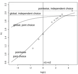
close to the pair(h1, h2) which minimized the misclassification rate. See Figure 1 for a related example
which illustrates the sample size dependence in Equation (6), and the solutions to (7)–(8).
−4 −2 0 2 4
0.8
1.0
1.2
1.4
1.6
1.8
2.0
2.2
effect of second sample size on first smoothing parameter, n2=c n1
log(c)
h1
pointwise, independent choice
global, independent choice
n1=n2 pointwise
[image:8.612.156.426.165.420.2]joint choice global, joint choice
Figure 1. Forn1 = 50, and samples fromN(0,4 2
), N(4,1)the optimal h1 (using the asymptotic equations) is shown for
various criteria, as a function of the sample sizen2=cn1. The points show the values ofh1 to minimize (over pairsh1, h2)
the average (over 20,000 simulations) squared error fˆ1(x0)−fˆ2(x0) 2
, wherex0= 2.243.
3. A Boosting algorithm for kernel density discrimination
A boosting algorithm (Shapire, 1990) repeatedly calls a “weak learner”, which is essentially a crude
classification method, M times to iteratively classify re-weighted data. The first weighting distribution
is uniform, i.e. w1(i) = 1/n, i = 1, . . . , n, whilst the mth distribution {wm(i), i= 1, . . . , n} with
(m−1)-th call. The final sequence of decision rules, δm(x), m= 1, . . . , M is summarized into a single
prediction rule which should have superior standards of accuracy.
The weighting distribution is designed to associate more importance to currently misclassified data
through some loss function. Consequently, as the number of iterations increases the ‘hard to classify’
observations receive an increasing weight. Moreover, a simple majority vote criterion (Freund, 1995),
such as the sign of PMm=1δm(x), is commonly used to combine the ‘weak’ outputs. Finally, we note
that, at present, there is no consolidated theory about a stopping rule, i.e. the value of M. This does
not seem a particularly serious drawback because boosting is often characterized by some correlation
between the training and test error.
Evidently, designing a boosted kernel classifier algorithm involves two main choices: (i) the weighting
strategy, i.e. the way to ‘give importance’ to misclassified data; (ii) the version of boosting. Other issues,
which will affect the accuracy, are: the existence of a kernel estimator and/or a bandwidth selector that
are specifically suitable for boosting.
Concerning the weighting strategy, due to its nonparametric nature, kernel discrimination lends itself
to several solutions. Two obvious criteria are: (i) locally adapting the bandwidths; and (ii) locally adapting
the mass of the kernels by associating a weight to each observation. These correspond to undersmoothing
and increasing the probability mass of kernels, respectively, for misclassified data.
A practical consideration can be helpful. Undersmoothing has the tendency to generate artificially
numerous partitions of the feature space, especially if, as it usually happens, the data are sparse; in this
case further investigation, to define an ad hoc bandwidth selector, is needed. Instead, varying the mass of
the kernel seems a directly applicable solution. In this case, the traditional kernel estimator, that gives all
observations the same mass, corresponds to the weak learner for m= 1.
Concerning an appropriate choice of boosting, we note that initial implementations of boosting used
discrete decision rules, in our case: δm(x) : R → {−1,1} (Shapire, 1990; Freund & Shapire, 1996),
whilst recently Shapire & Singer (1998) and Friedman et al. (2000) suggest more efficient continuous
mappings. In particular, Friedman et al. (2000) propose Real AdaBoosting in which the weak classifier
yields membership probabilities, in our caseδm(x) ∝pm(x ∈Πj) = ˆf2,m(x)/
n
ˆ
f1,m(x) + ˆf2,m(x)
for a fixed classΠj. Its loss system givesxi a weight proportional to
Vi=
min (p(x
i ∈Π1), p(xi ∈Π2))
max (p(xi ∈Π1), p(xi∈Π2)) 1/2
if xi is correctly classified, and proportional to Vi−1 if xi is misclassified. Besides, it is to be noted
that a continuous strong hypothesis is generated, preserving the analytical advantages of a kernel density
estimate. Because kernel methods estimate densities in order to classify, Real AdaBoost seems the natural
framework for boosting kernel discrimination , whereas discrete mappings do not employ the whole
information generated by a kernel discrimination, but only the resulting sign.
Our pseudocode for Real AdaBoost kernel discrimination (BoostKDC) is given in Algorithm 1.
Algorithm 1 BoostKDC
1. Given{(xi, Yi), i= 1, . . . , n}, initialize w1(i) = 1/n, i= 1, . . . , n.
2. Select hj, j= 1,2.
3. For m= 1, . . . , M (the number of boosting iterations)
(i) Obtain a weighted kernel estimate using
b
fj,m(x) =
X
i:Yi=j
wm(i)
hj
K x−xi hj
!
forj= 1,2.
(ii) Calculate
δm(x) = 1
2log{pm(x)/(1−pm(x))}.
where pm(x) =fb2,m(x)
. b
f1,m(x) +fb2,m(x)
(iii) Update:
wm+1(i) =wm(i)×
exp (δm(xi)) if Yi= 1
exp (−δm(xi)) if Yi= 2
4. Output
H(x) =sign ( M
X
m=1 δm(x)
)
Note that fbj,m(x) does not integrate to 1 even for m= 1; so in effect we are considering πjfj(x), with
πj = nj/n, in our estimation. Note also that we do not need to renormalize the weights because we
Considering the accuracy of the method we need to explore the overfitting phenomenon in boosting. A
weak learner overfits data when it concentrates too much on a few misclassified observations, i.e. heavily
bases the fitting on them, being unable to correctly classify them. Thus, after a value M∗
, consecutive
overfitted decision rules δM∗+1(x), δM∗+2(x). . . can worsen the performance of the final classifier. A
simple and general approach to prevent overfitting is cross-validation: M∗
is estimated by observing the
corresponding loss function when the boosting algorithm is carried out on a subsample.
However, if a flexible base learner is employed, we would expect small values ofM∗
. An illuminating
description of this phenomenon is provided by Ridgeway (2000): on a dataset where a ‘stump’ works
reasonably well, a more complex tree with four terminal nodes overfits from M = 2. Here the decision
boundary is efficiently estimated in the first step, the other steps can only overfit misclassified data
without varying the estimated boundary, so degrading the general performance. In order to reduce the
risk of overfitting, a low variance base learner is suggested, so
. . . Each stage makes a small, low variance step, sequentially chipping away at the bias.
Obviously a kernel discrimination is a flexible base learner, whatever its formulation is. Then, in a first
approximation we can adopt the criterion suggested by Ridgeway (2000) by significantly oversmoothing,
using as a bandwidth a multiple of the optimal value as obtained from classical methods.
Another regularization strategy, adopted to restrict the variance inflation due to high values of M,
is to reduce the contribution of δm(x) to H(x). This philosophy is proposed by Friedman (2001)
for a different boosting algorithm where the contribution of each step is reduced by 94%. Observing
experimental evidence, he finds an inverse relation between M∗
and the ‘Learning Rate Parameter’
(LRP), and suggests a very low LRP and a very high M. Friedman can’t justify the good practical
performances of this strategy, considering the phenomenon to be ‘mysterious’. In Real AdaBoost we can
follow this approach identifying as LRP the exponent of the probabilities ratio in the loss function. Then,
a strategy could be to replace the value 1/2 in step 3(ii) by a value 1/T with T >2. For larger values
4. The First Boosting Step (m= 2)
In this section we firstly point out an an interesting link between boosting kernel discrimination and
previous work on bias reduction in density estimation. This work was totally independent of the boosting
paradigm. Then we derive the bias of the difference estimator gˆ(x) = ˆf1(x)−fˆ2(x), involved in H(x),
at the point x0 such that f1(x0) = f2(x0) = f(x0), and show that while it is initially O(h2)- biased
(standard kernel method), boosting reduces the bias to O(h4) in the special case when h
1=h2.
4.1. RELATIONSHIP TO PREVIOUS WORK
The final classifier output by Algorithm 1 is of the form
H(x) =sign ( M
X
m=1 δm(x)
) =sign " M X m=1 1 2log (ˆ f2,m(x)
ˆ
f1,m(x)
)# .
ForM = 2 we see the decision boundary is defined by points x such that
2 X
m=1
δm(x) = 0
which is equivalent to
˜
f1(x) X
w1K
x−x
i
h1
= ˜f2(x) X
w2K
x−x
i
h2
where
w1 =
˜
f2(xi) ˜
f1(xi)
!1/2
w2 =
˜
f1(xi) ˜
f2(xi)
!1/2
and f˜j, j = 1,2 are the initial density estimates for the two groups. Thus the classification boundary can
be seen as the intersection points of two multiplicative kernel estimators.
Note that this is very similar to the variable-kernel density estimator of Jones et al. (1995):
b
f(x) =fbb(x) 1 n n X i=1 b f−1
b (xi) 1
hK
x−x
i
h
, (11)
where fbb is the classical estimator with the bandwidth b. We can see that Equation (11) is simply the
product of an initial estimate, and a (re-)weighted kernel estimate, with the weights depending on the
the leading bias in fbb(x) should cancel with the leading bias in fb(xi) and their paper showed that this
was an effective method of nonparametric density estimation. In its simplest form, b = h. A recent
semiparametric modification of this method was proposed by Jones et al. (1999).
Di Marzio & Taylor (2004a) showed that kernel density estimates could be directly boosted by
defin-ing a loss function in terms of a leave-one-out estimate (see Silverman, 1986, p. 49), and they established
a link between this version of boosting and the bias-reduction technique of Jones et al. (1995).
4.2. BOOSTINGREDUCES THEBIAS
In order to gain some insights into the behaviour of boosting we consider a population version: this
corresponds to the situation in which there is an infinite amount of data, but the smoothing parameter is
bounded away from 0. We examine the weights and classifiers for learners which are “weak” in the sense
that our estimate off(x) is given by:
b
fj,m(x)∝
Z 1
hj
K x−y hj
!
wj,m(y)fj(y)dy forj= 1,2.
The first approximation in the Taylor series expansion (which we use for the initial estimate, whenm =
1) is
ˆ
f(x) =f(x) +h2f′′
(x)/2 (12)
for someh >0. So the initial classifier then uses
δ1(x) ∝ 1
2
n
log ˆf2,1(x)−log ˆf1,1(x) o = 1 2 " log f 2(x) f1(x)
+h
2 2f
′′
2(x)
2f2(x) −h
2 1f
′′
1(x)
2f1(x)
+O(h41) +O(h42)
# .
Thus atx0 we have a bias given by:
∆1(ˆg(x0)) = h2
2f
′′
2(x0)−h21f
′′
1(x0)
4f(x0)
. (13)
which is of order O(h2).
We then obtain, form= 2
ˆ
f1,2(x) ∝ Z 1
h1 K
x−y
h1
fˆ 2,1(y)
ˆ
f1,1(y) !1/2
f1(y)dy (14)
ˆ
f2,2(x) ∝ Z 1
h2 K
x−y
h2
fˆ 1,1(y)
ˆ
f2,1(y) !1/2
By substituting Equation (12) into Equations (14) and (15), expanding in a Taylor series and making the
change of variable we eventually obtain an approximation up to terms of order h2i, i= 1,2:
ˆ
f1,2(x) = (f1(x)f2(x))1/2 "
1 +
( f′′
2(x)
4f2(x)
+ f
′
1(x)f
′
2(x)
4f1(x)f2(x) −(f
′
2(x))2
8f2 2(x)
−(f
′
1(x))2
8f2 1(x)
) h21
+f
′′
2(x)
4f2(x) h22
ˆ
f2,2(x) = (f1(x)f2(x))1/2 "
1 +
( f′′
1(x)
4f1(x)
+ f
′
2(x)f
′
1(x)
4f1(x)f2(x) −(f
′
1(x))2
8f12(x) − (f′
2(x))2
8f22(x)
) h22
+f
′′
1(x)
4f1(x) h21
.
From this we can compute up to terms of order h3j, j= 1,2:
δ2(x) =
1 2
"
+(h
2 1−h22)
8
f′
1(x) f1(x)
−f
′
2(x) f2(x)
2
+(h
2 2+h21)
4
f′′
1(x) f1(x)
−f
′′
2(x) f2(x)
#
which gives an updated classifier which usesδ1(x) +δ2(x). Thus atx0 we have bias given by
∆2(ˆg(x0)) =
∆1(ˆg(x0))
2 +
h2 2f
′′
1(x0)−h21f
′′
2(x0)
8f(x0)
+ (h21−h22)
f′
1(x0)−f2′(x0)
4f(x0) 2
If we now set h1 =h2 we see that∆2(ˆg(x0)) =O(h4) so boosting gives bias reduction. That boosting
reduces the bias comes as no surprise, but it is somewhat counter-intuitive that the bias reduction is
enhanced by taking equal smoothing parameters.
Simple closed form expressions for the variance have eluded us, but we believe that, in common with
other applications of boosting, the variance will increase rather slowly with M.
5. Numerical and Simulation Experiments
We will not address the issue of automatic bandwidth selection for kernel classification. Even in the
regular (non-boosting) situation, this is not straightforward. Cross-validation could be a possible solution
to finding good pairs (h1, h2), but in our simple experiments, the surface often has local minima, in
which the loss, given by the number misclassified observations, is a discrete function. However, it is worth
reiterating that the automatic or data-based choices of smoothing parameter that have been developed for
Our case studies consist of four simple discrimination problems. The models are: two gaussian cases,
with equal or different variance (M1, M2); a limited support case (M3) and a heavy-tailed case (M4). In
particular: M1 := N 0,42, N 4,12, M2 := N 0,32, N 4,32, M3 := N 4,12,exp (2) and
M4:=N 4,12, t(2).
As our loss function we will consider the root mean squared error of the estimatorxˆ0 =x: ˆf1(x) =
ˆ
f2(x), calculated on B samples with equally sized groups (with n1=n2):
\
RMSE(ˆx0) = ( PB
b=1(ˆx0,b−x0)2 B
)1/2 .
The reasons for focussing on xˆ0 are twofold. Firstly, the above risk criterion allows us to examine the
behaviour of the two contributions: namely the bias and variance of the estimator xˆ0. Secondly, it
re-enforces the fact that the source of inflated error rates is due to poor estimation of the decision boundaries.
Connections between x0 and the error rate are further explored in Friedman (1997).
The secondary solutions for x0, where they existed, contribute very little to the error rate, and
so were simply ignored for simplicity. Note that in some cases the secondary solution was such that
f′′
1(x0)f2′′(x0)>0which requires special attention; see Equation (13) and the discussion in Section 2.2.
A further potential problem is that, particularly for small choice ofh, we could get multiple solutions to
ˆ
f1(x) = ˆf2(x) in the vicinity of x0. However, for the values of h considered here, this never occurred
in any of our simulations.
In our simulation studies two main aspects are explored. In subsection 5.1 we consider using separate
estimation, a simple benchmark for kernel density discrimination. Obviously, a discrimination based on
independent estimations uses J independent estimates which leads to a partition of Rgenerated on the
basis of thex0s as defined above. The performance of a number of current estimators are compared. Here
the end is threefold: firstly investigating if there is an estimator that behaves better than others in
classifi-cation (as opposed to density estimation); secondly, to establish whether the bias-reduction properties of
higher-order bias kernel methods transfer to the estimation ofx0; thirdly, benchmark accuracy values are
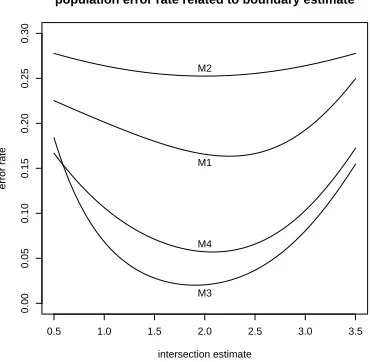
established for the subsequent analysis. Figure 2 shows the relationship between the intersection point
and the error rate for the models used in the simulations. It appears that the intersection point will give
more sensitivity in assessing the performance of our methods. In subsections 5.2–5.3 we investigate the
0.5 1.0 1.5 2.0 2.5 3.0 3.5
0.00
0.05
0.10
0.15
0.20
0.25
0.30
population error rate related to boundary estimate
intersection estimate
error rate
M1 M2
[image:16.612.201.386.59.240.2]M3 M4
Figure 2. Relationship between the error rate and the estimate ofx0 for the four models considered.
behaviour to check what we formally found for M = 2. In subsection 5.3 the consequences of various
tuning choices of parameters, such as the bandwidths and the number of iterations to be carried out, are
explored.
5.1. SEPARATEESTIMATION
We have compared the performances of five estimators: the linear discriminant (LD) the classic kernel
estimator (CK) given by Equation (1), two adaptive estimators: the algorithms by Abramson (1982) (AB)
and Jones et al. (1995) (JLN), and finally the jackknifed higher order kernel (HO). JLN was discussed in
Section 4; a brief description of AB and HO follows.
Consider the general formulation
b
f(x) = 1
n
n
X
i=1
1
h(xi)
K
x−x
i
h(xi)
,
where there is a different bandwidth for every sample element. Due to verified practical performance and
some optimal analytic properties, a good choice is to take h(xi) proportional tofe(xi)−1/2, where feis
a pilot estimator of f (Abramson, 1982). This estimator has been closely studied and some theoretical
drawbacks have been found (Terrell & Scott, 1992; Hall & Turlach, 1999); however Abramson’s solution
is still very appealing for its simplicity and effectiveness. A higher order kernel estimator uses a kernel
Concerning the order of the kernel, there is general agreement that good improvements can often be
obtained with k = 4. One of the principal reasons why they do not have a greater usage in practice
is because they take negative values, so the resultant estimate is not itself a density. In a discrimination
setting, this defect is not particularly serious, because we are not primarily interested in a density estimate.
In fact, our goal is to determine whether f1(x) > f2(x) for given x. However, other drawbacks, such
as a difficult choice of bandwidth and the poor enhancements for reasonably sized samples (Marron &
Wand, 1992; Jones & Signorini, 1997), could be still valid in a discrimination framework. Following
Jones & Signorini (1997), we consider the generalized-jackknife estimator given by
b
f(x) = 1
n
n
X
i=1
1
hK(4)
x−x
i
h
,
with
K(4)(u) =
µ4(K)−µ2(K)u2K(u)
µ4(K)−µ2(K)2
whereµj(K) =R xjK(x)dx.
Concerning the implementation details, we have used two step versions of AB and JLN. This is
because in both cases the second step effects the major bias deletion, while the residual bias is slowly
reduced across the successive steps at the expense of a significant variance inflation. Moreover we have
used a normalized version of JLN.
We have used the simple normal scale ruleh= 1.06σnb −1/5
for two reasons. From a population point
of view, we have almost always unimodal symmetric populations, the only exception being the
exponen-tial population that, however, is not particularly concentrated near the boundary. From the estimator’s
point of view, AB and JLN, because of their iterative nature, are robust to the bandwidth selection step,
moreover, higher order kernel theory is not particularly developed for bandwidth selection. We use small
sample sizes to indicate the effectiveness of the asymptotic arguments with real datasets.
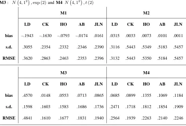
The bias, s.d. and RMSE of the xˆ0’s for ni = 50, i = 1,2, and B = 500 are reported in Table I.
In problem M1 the O(h4)-biased estimators perform drastically better than CK. A large bias reduction
(around 90%) is obtained without a variance inflation. AB and JLN exhibit very similar accuracy values,
while HO reduces the bias more modestly (around 51%) but exhibits the smallest variance. In the
estima-tion of problem M2 there is not a bias problem, but AB is a little more stable than the other estimators,
Table I. Accuracy values for 5 separate estimations of x0 such that f1(x0) = f2(x0) with
ni= 50, i= 1,2. The models for the fi are: M1 N 0,4
2
, N 4,12
, M2 N 0,32
, N 4,32
,
M3: N 4,12
,exp (2)and M4 N 4,12
, t(2)
M1 M2
LD CK HO AB JLN LD CK HO AB JLN
bias –.1943 –.1630 –.0793 –.0174 .0161 .0315 .0033 .0073 .0101 .0011
s.d. .3055 .2354 .2332 .2346 .2390 .3116 .5443 .5349 .5183 .5457
RMSE .3620 .2863 .2463 .2353 .2396 .3132 .5443 .5350 .5184 .5457
M3 M4
LD CK HO AB JLN LD CK HO AB JLN
bias .4570 .0148 .0553 .0713 .0865 .0685 .0899 .1355 .1069 .1184
s.d. .1598 .1603 .1583 .1686 .1736 .2471 .1718 .1812 .1854 .1909
RMSE .4841 .1610 .1677 .1831 .1940 .2564 .1939 .2263 .2140 .2246
since it is optimal for such distributions. Curiously, in problem M3 and M4 CK gives the best results. In
problem M3, AB and JLN perform so poorly because their pilot estimation is O(h) biased near zero,
HO performs similarly to CK. In problem M4, due to the sparseness of the data in the tails of the t
distribution, larger sample sizes are required in order to make effective the properties of O(h4)-biased
estimators. However, it should be noted that in the models M3 and M4 there is a nearly symmetric pattern
in a wide neighbourhood of x0. Obviously LD performs very poorly when the population variances are
quite different.
5.2. TWOBOOSTINGITERATIONS
In this subsection we have implementedBoostKDCusing the standard kernel density estimator, given
by Equation (1), and the normal scale rule to select h= 1.06ˆσn−1/5
. This very simple automatic choice,
which is well-known to oversmooth, should make clear the effect of boosting and should satisfy the
non-normal data. Our objective was to observe the reduction in bias, theoretically derived in Section 4.2,
and to confirm that a common smoothing parameter (h1 = h2 = h) was asymptotically superior to
separate smoothing parameters. So two bandwidth selection strategies were adopted: the separate and
the common strategy. TwoBoostKDCestimators result: one using separate bandwidths, with first step a
classical kernel (CK), and second step referred to as 2KBs; a second estimator where the same bandwidth
hKB = (h1×h2)1/2 is employed to estimate both f1 and f2 (1KBc and 2KBc). We have chosen the
selector hKB for its simplicity and because it will again weaken the learner by oversmoothing. However,
in the light of theory of Section 4 we note that the bandwidth selection task should not be crucial for
2KBc, provided that the unique bandwidth employed is able to control the effects of higher order bias
terms. Actually, we observed numerical evidence to support this hypothesis.
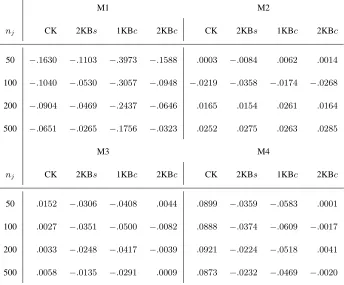
The numerical experiment consists of the estimation of models M1–M4 and the three sample sizes:
[image:19.612.127.471.387.672.2]50, 100, and 500. The accuracy values of CK, 2KBs, 1KBc and 2KBc are contained in Table II.
Table II. Bias of (i) the classical estimator (CK) and the second boosting step ofBoostKDC
with separate (2KBs) bandwidths and (ii) common bandwidth selection with one (1KBc) and
two iterations (2KBc) ofBoostKDC. Different sample sizes for each of models M1–M4.
M1 M2
nj CK 2KBs 1KBc 2KBc CK 2KBs 1KBc 2KBc
50 −.1630 −.1103 −.3973 −.1588 .0003 −.0084 .0062 .0014
100 −.1040 −.0530 −.3057 −.0948 −.0219 −.0358 −.0174 −.0268
200 −.0904 −.0469 −.2437 −.0646 .0165 .0154 .0261 .0164
500 −.0651 −.0265 −.1756 −.0323 .0252 .0275 .0263 .0285
M3 M4
nj CK 2KBs 1KBc 2KBc CK 2KBs 1KBc 2KBc
50 .0152 −.0306 −.0408 .0044 .0899 −.0359 −.0583 .0001
100 .0027 −.0351 −.0500 −.0082 .0888 −.0374 −.0609 −.0017
200 .0033 −.0248 −.0417 −.0039 .0921 −.0224 −.0518 .0041
We expect that data from Problem M1 generate heavily biased estimates because f1 and f2 exhibit
quite different curvatures near x0. However, in correspondence of each sample size our boosting
algo-rithms are clearly less biased than CK. Comparing boosting algoalgo-rithms, we note that 2KBc increases its
accuracy values faster than 2KBsasnincreases. Specifically, comparing the bias magnitudes atn= 50,
we have −80%for 2KBcand −75% for 2KBs; while for theSDrespectively −65% versus −59%.
In problem M4, because of the presence of a heavily tailed distribution, the bias of CK does not
decrease for large samples, boosting shows an even more marked ability to reduce it. Here 2KBc is
substantially unbiased, while 2KBs is decidedly less biased than CK, in fact the bias ratios are0.40 for
n= 50and 0.27 for n= 500. Moreover, for n= 500 2KBc appears more stable than CK.
Concerning models M2 and M3, in the previous section we observed the substantial unbiasedness of
CK forn= 50because of the perfect or approximate symmetry exhibited near x0. As a consequence, we
expect our boosting will not help. Anyway, for this latter reason M2 and M3 constitute a good benchmark
in order to measure the overfitting of our two-step algorithms.
Overall, comparing Tables I and II, we can see that boosting does have a bias-reduction property
which, in some cases, mimics those of the higher-order kernel methods. On the whole, if boosting CK
works well, then the use of a common bandwidth seems preferable. Finally, an impressive feature of
BoostKDCis that it appears robust to non-regular shapes of the populations.
5.3. MOREBOOSTINGITERATIONS
In this subsection we explore the performance of boosting when more than two iterations are carried
out. According to the boosting principles we expect an initial progressive bias reduction and a modest
variance inflation. We expect that after a number of steps both variance and bias will start to increase and
from around there we will observe overfitting.
Our objective is to explore the way in which the optimal choice of smoothing parameter varies as
the number of iterations increases, and to investigate how many boosting iterations are effective. As
noted, boosting cannot work for problem M2 since the distributions are symmetric and so there is no
bias. In this equal variance Normal setting a linear discriminant xˆ0 = ( ¯x1+ ¯x2)/2 is optimal and this
each distribution we simulate 500 samples with n1 =n2 = 50 and for common smoothing parameters
(h1 =h2) in an appropriate range we calculate xˆ0 for m = 1,2, . . .. Based on these 500 numbers we
then estimate the bias and variance which would be achieved for each combination of m and h. Results
for data model M1 are shown in Figure 3, in which we show the bias-variance trade-off. We can see that
the bias continues to reduce by boosting for 4 iterations or more, and then a larger value ofh can be used
to reduce the variance. In terms of RMSE, there is little improvement beyond 7 iterations, after which
these values are almost entirely dominated by the variance component. The RMSE results for models M3
0.5 1.0 1.5 2.0
0.00
0.10
0.20
0.30
M1 Boosting: Bias vs m, h
smoothing parameter
Bias
M=1
M=13
0.5 1.0 1.5 2.0
0.15
0.20
0.25
0.30
M1 Boosting: SD vs m, h
smoothing parameter
Standard Deviation
[image:21.612.59.520.264.485.2]M=1 M=2
Figure 3. Effect of number of boosting iterations and the smoothing parameter on bias and variance of estimation ofx0. Left: Bias; Right: Standard deviation form= 1, . . . ,13as a function of h. The points, which are shown on both panels, are the
optimal (overh) root mean squared error values for each choice ofm.
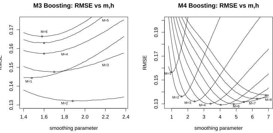
and M4 are shown in Figure 4 and the behaviour is somewhat similar in each: as the number of boosting
iterations increases the optimal choice of smoothing parameter also increases. Whereas for model M1 the
RMSE corresponding to this optimal choice of h continued to decrease slowly up to m= 13 iterations,
1.4 1.6 1.8 2.0 2.2 2.4
0.13
0.14
0.15
0.16
0.17
M3 Boosting: RMSE vs m,h
smoothing parameter
RMSE
M=1
M=2
M=3 M=4
M=5
M=6
1 2 3 4 5 6 7
0.13
0.15
0.17
0.19
M4 Boosting: RMSE vs m,h
smoothing parameter
RMSE
M=1
M=2 M=3
M=4 M=6 M=7
[image:22.612.64.518.57.278.2]M=8
Figure 4. Effect of number of boosting iterations and the smoothing parameter on the root mean squared error (RMSE) of estimation ofx0. Points show minima for eachM. Left: Model M3; Right: Model M4 as a function ofh.
6. Conclusions
The goal of this paper was to consider some theoretical aspects and solutions in kernel density
discrim-ination. Concerning the algorithm BoostKDC, we have demonstrated the utility of boosting in kernel
density classification both theoretically and for finite samples. However, obtaining explicit formulae for
the variance has proved elusive, and it is not theoretically clear the way in which the bias reduction works
for more than two steps.
In many situations, the intersection point x0 will not be unique, and, since the estimation at such
x0 is critical, adaptive smoothing parameters are likely to perform much better than global smoothing
parameters. In particular, if f′′
1(x0)f2′′(x0)>0 then a much larger smoothing parameter is required; see
Equation (13). In practical applications, it would be necessary to obtain a rule to enable an appropriate
data-based choice of smoothing parameter h and a regularization technique (appropriate choice of M)
should also be a matter for concern. In general, it appears that the larger the choice of M, the larger is
the optimal smoothing parameter.
A further issue which requires more investigation is the Learning Rate Parameter1/T (= 1/2in step
slower, reducing the overfitting phenomenon. In fact, values of T a little larger than 2 often generate
much more efficient estimates. A further method to ameliorate overfitting would be to use shrinkage
(B ¨uhlman & Yu, 2003). A final methodological point is establishing if the use of boosting weights
{wi,m, i = 1, . . . , n, m = 1, . . . , M} could be incorporated into the calculation of the bandwidth, so
achieving a step-adaptive bandwidth.
The simple nature ofBoostKDC allows a straightforward extension to the multidimensional case
which is examined by Di Marzio & Taylor (2004b) who show the effectiveness of boosting in reducing
the error rate on both simulated and real data.
Acknowledgement: We are grateful to two anonymous referees for detailed and helpful comments that
led to significant improvements in this paper.
References
Abramson, I.S. (1982). On bandwidth variation in kernel estimates — a square root law. Annals of
Statistics, 9, 127–132.
B ¨uhlmann, P. & Yu, B. (2003). Boosting with L2-Loss: regression and classification. Journal of the
American Statistical Association 98, 324–449.
Di Marzio, M. & Taylor, C.C. (2004a). Boosting Kernel Density Estimates: a Bias Reduction Technique?.
Biometrika, 91, 226–233.
Di Marzio, M. & Taylor, C.C. (2004b). On learning kernel density methods for multivariate data: density
estimation and classification. submitted for publication.
Freund, Y. (1995). Boosting a weak learning algorithm by majority. Information and Computation. 121,
256–285.
Freund, Y. & Shapire, R. (1996). Experiments with a new boosting algorithm. In Machine Learning:
Pro-ceedings of the Thirteenth International Conference, Ed. L. Saitta, pages 148–156. Morgan Kauffman,
Friedman, J. H. (1997) On bias, variance, 0/1-loss, and the curse of dimensionality. J. Data Mining and
Knowledge Discovery, 1, 55–77.
Friedman, J.H. (2001). Greedy function approximation: A gradient boosting machine. Annals of
Statistics, 29, 1189–1232.
Friedman, J.H., Hastie, T. & Tibshirani, R. (2000). Additive logistic regression: a statistical view of
boosting (with discussion). Annals of Statistics, 28, 337–407.
Habbema, J.D.F., Hermans, J. & van der Burgt, A.T. (1974). Cases of doubt in allocation problems.
Biometrika, 61, 313–324.
Hall, P., Hu, T.-C. & Marron, J.S. (1995). Improved variable window kernel estimates of probability
densities. Annals of Statistics, 23, 1–10.
Hall, P. & Turlach, B. (1999). Reducing bias in curve estimation by the use of weights. Computational
Statistics and Data Analysis, 30, 67–86.
Hall, P. & Wand, M.P. (1988). On nonparametric discrimination using density differences. Biometrika,
75, 541–547.
Hand, D.J. (1982). Kernel Discriminant Analysis. Research Studies Press, Chichester.
Hastie, T., Tibshirani, R. & Friedman, J. (2001). The Elements of Statistical Learning. Springer, New
York.
Jones, M., Linton, O. & Nielsen, J. (1995). A simple bias reduction method for density estimation.
Biometrika, 82, 327–338.
Jones, M.C. & Signorini, D.F. (1997). A comparison of higher-order bias kernel density estimators.
Journal of the American Statistical Association, 92, 1063–1073.
Jones, M.C., Signorini, D.F. & Li, H.N. (1999). On multiplicative bias correction in kernel density
estimation. Sankya, 61, 1–9.
Michie, D., Spiegelhalter, D.J. & Taylor, C.C. (1994) Machine Learning, Neural and Statistical
Classification. Ellis Horwood, Chichester.
Ridgeway, G. (2000). Discussion of “Additive logistic regression: a statistical view.” Annals of Statistics,
28, 393–400.
Shapire, R.E. & Singer, Y. (1998). Improved boosting algorithms using confidence-rated prediction. In
Proceeding of the eleventh annual conference on computational learning theory.
Silverman, B.W. (1986). Density Estimation for Statistics and Data Analysis. Chapman and Hall,
London.
Terrell, G.R. Scott, D.W. (1992). Variable kernel density estimation. Annals of Statistics, 20, 1236–1265.
Wand, M.P. & Jones, M.C. (1995). Kernel Smoothing. Chapman and Hall, London.
Wright, D.E., Stander, J. & Nicolaides, K. (1997). Nonparametric density estimation and discrimination