Adaptive control of nonlinear dynamical systems using a model reference approach

model reference approach

.

White Rose Research Online URL for this paper:

http://eprints.whiterose.ac.uk/79681/

Version: Accepted Version

Article:

Wagg, D.J. (2003) Adaptive control of nonlinear dynamical systems using a model

reference approach. Meccanica, 38 (2). 227 - 238. ISSN 0025-6455

https://doi.org/10.1023/A:1022854621106

Reuse

Unless indicated otherwise, fulltext items are protected by copyright with all rights reserved. The copyright exception in section 29 of the Copyright, Designs and Patents Act 1988 allows the making of a single copy solely for the purpose of non-commercial research or private study within the limits of fair dealing. The publisher or other rights-holder may allow further reproduction and re-use of this version - refer to the White Rose Research Online record for this item. Where records identify the publisher as the copyright holder, users can verify any specific terms of use on the publisher’s website.

Takedown

If you consider content in White Rose Research Online to be in breach of UK law, please notify us by

Adaptive control of nonlinear dynamical systems using

a model reference approach

David J. Wagg

Department of Mechanical Engineering, University of Bristol, Queens Building, University Walk, Bristol BS8 1TR, U.K.

May 3, 2013

Keywords: Nonlinear dynamics; adaptive control; model reference

1. Introduction

Control of systems which exhibit nonlinear dynamical behavior, par-ticularly chaos, has been an active area of interest in recent years following the work of Ott, Grebogi, & Yorke (1990). In addition to this approach, nonlinear systems which exhibit chaotic dynamics have also been controlled using a more standard control engineering approach including techniques such as feedback linearization and adaptive con-trol (Di Benardo, 1996). Of these approaches, adaptive concon-trol is often most useful in a practical engineering environment, as it requires only a limited knowledge of the plant structure and parameters. When a reference model is used, adaptive controllers can also be applied to systems where the details of the plant cannot be fully known a priori

or vary with time. Using these type of algorithms without knowledge of plant parameters, such that we assume zero initial conditions for the controller gains, has become known as the “minimal control synthesis” approach (Stoten, 1993). Basing adaptive control schemes on a refer-ence model enables the system to be controlled to behave like the model itself. This type of approach is applied to a wide range of systems, but is based primarily on linear control theory, as the required model is usually a linear one. In this type of system, the effect of nonlinearities and/or disturbances is compensated for by the adaptive nature of the controller.

In this paper we review linear reference model adaptive control, in particular the “minimal control synthesis” approach. We consider how linear adaptive controllers are designed using both hyperstability and Lyapunov stability analysis. We then discuss using model refer-ence adaptive controllers to control systems which exhibit nonlinear dynamical behaviour.

nonlinearity is “small” then standard linear model reference control can be applied. A second example, which is often found in synchroniza-tion applicasynchroniza-tions, is when the nonlinearities in the plant and reference model are identical. Again we show that linear model reference adaptive control is sufficient to control the system.

Finally we consider controlling more general nonlinear systems. For these systems we discuss how adaptive feedback linearization control can be used to control scalar systems. As an example we use two systems with chaotic behaviour; the Lorenz and Chua systems. The Lorenz system is used as a reference model and a single coordinate from the Chua system is controlled to follow one of the Lorenz system coordinates. Some examples of using feedback linearization to control mechanical systems are given by Goodwine & St´ep´an (2000) who con-sider control of towed wheels, Lin & Lin (2001) who concon-sider spacecraft control and Menson & Ohlmeyer (2001) who consider missile guidance and autopilot systems.

2. Theoretical formulation for general linear systems

We begin by considering the general linear state space formulation for model reference adaptive control. The state equation can be written in the form

˙

x(t) =Ax(t) +Bu(t) +d(t), (1) where x is the state variable vector, u the control signal vector, A represents the linear dynamics of the plant, B the linear dynamics of the controller and d(t) is a disturbance term.

In general we consider a controller which uses both the state vari-ables and the reference signal, factored respectively by the adaptive gains K(t) andKr(t), such that

u(t) =K(t)x(t) +Kr(t)r(t), (2)

wherer(t) is the reference (demand) signal,K(t) is the feedback adap-tive gain andKr(t) the feed forward adaptive gain. This type of

assump-tion on the structure of the control signal requires that the demand sig-nal r has sufficient persistence of excitation (Sastry & Bodson, 1989).

Substituting equation (2) into equation (1) gives

˙

x=Ax+B(Kx+Krr) = (A+BK)x+BKrr+d(t). (3)

The plant is controlled to follow the output from a reference model with known dynamics

˙

wherexm is the state of the reference model andAm andBm are linear

reference equivalents of A and B.

We need to monitor the performance, or effectiveness of the con-troller, and this is done using the error signalxe=xm−x. The objective

of the control algorithm is xe → 0 ast→ ∞. We can reformulate the

dynamics of the system as the error dynamics

˙

xe=Amxe+ (Am−A−BK)x+ (Bm−BKr)r−d(t). (5)

Comparing equations (4) and (3), we can see that for exact matching between the plant and the reference model, the following relations hold

A+BK∗ _=Am

BK∗

r =Bm (6)

where ()∗ _{denotes a constant value.}

Assuming all matrix (pseudo) inverses exist we can obtain expres-sions (generally known as the Erzberger conditions (Khalil, 1992) for the gain values as

K∗_=B−1

(Am−A)

K∗

r =B−

1

Bm . (7)

However, one of the main aims of model reference adaptive control is to operate without explicit knowledge of the plant parameter values, which in this case are the matrices A and B. In fact one of the most significant advantages of this type of controller is that it can operate without explicit values for the matricesAandB. As a result we cannot usually solve equation (7), but we can use it to express the matrix terms given in equation (5), as

B(K∗_{−K) = (Am−A−BK)}

B(K∗

r −Kr) = (Bm−BKr) . (8)

Now we define functions which represent the variation of the adaptive gains K(t) andKr(t) from the exact matching solution valuesK∗ and

K∗

r. Let

φ(t) = (K∗_−K(t))

ψ(t) = (K∗

r −Kr(t)), (9)

then using equation (6) and (9) we can rewrite equation (5) as

˙

xe=Amxe+B(φx+ψr)−d(t) (10)

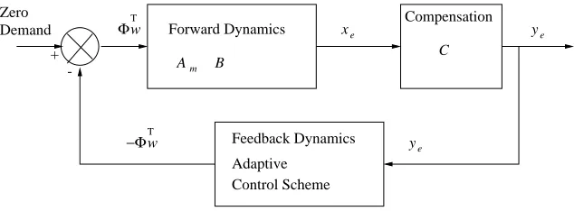
(Banks, 1986, Khalil, 1992). This can be further abbreviated by defin-ing Φ(t) ={φ, ψ}T _{and w(t) ={x, r}}T_{, such that}

˙

C

x y

Φ

w w

−Φ

e e

Zero Demand

A_m B

Forward Dynamics

Adaptive Control Scheme

y_e

+

-Compensation

Feedback Dynamics T

T

Figure 1. Schematic representation of error dynamics as a feedback system.

Thus the error system can be reduced to a single ordinary differential equation, with distinct linear and nonlinear parts. Note by denoting k={K, Kr}T and k∗ ={K∗, Kr∗}T, we can write

Φ = (k∗_{−k). (12)}

In this formulation Φ can be thought of as a gain or parameter error: i.e. the difference between the exact matching conditions and the current adaptive gain values.

3. Controller design

In general, for linear systems, we wish to design an adaptive controller for as wide a class of systems{A, B}as possible. Of primary importance is the overall stability of the system. Thus controller design is usually approached with some stability criteria in mind. For adaptive systems there are two commonly used stability criteria; Lyapunov stability and hyperstability. We will first consider hyperstability, often referred to as the Popov Criteria (see Banks (1986) for a derivation). In both stability analyses we exclude the disturbance term d(t) which is assumed to be small and bounded, and therefore to be a robustness not a stability issue (Sastry & Bodson, 1989).

A key feature of the hyperstability criteria is that the system can be divided into “blocks”, each of which can be proved stable inde-pendently. This technique can greatly simplify the stability problem for a wide class of control systems (Landau, 1979). In the case of the model reference system, we spilt the system into a feed forward block and a feedback block (e.g. see Stoten & Benchoubane (1990)). This is illustrated schematically in figure 1.

xe= 0. The feed forward dynamic block is represented by equation (11)

and gives an output error signalxe. In the general case we assume that

the error signal is compensated via the constant linear matrix C such that ye = Cxe. C can be chosen to ensure the stability of the feed

forward block (Landau, 1979). This compensated error is used in the adaptive control scheme which is represented as a feedback block in figure 1. The control scheme gives an output of −Φ(t)w(t) which is added to the demand in the feedback loop.

Having split the system into forward and feedback blocks, we use hyperstability to show the stability of each block. The forward dynam-ics are linear, and we can show that {Am, B, C} form a hyperstable

block using the Lyapunov equation

AT_mP+P Am =−Q, (13)

whereC =BT_{P andQis positive definite. In other words the transfer}

functionC(sI−A)−1_{Bmust be strictly positive real (SPR). This is now}

referred to as the Kalman-Yacoubovich-Popov Lemma, and a proof can be found in Sastry 1999.

For the feedback block, we use the integral inequality

Z t

t0

ye(t)(−Φ(t)Tw(t))dt≥ −γ

2

, (14)

where γ is a finite constant. By differentiating, equation (14) can be expressed as

−yeΦTw(t)≥0. (15)

from which we can see that the solution ΦT _=−C

1yewT,C1>0 satis-fies the inequality. This is effectively a simple proportional controller, however we need a controller which maintains a gain value as ye→ 0.

Adding an integral term will allow the adapted value to remain when ye= 0. Thus we adopt an adaptive gain of the form

k(t) =C1yew+C2

Z t

t0

yewdt, (16)

where C1 and C2 are arbitrary positive constants. By denotingk(t) = k1+k2 as the sum of the proportional and integral parts, we note that k1 = (C1/C2) ˙k2 and that Φ = (k∗ −(k1+k2)) and −k1 = −C1y_ew. Now we partition Φ such that Φ = Φα+ Φβ, where Φα =k∗−k2 and Φβ = −k1. From this we note that Φ_β = −k1 = (C1/C2) ˙Φ_α (k∗ is a constant so it goes to zero when differentiated). Then substituting these relations into equation (14) gives firstly

−

Z t

t0

ye(t)(Φα+ Φβ)w(t)dt≥ −γ

2

then, substituting−yew=−k1/C1= Φβ/C1 = ˙Φα/C2 we can write

1 C2

Z t

t0

Φα˙Φαdt+

1 C1

Z t

t0

ΦβΦβdt≥ −γ

2

. (18)

The second integral term is now always greater than zero providing C1 >0. For the first integral term we have that,

1 C2

Z t

t0

Φα˙Φα≥ −

1 2C2

Φα(t0)TΦ_α(t0)≥ −γ 2

, (19)

using the relation

Z t

t0

f(t) ˙f(t)dt= 1 2(f

2

(t)−f2(t0))≥ − 1 2f(t0)

2

, (20)

(f(t) scalar). Thus the hyperstability condition is satisfied (Popov, 1973). For general model reference adaptive control, the gains are defined setting C1 =β and C2 =α such that

k=α

Z t

0

yew(t)dt+βyew(t). (21)

Equation (21) gives an expression which computes the adaptive gain values, k(t), from timet= 0 to an arbitrary timet. However, α andβ need to be selected in advance, and clearly have a significant influence on the rate of adaption. As yet there is no theoretical approach to choosing values for α andβ.

3.1. Lyapunov stability analysis

An alternative stability criteria is Lyapunov stability, see for example Sastry (1999). Here we consider the analysis of a single input single output system with error dynamics

˙

xe=−amxe+bΦTw (22)

wherexe,am >0 andbare scalar. As with the hyperstability proof, we

define Φ = Φα+ Φβ. To prove the stability of the system, we select a

trial Lyapunov function of

V = x 2

e

2 + b 2αCΦ

T

αΦα (23)

(Sastry, 1999). Note also we are only using Φα not Φ to define the

Lyapunov function.

Essentially, we must show that the derivative of the Lyapunov func-tion ˙V is negative definite for all initial values and for all time. The derivative of V is given by

˙

V =xex˙e+

b αCΦ

T

α˙Φα. (24)

Substituting for ˙xe using equation (22) gives

˙

V =−amx

2

e+xeb(Φα+ Φβ)Tw+

b αCΦ

T

α ˙Φα. (25)

The key step is now to substitute for ˙Φα, which from the previous

section, equation (18), can be expressed as ˙Φα =−αyew, which gives

˙

V =−amx2e−xebΦTβw. (26)

Finally substituting for Φβ gives

˙

V =−amx

2

e−βCx

2

ewTw, (27)

which for am, β, C > 0 is always negative definite. A matrix version

of this type of analysis can be found for example in Landau (1979) or Sastry (1999). In addition, an interesting variation of this type of anal-ysis for non-quadratic Lyapunov functions is described by Rao (1998). A comparison between hyperstability and Lyapunov stability analysis is given in Narendra & Valavani (1980).

4. Nonlinear Systems

We now consider the case when both the plant and reference model have a nonlinear structure (without a disturbance) of the form

˙

x(t) =f1(x, t) +g1(u, t), ˙

xm(t) =f2(xm, t) +g2(r, t),

(28)

the linear system. This approach can be applied to systems where the term d(t) remains small and bounded such that the linear stability analyses can be applied. For example we can use this approach to control a range of nonlinear systems to behave in a linear way providing the nonlinearity remains small.

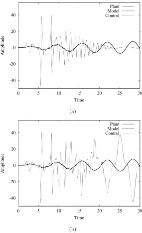
Example 1: Nonlinearity small and bounded

In this case h2 = 0, and d(t) =h1. So, if we consider the case where a linear reference model is used, and the plant is a Duffing type oscillator

¨

x+δx˙+σx−ǫx3 =u(t) ¨

xm+δx˙m+σxm =qcos(ωt). (29)

then for small ǫ the Duffing oscillator can be controlled to track the output of the reference model. A numerical example of this using MCS control is shown in figure 2, where δ = 0.1 and σ = q = ω = 1. In figure 2 (a) we show the linear case, ǫ = 0 where the plant tracks the model output after approximately 15 seconds. In figure 2 (b) we show the case when ǫ = 0.1, where again the plant tracks the model output after approximately 15 seconds. However in this case the effect of the nonlinearity means that the control signal is significantly larger in amplitude after tracking occurs than in the linear case. For this particular example linear control works up to approximately ǫ = 0.5 after which the tracking deteriorates significantly. However, by decreas-ing the numerical integration timestep and increasdecreas-ing controller gain values it is possible to simulate stable control for larger ǫ values.

4.1. A general formulation for nonlinear systems

For general nonlinear functions we can write the error dynamics as

˙

xe(t) = ˙xm(t)−x˙(t) =f2(xm, t)−f1(x, t) +g2(r, t)−g1(u, t). (30)

This can then be expressed as

˙

xe(t) = ∆f(t) + ∆g(u, t). (31)

where ∆f(t) =f2−f1 and ∆g(t) =g2−g1 representing the difference in plant and controller dynamics. For plant and reference models with identical nonlinearities, ∆f(t) will have a particular form such that the control becomes linear in the steady state as demonstrated by the following example.

Example 2: Identical nonlinearities in the system

-40 -20 0 20 40

0 5 10 15 20 25 30

Amplitude

Time

Plant Model Control

(a)

-40 -20 0 20 40

0 5 10 15 20 25 30

Amplitude

Time

Plant Model Control

(b)

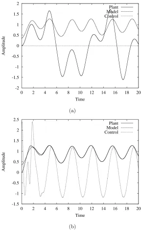
control can often be used successfully (Stoten & Di Bernardo, 1996). For example the problem discussed in Stoten & Di Bernardo (1996) is to synchronize the motion of two Duffing oscillators

¨

x+δx˙−σx+ǫx3

=qcos(ωt) +u(t) ¨

xm+δmx˙m−σmxm+ǫmx3m=qmcos(ωt). (32)

In this caseσm=σ= 1,δm=δ= 0.4 andǫm=ǫ= 1,ω = 1.8,q= 1.8

and qm= 0.62. As a result the error dynamics can be written as

˙ xe1

˙ xe2

=

0 1

σm −δm

xe1 xe2

+

0

−(x3

m−x

3

) + (qm−q) cos(ωt) +u(t)

(33) Here we have selected the parameter values such that the reference model has periodic behaviour when the initial conditions at the start of the simulation are xm(0) = 0.348751 and ˙xm(0) = 0.194153. The

plant has zero initial conditions, and a forcing amplitude which results in chaotic motion. In figure 3 (a) the controller is disabled, u(t) = 0, and the model and plant motions are quite different. In figure 3 (b) the controller is enabled and the two systems quickly synchronize.

We also note from equation (33) that as the two system synchronize x→xmthen the (x3m−x

3

) term tends to zero and the system becomes effectively linear in the steady state. Thus for this type of system, the linear adaptive controller only has to cope with nonlinear dynamics during the transient (or adaptive) stage.

4.2. Adaptive feedback linearization control

Dealing with generalised nonlinear adaptive control systems such as equation (31) is as yet an unsolved problem and an active area of research interest (Khalil, 1992), (Krsti´c, et al, 1995) (Sastry, 1999). A key approach to these types of systems is that of linearization (Sastry, 1999). In this work, we will consider the (scalar) case when g2 = 0 such that we can write

˙

xe(t) =−λxe+L−g1(u, t), (34) where L= ∆f +λxe, and λ > 0. This formulation is possible with a

wide variety of both linear and nonlinear systems (Di Benardo, 1996). It is clear from equation (34) that (L−g1(u, t)) → 0, and λ > 0 will stabilize the required equilibrium, xe = 0. Therefore if the

ex-plicit structure of f1 and f2 is known, L is the feedback linearization controller for the system. e.g.g1 =Landλ >0 givesxe →0 ast→ ∞.

-2 -1.5 -1 -0.5 0 0.5 1 1.5 2

0 2 4 6 8 10 12 14 16 18 20

Amplitude

Time

Plant Model Control

(a)

-1.5 -1 -0.5 0 0.5 1 1.5 2 2.5

0 2 4 6 8 10 12 14 16 18 20

Amplitude

Time

Plant Model Control

(b)

Figure 3. Numerical simulation of two Duffing systems being synchronized using MCS control. The reference signal is a sine wave with amplitude and frequency equal to 1. The controller parameters are α = 0.1, β = 0.01 and settling time

of constant parameters, and ξ represents the vector of system vari-ables. For such systems we can use an adaptive controller of the form g(u, t) =u=k(t)ξ, wherek(t) is the adaptive gain. This approach will give an adaptive feedback linearization controller for the system. Using these definitions equation (34) can be expressed as

˙

xe(t) =−λxe+φ(t)ξ(t), (35)

whereφ(t) =k∗_{−k(t) is the parameter error. We then need to find an}

expression for k(t) which stabilises the system such that φ(t) → 0 as t→ ∞. This we can achieve by choosing a trial Lyapunov function of the form

V(t) = x 2

e

2 + φT_φ

2ρ , (36)

whereρis the controller gain. Then the derivative ofV with respect to time is

˙

V(t) =xe(−λxe+φ(t)ξ(t)) +

1

ρφφ,˙ (37)

such that choosing ˙φ=−ρxeξ, results in ˙V =−λx2ewhich implies that

the controller is Lyapunov stable. Thus ˙φ = −k˙ = −ρxeξ, such that

the adaptive gain becomes

k=ρ

Z t

t=t0

xeξdt. (38)

Thus k(t) → k∗ _{as φ → 0 and xe → 0. We note also that providing}

φ → 0, the final adaptive gain values correspond to the unknown set of system parameters k∗_{. In general k(t)→ k}∗ _{providing the adaptive}

controller has a persistently exciting signal.

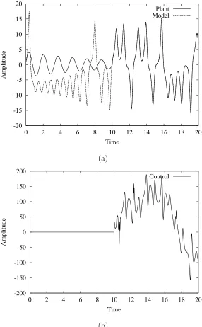
4.2.1. Example 3: Non-identical nonlinear systems

In this example we use a Chua system defined as

˙

x1 =α1(x2−x1) +α2x1−α3(|x1+ 1| − |x1−1|) ˙

x2 =x1−x2+x3 ˙

x3 =−δx2

(39)

and a Lorenz system

˙

y1=−σ(y1−y2) ˙

y2=Ry1−y2−y1y2 ˙

y3=y1y2−by3

(40)

for the system were selected as x1(0) = 1.1, x2(0) = 1.0, x3(0) = 7.0, y1(0) =−1.1,y2(0) =−1.0 and y1(0) =−5.0.

As our analysis is limited to control of scalar variables, we will consider the case when we wish to control x3 from the Chua system to follow y1 from the Lorenz system. To develop a controller we need to express L, the feedback linearization controller, as a product of an unknown parameter vector, k∗ _{and a system variable vector, ξ. Thus}

xe=y1−x3 and by takingλ=σ we obtain

L=σ(y2−x3) +δx2 ={σ, δ}

y2−x3 x2

(41)

so that the system variable vector is ξ = {(y2 −x3), x2}T and the parameter vector is k∗ _{= {σ, δ}, and as before the adaptive feedback}

linearization controller is u=k(t)ξ. In this example the control signal, u(t), is added to the expression for ˙x3

The response of the system is shown in figure 4, where the controller was initiated at timet= 10. In this figurex3 is referred to as the plant andy1 the model. The control parameters for this example wereρ= 50 and ts = 4.0. The control tracking after t = 10 is excellent, but the

control effort, as shown in figure 4 (b), is much larger than the linear adaptive control examples.

5. Conclusions

In this paper we have considered the application of model reference adaptive control techniques to nonlinear systems. In particular we have considered using the minimal control synthesis approach to model ref-erence adaptive control. This approach has been outlined in detail including a discussion on stability of such systems.

We have discussed how nonlinear systems with either small or identi-cal nonlinearity can often be controlled using a standard linear adaptive control, and a numerical example of each of these cases has been shown. For non-identical nonlinear systems we can take only a more limited approach, and we discussed how an adaptive feedback linearization controller could be developed. As an example we demonstrated how scalar variables from two different chaotic systems can be synchronized using this adaptive control approach.

-20 -15 -10 -5 0 5 10 15 20

0 2 4 6 8 10 12 14 16 18 20

Amplitude

Time

Plant Model

(a)

-200 -150 -100 -50 0 50 100 150 200

0 2 4 6 8 10 12 14 16 18 20

Amplitude

Time

Control

(b)

Acknowledgements

The author would like to thank Xiaofan Wang for helpful comments regarding this text.

References

Banks, S. P. (1986).Control systems engineering : modelling and simulation, control theory and microprocessor implementation. Englewood Cliffs : Prentice-Hall. Di Benardo, M. (1996). An adaptive approach to the control and synchronization

of continuous-time chaotic systems. International Journal of Bifurcation and Chaos 6(3), 557–568.

Goodwine, B. & St´ep´an, G. (2000). Controlling unstable rolling phenomena.Journal of Vibration and Control 6, 137–158.

Guckenheimer, J. & Holmes, P. (1983). Nonlinear oscillations, dynamical systems, and bifurcations of vector fields. New York: Springer-Verlag.

Khalil, H. K. (1992). Nonlinear Systems. Macmillan: New York.

Krsti´c, M., Kanellakopoulos, I. & Kokotovi´c, P. (1995). Nonlinear and adaptive control design. John Wiley.

Landau, Y. D. (1979). Adaptive control: The model reference approach. Marcel Dekker: New York.

Lin, Y-Y. & Lin, G-L. (2001). Non-linear control with Lyapunov stability applied to spacecraft with flexible structures. Proceedings of the I MECH E Part I: Journal of Systems and Control in Engineering 215(2), 131–141.

Menson, P. K. & Ohlmeyer, E. J. (2001). Integrated design of agile missile guidence and autopilot systems. Control Engineering Practice 9, 1095–1106.

Narendra, K. S. & Valavani, L. S. (1980). A comparison of lyapunov and hypersta-bility approaches to adaptive control of continuous systems. IEEE Transactions on automatic control 25(2), 243–247.

Ott, E., Grebogi, C. & Yorke, J. A. (1990). Controlling chaos. Physical Review Letters 64(11), 1196–1199.

Popov, V. M. (1973). Hyperstability of control systems. Springer.

Rao, M. P. R. V. (1998). Non-quadratic lyapunov function and adaptive laws for model reference adaptive control. Electronics Letters 34(23), 2278–2280. Sastry, S. (1999).Nonlinear systems: Analysis, stability and control. Springer-Verlag:

New York.

Sastry, S. & Bodson, M. (1989). Adaptive control: Stability, convergence and robustness. Prentice-Hall: New Jersey.

Stoten, D. P. (1993). An overview of the minimal control synthesis algorithm. In

I. Mech. E. Conference on Aerospace Hydraulics and Systems, London. Paper C474-033.

Stoten, D. P. & Benchoubane, H. (1990). Robustness of a minimal controller synthesis algorithm. International Journal of Control 51(4), 851–861.