Foundations of Cryptography
Cryptography is concerned with the conceptualization, definition, and construction of computing systems that address security concerns. The design of cryptographic systems must be based on firm foundations. This book presents a rigorous and systematic treatment of the foundational issues: defining cryptographic tasks and solving new cryptographic problems using existing tools. It focuses on the basic mathematical tools: computational difficulty (one-way functions), pseudorandomness, and zero-knowledge proofs. The emphasis is on the clarification of fundamental concepts and on demonstrat-ing the feasibility of solvdemonstrat-ing cryptographic problems rather than on describdemonstrat-ing ad hoc approaches.
Foundations of Cryptography
Basic Tools
Oded Goldreich
The Pitt Building, Trumpington Street, Cambridge, United Kingdom
The Edinburgh Building, Cambridge CB2 2RU, UK
40 West 20th Street, New York, NY 10011-4211, USA
477 Williamstown Road, Port Melbourne, VIC 3207, Australia
Ruiz de Alarcón 13, 28014 Madrid, Spain
Dock House, The Waterfront, Cape Town 8001, South Africa
http://www.cambridge.org
First published in printed format
ISBN 0-521-79172-3 hardback
ISBN 0-511-04120-9 eBook
Oded Goldreich 2004
First published 2001
Contents
List of Figures page xii
Preface xiii
1 Introduction 1
1.1. Cryptography: Main Topics 1
1.1.1. Encryption Schemes 2
1.1.2. Pseudorandom Generators 3
1.1.3. Digital Signatures 4
1.1.4. Fault-Tolerant Protocols and Zero-Knowledge Proofs 6
1.2. Some Background from Probability Theory 8
1.2.1. Notational Conventions 8
1.2.2. Three Inequalities 9
1.3. The Computational Model 12
1.3.1. P,N P, andN P-Completeness 12
1.3.2. Probabilistic Polynomial Time 13
1.3.3. Non-Uniform Polynomial Time 16
1.3.4. Intractability Assumptions 19
1.3.5. Oracle Machines 20
1.4. Motivation to the Rigorous Treatment 21
1.4.1. The Need for a Rigorous Treatment 21
1.4.2. Practical Consequences of the Rigorous Treatment 23
1.4.3. The Tendency to Be Conservative 24
1.5. Miscellaneous 25
1.5.1. Historical Notes 25
1.5.2. Suggestions for Further Reading 27
1.5.3. Open Problems 27
CONTENTS
2 Computational Difficulty 30
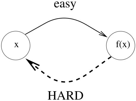
2.1. One-Way Functions: Motivation 31
2.2. One-Way Functions: Definitions 32
2.2.1. Strong One-Way Functions 32
2.2.2. Weak One-Way Functions 35
2.2.3. Two Useful Length Conventions 35
2.2.4. Candidates for One-Way Functions 40
2.2.5. Non-Uniformly One-Way Functions 41
2.3 Weak One-Way Functions Imply Strong Ones 43
2.3.1. The Construction and Its Analysis (Proof of Theorem 2.3.2) 44
2.3.2. Illustration by a Toy Example 48
2.3.3. Discussion 50
2.4. One-Way Functions: Variations 51
2.4.1.∗∗ Universal One-Way Function 52
2.4.2. One-Way Functions as Collections 53
2.4.3. Examples of One-Way Collections 55
2.4.4. Trapdoor One-Way Permutations 58
2.4.5.∗∗ Claw-Free Functions 60
2.4.6.∗∗ On Proposing Candidates 63
2.5. Hard-Core Predicates 64
2.5.1. Definition 64
2.5.2. Hard-Core Predicates for Any One-Way Function 65
2.5.3.∗∗ Hard-Core Functions 74
2.6.∗∗ Efficient Amplification of One-Way Functions 78
2.6.1. The Construction 80
2.6.2. Analysis 81
2.7. Miscellaneous 88
2.7.1. Historical Notes 89
2.7.2. Suggestions for Further Reading 89
2.7.3. Open Problems 91
2.7.4. Exercises 92
3 Pseudorandom Generators 101
3.1. Motivating Discussion 102
3.1.1. Computational Approaches to Randomness 102
3.1.2. A Rigorous Approach to Pseudorandom Generators 103
3.2. Computational Indistinguishability 103
3.2.1. Definition 104
3.2.2. Relation to Statistical Closeness 106
3.2.3. Indistinguishability by Repeated Experiments 107
3.2.4.∗∗ Indistinguishability by Circuits 111
3.2.5. Pseudorandom Ensembles 112
3.3. Definitions of Pseudorandom Generators 112
CONTENTS
3.3.2. Increasing the Expansion Factor 114
3.3.3.∗∗ Variable-Output Pseudorandom Generators 118
3.3.4. The Applicability of Pseudorandom Generators 119
3.3.5. Pseudorandomness and Unpredictability 119
3.3.6. Pseudorandom Generators Imply One-Way Functions 123
3.4. Constructions Based on One-Way Permutations 124
3.4.1. Construction Based on a Single Permutation 124
3.4.2. Construction Based on Collections of Permutations 131
3.4.3.∗∗ Using Hard-Core Functions Rather than Predicates 134
3.5.∗∗ Constructions Based on One-Way Functions 135
3.5.1. Using 1-1 One-Way Functions 135
3.5.2. Using Regular One-Way Functions 141
3.5.3. Going Beyond Regular One-Way Functions 147
3.6. Pseudorandom Functions 148
3.6.1. Definitions 148
3.6.2. Construction 150
3.6.3. Applications: A General Methodology 157
3.6.4.∗∗ Generalizations 158
3.7.∗∗ Pseudorandom Permutations 164
3.7.1. Definitions 164
3.7.2. Construction 166
3.8. Miscellaneous 169
3.8.1. Historical Notes 169
3.8.2. Suggestions for Further Reading 170
3.8.3. Open Problems 172
3.8.4. Exercises 172
4 Zero-Knowledge Proof Systems 184
4.1. Zero-Knowledge Proofs: Motivation 185
4.1.1. The Notion of a Proof 187
4.1.2. Gaining Knowledge 189
4.2. Interactive Proof Systems 190
4.2.1. Definition 190
4.2.2. An Example (Graph Non-Isomorphism inIP) 195
4.2.3.∗∗ The Structure of the ClassIP 198
4.2.4. Augmentation of the Model 199
4.3. Zero-Knowledge Proofs: Definitions 200
4.3.1. Perfect and Computational Zero-Knowledge 200
4.3.2. An Example (Graph Isomorphism inPZK) 207
4.3.3. Zero-Knowledge with Respect to Auxiliary Inputs 213
4.3.4. Sequential Composition of Zero-Knowledge Proofs 216
4.4. Zero-Knowledge Proofs forN P 223
4.4.1. Commitment Schemes 223
CONTENTS
4.4.3. The General Result and Some Applications 240
4.4.4. Second-Level Considerations 243
4.5.∗∗ Negative Results 246
4.5.1. On the Importance of Interaction and Randomness 247
4.5.2. Limitations of Unconditional Results 248
4.5.3. Limitations of Statistical ZK Proofs 250
4.5.4. Zero-Knowledge and Parallel Composition 251
4.6.∗∗ Witness Indistinguishability and Hiding 254
4.6.1. Definitions 254
4.6.2. Parallel Composition 258
4.6.3. Constructions 259
4.6.4. Applications 261
4.7.∗∗ Proofs of Knowledge 262
4.7.1. Definition 262
4.7.2. Reducing the Knowledge Error 267
4.7.3. Zero-Knowledge Proofs of Knowledge forN P 268
4.7.4. Applications 269
4.7.5. Proofs of Identity (Identification Schemes) 270
4.7.6. Strong Proofs of Knowledge 274
4.8.∗∗ Computationally Sound Proofs (Arguments) 277
4.8.1. Definition 277
4.8.2. Perfectly Hiding Commitment Schemes 278
4.8.3. Perfect Zero-Knowledge Arguments forN P 284
4.8.4. Arguments of Poly-Logarithmic Efficiency 286
4.9.∗∗ Constant-Round Zero-Knowledge Proofs 288
4.9.1. Using Commitment Schemes with Perfect Secrecy 289
4.9.2. Bounding the Power of Cheating Provers 294
4.10.∗∗ Non-Interactive Zero-Knowledge Proofs 298
4.10.1. Basic Definitions 299
4.10.2. Constructions 300
4.10.3. Extensions 306
4.11.∗∗ Multi-Prover Zero-Knowledge Proofs 311
4.11.1. Definitions 311
4.11.2. Two-Sender Commitment Schemes 313
4.11.3. Perfect Zero-Knowledge forN P 317
4.11.4. Applications 319
4.12. Miscellaneous 320
4.12.1. Historical Notes 320
4.12.2. Suggestions for Further Reading 322
4.12.3. Open Problems 323
4.12.4. Exercises 323
Appendix A: Background in Computational Number Theory 331
A.1. Prime Numbers 331
CONTENTS
A.1.2. Extracting Square Roots Modulo a Prime 332
A.1.3. Primality Testers 332
A.1.4. On Uniform Selection of Primes 333
A.2. Composite Numbers 334
A.2.1. Quadratic Residues Modulo a Composite 335
A.2.2. Extracting Square Roots Modulo a Composite 335
A.2.3. The Legendre and Jacobi Symbols 336
A.2.4. Blum Integers and Their Quadratic-Residue Structure 337
Appendix B: Brief Outline of Volume 2 338
B.1. Encryption: Brief Summary 338
B.1.1. Definitions 338
B.1.2. Constructions 340
B.1.3. Beyond Eavesdropping Security 343
B.1.4. Some Suggestions 345
B.2. Signatures: Brief Summary 345
B.2.1. Definitions 346
B.2.2. Constructions 347
B.2.3. Some Suggestions 349
B.3. Cryptographic Protocols: Brief Summary 350
B.3.1. Definitions 350
B.3.2. Constructions 352
B.3.3. Some Suggestions 353
Bibliography 355
Index 367
List of Figures
0.1 Organization of the work pagexvi
0.2 Rough organization of this volume xvii
0.3 Plan for one-semester course on the foundations of cryptography xviii
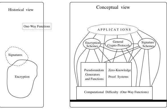
1.1 Cryptography: two points of view 25
2.1 One-way functions: an illustration 31
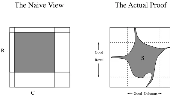
2.2 The naive view versus the actual proof of Proposition 2.3.3 49
2.3 The essence of Construction 2.6.3 81
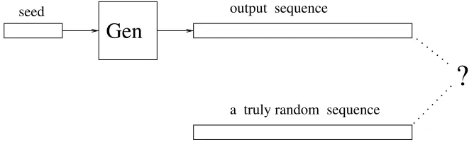
3.1 Pseudorandom generators: an illustration 102
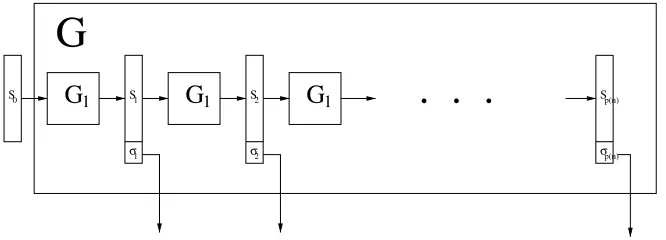
3.2 Construction 3.3.2, as operating on seeds0∈ {0, 1} n
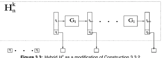
114 3.3 HybridHk
n as a modification of Construction 3.3.2 115 3.4 Construction 3.4.2, as operating on seeds0∈ {0, 1}
n
129
3.5 Construction 3.6.5, forn=3 151
3.6 The high-level structure of the DES 166
4.1 Zero-knowledge proofs: an illustration 185
4.2 The advanced sections of this chapter 185
4.3 The dependence structure of this chapter 186
Preface
It is possible to build a cabin with no foundations, but not a lasting building. Eng. Isidor Goldreich (1906–1995) Cryptography is concerned with the construction of schemes that should be able to withstand any abuse. Such schemes are constructed so as to maintain a desired func-tionality, even under malicious attempts aimed at making them deviate from their prescribed functionality.
The design of cryptographic schemes is a very difficult task. One cannot rely on intuitions regarding the typical state of the environment in which a system will operate. For sure, anadversaryattacking the system will try to manipulate the environment into untypical states. Nor can one be content with countermeasures designed to withstand specific attacks, because the adversary (who will act after the design of the system has been completed) will try to attack the schemes in ways that typically will be different from the ones the designer envisioned. Although the validity of the foregoing assertions seems self-evident, still some people hope that, in practice, ignoring these tautologies will not result in actual damage. Experience shows that such hopes are rarely met; cryp-tographic schemes based on make-believe are broken, typically sooner rather than later. In view of the foregoing, we believe that it makes little sense to make assumptions regarding the specificstrategythat an adversary may use. The only assumptions that can be justified refer to the computationalabilitiesof the adversary. Furthermore, it is our opinion that the design of cryptographic systems has to be based onfirm foundations, whereas ad hoc approaches and heuristics are a very dangerous way to go. A heuristic may make sense when the designer has a very good idea about the environment in which a scheme is to operate, but a cryptographic scheme will have to operate in a maliciously selected environment that typically will transcend the designer’s view.
PREFACE
obtained by using them. Our emphasis is on the clarification of fundamental concepts and on demonstrating the feasibility of solving several central cryptographic problems. Solving a cryptographic problem (or addressing a security concern) is a two-stage process consisting of adefinitional stageand aconstructive stage. First, in the defini-tional stage, the funcdefini-tionality underlying the natural concern must be identified and an adequate cryptographic problem must be defined. Trying to list all undesired situations is infeasible and prone to error. Instead, one should define the functionality in terms of operation in an imaginary ideal model and then require a candidate solution to emulate this operation in the real, clearly defined model (which will specify the adversary’s abilities). Once the definitional stage is completed, one proceeds to construct a system that will satisfy the definition. Such a construction may use some simpler tools, and its security is to be proved relying on the features of these tools. (In practice, of course, such a scheme also may need to satisfy some specific efficiency requirements.)
This book focuses on several archetypical cryptographic problems (e.g., encryption and signature schemes) and on several central tools (e.g., computational difficulty, pseu-dorandomness, and zero-knowledge proofs). For each of these problems (resp., tools), we start by presenting the natural concern underlying it (resp., its intuitive objective), then define the problem (resp., tool), and finally demonstrate that the problem can be solved (resp., the tool can be constructed). In the last step, our focus is on demonstrat-ing the feasibility of solvdemonstrat-ing the problem, not on providdemonstrat-ing a practical solution. As a secondary concern, we typically discuss the level of practicality (or impracticality) of the given (or known) solution.
Computational Difficulty
The specific constructs mentioned earlier (as well as most constructs in this area) can exist only if some sort of computational hardness (i.e., difficulty) exists. Specifically, all these problems and tools require (either explicitly or implicitly) the ability to gen-erate instances of hard problems. Such ability is captured in the definition of one-way functions (see further discussion in Section 2.1). Thus, one-way functions are the very minimum needed for doing most sorts of cryptography. As we shall see, they actually suffice for doing much of cryptography (and the rest can be done by augmentations and extensions of the assumption that one-way functions exist).
Our current state of understanding of efficient computation does not allow us to prove that one-way functions exist. In particular, the existence of one-way functions implies thatN P is not contained inBPP ⊇P (not even “on the average”), which would resolve the most famous open problem of computer science. Thus, we have no choice (at this stage of history) but to assume that one-way functions exist. As justification for this assumption we can only offer the combined beliefs of hundreds (or thousands) of researchers. Furthermore, these beliefs concern a simply stated assumption, and their validity is supported by several widely believed conjectures that are central to some fields (e.g., the conjecture that factoring integers is difficult is central to computational number theory).
PREFACE
to know what we want: As stated earlier, we must first clarify what exactly we do want; that is, we must go through the typically complex definitional stage. But once this stage is completed, can we just assume that the definition derived can be met? Not really: The mere fact that a definition has been derived doesnotmean that it can be met, and one can easily define objects that cannot exist (without this fact being obvious in the definition). The way to demonstrate that a definition is viable (and so the intuitive security concern can be satisfied at all) is to construct a solution based on abetter-understoodassumption (i.e., one that is more common and widely believed). For example, looking at the definition of zero-knowledge proofs, it is not a priori clear that such proofs exist at all (in a non-trivial sense). The non-triviality of the notion was first demonstrated by presenting a zero-knowledge proof system for statements regarding Quadratic Residuosity that are believed to be difficult to verify (without extra information). Furthermore, contrary to prior belief, it was later shown that the existence of one-way functions implies that anyN P-statement can be proved in zero-knowledge. Thus, facts that were not at all known to hold (and were even believed to be false) were shown to hold by reduction to widely believed assumptions (without which most of modern cryptography would collapse anyhow). To summarize, not all assumptions are equal, and so reducing a complex, new, and doubtful assumption to a widely believed simple (or even merely simpler) assumption is of great value. Furthermore, reducing the solution of a new task to the assumed security of a well-known primitive task typically means providing a construction that, using the known primitive, will solve the new task. This means that we not only know (or assume) that the new task is solvable but also have a solution based on a primitive that, being well known, typically has several candidate implementations.
Structure and Prerequisites
Our aim is to present the basic concepts, techniques, and results in cryptography. As stated earlier, our emphasis is on the clarification of fundamental concepts and the rela-tionships among them. This is done in a way independent of the particularities of some popular number-theoretic examples. These particular examples played a central role in the development of the field and still offer the most practical implementations of all cryptographic primitives, but this does not mean that the presentation has to be linked to them. On the contrary, we believe that concepts are best clarified when presented at an abstract level, decoupled from specific implementations. Thus, the most relevant background for this book is provided by basic knowledge of algorithms (including randomized ones), computability, and elementary probability theory. Background on (computational) number theory, which is required for specific implementations of cer-tain constructs, is not really required here (yet a short appendix presenting the most relevant facts is included in this volume so as to support the few examples of imple-mentations presented here).
PREFACE
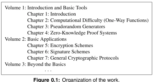
Volume 1: Introduction and Basic Tools Chapter 1: Introduction
Chapter 2: Computational Difficulty (One-Way Functions) Chapter 3: Pseudorandom Generators
Chapter 4: Zero-Knowledge Proof Systems Volume 2: Basic Applications
Chapter 5: Encryption Schemes Chapter 6: Signature Schemes
Chapter 7: General Cryptographic Protocols Volume 3: Beyond the Basics
[image:17.432.85.350.57.200.2]· · ·
Figure 0.1: Organization of the work.
(basic tools). It provides chapters on computational difficulty (one-way functions), pseudorandomness, and zero-knowledge proofs. These basic tools will be used for the basic applications in the second volume, which will consist of encryption, signatures, and general cryptographic protocols.
The partition of the work into three volumes is a logical one. Furthermore, it offers the advantage of publishing the first part without waiting for the completion of the other parts. Similarly, we hope to complete the second volume within a couple of years and publish it without waiting for the third volume.
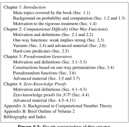
Organization of this first volume.This first volume consists of an introductory chap-ter (Chapchap-ter 1), followed by chapchap-ters on computational difficulty (one-way functions), pseudorandomness, and zero-knowledge proofs (Chapters 2–4, respectively). Also in-cluded are two appendixes, one of them providing a brief summary of Volume 2. Figure 0.2 depicts the high-level structure of this first volume.
Historical notes, suggestions for further reading, some open problems, and some exercises are provided at the end of each chapter. The exercises aremostlydesigned to assist and test one’s basic understanding of the main text, not to test or inspire creativity. The open problems are fairly well known; still, we recommend that one check their current status (e.g., at our updated-notices web site).
Web site for notices regarding this book.We intend to maintain a web site listing corrections of various types. The location of the site is
http://www.wisdom.weizmann.ac.il/∼oded/foc-book.html
Using This Book
PREFACE
Chapter 1:Introduction
Main topics covered by the book (Sec. 1.1)
Background on probability and computation (Sec. 1.2 and 1.3) Motivation to the rigorous treatment (Sec. 1.4)
Chapter 2:Computational Difficulty(One-Way Functions) Motivation and definitions (Sec. 2.1 and 2.2) One-way functions: weak implies strong (Sec. 2.3) Variants (Sec. 2.4) and advanced material (Sec. 2.6) Hard-core predicates (Sec. 2.5)
Chapter 3:Pseudorandom Generators Motivation and definitions (Sec. 3.1–3.3)
Constructions based on one-way permutations (Sec. 3.4) Pseudorandom functions (Sec. 3.6)
Advanced material (Sec. 3.5 and 3.7) Chapter 4:Zero-Knowledge Proofs
Motivation and definitions (Sec. 4.1–4.3) Zero-knowledge proofs forN P(Sec. 4.4) Advanced material (Sec. 4.5–4.11)
Appendix A: Background in Computational Number Theory Appendix B: Brief Outline of Volume 2
[image:18.432.87.345.56.310.2]Bibliography and Index
Figure 0.2:Rough organization of this volume.
only later pass to the technical details. The transition from high-level description to lower-level details is typically indicated by phrases such as “details follow.”
In a few places, we provide straightforward but tedious details in indented paragraphs such as this one. In some other (even fewer) places, such paragraphs provide technical proofs of claims that are of marginal relevance to the topic of the book.
More advanced material typically is presented at a faster pace and with fewer details. Thus, we hope that the attempt to satisfy a wide range of readers will not harm any of them.
Teaching.The material presented in this book is, on one hand, way beyond what one may want to cover in a semester course, and on the other hand it falls very short of what one may want to know about cryptography in general. To assist these conflicting needs, we make a distinction betweenbasicandadvancedmaterial and provide suggestions for further reading (in the last section of each chapter). In particular, those sections marked by an asterisk are intended for advanced reading.
PREFACE
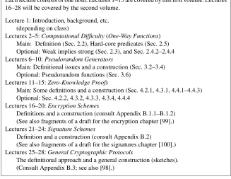
Each lecture consists of one hour. Lectures 1–15 are covered by this first volume. Lectures 16–28 will be covered by the second volume.
Lecture 1: Introduction, background, etc. (depending on class)
Lectures 2–5:Computational Difficulty(One-Way Functions) Main: Definition (Sec. 2.2), Hard-core predicates (Sec. 2.5) Optional: Weak implies strong (Sec. 2.3), and Sec. 2.4.2–2.4.4 Lectures 6–10:Pseudorandom Generators
Main: Definitional issues and a construction (Sec. 3.2–3.4) Optional: Pseudorandom functions (Sec. 3.6)
Lectures 11–15:Zero-Knowledge Proofs
Main: Some definitions and a construction (Sec. 4.2.1, 4.3.1, 4.4.1–4.4.3) Optional: Sec. 4.2.2, 4.3.2, 4.3.3, 4.3.4, 4.4.4
Lectures 16–20:Encryption Schemes
Definitions and a construction (consult Appendix B.1.1–B.1.2) (See also fragments of a draft for the encryption chapter [99].) Lectures 21–24:Signature Schemes
Definition and a construction (consult Appendix B.2)
(See also fragments of a draft for the signatures chapter [100].) Lectures 25–28:General Cryptographic Protocols
[image:19.432.53.380.71.324.2]The definitional approach and a general construction (sketches). (Consult Appendix B.3; see also [98].)
Figure 0.3:Plan for one-semester course on the foundations of cryptography.
we suggest the use of other sources for the second half. A brief summary of Volume 2 and recommendations for alternative sources are given in Appendix B. (In addition, fragments and/or preliminary drafts for the three chapters of Volume 2 are available from earlier texts, [99], [100], and [98], respectively.)
A course based solely on the material in this first volume is indeed possible, but such a course cannot be considered a stand-alone course in cryptography because this volume does not consider at all the basic tasks of encryption and signatures.
Practice.The aim of this work is to provide sound theoretical foundations for cryp-tography. As argued earlier, such foundations are necessary for any sound practice of cryptography. Indeed, sound practice requires more than theoretical foundations, whereas this work makes no attempt to provide anything beyond the latter. However, given sound foundations, one can learn and evaluate various practical suggestions that appear elsewhere (e.g., [158]). On the other hand, the absence of sound foundations will result in inability to critically evaluate practical suggestions, which in turn will lead to unsound decisions. Nothing could be more harmful to the design of schemes that need to withstand adversarial attacks than misconceptions about such attacks.
PREFACE
summary of this work. The other two chapters ofModern Cryptography,Probabilistic Proofs and Pseudorandomness[97] provide a wider perspective on two topics men-tioned in this volume (i.e., probabilistic proofs and pseudorandomness). Further com-ments on the latter aspect are provided in the relevant chapters of this volume.
Acknowledgments
First of all, I would like to thank three remarkable people who had a tremendous influence on my professional development: Shimon Even introduced me to theoretical computer science and closely guided my first steps. Silvio Micali and Shafi Goldwasser led my way in the evolving foundations of cryptography and shared with me their ongoing efforts toward further development of those foundations.
I have collaborated with many researchers, but I feel that my work with Benny Chor and Avi Wigderson has had the most important impact on my professional development and career. I would like to thank them both for their indispensable contributions to our joint research and for the excitement and pleasure of working with them.
Leonid Levin deserves special thanks as well. I have had many interesting discussions with Leonid over the years, and sometimes it has taken me too long to realize how helpful those discussions have been.
Next, I would like to thank a few colleagues and friends with whom I have had significant interactions regarding cryptography and related topics. These include Noga Alon, Boaz Barak, Mihir Bellare, Ran Canetti, Ivan Damgard, Uri Feige, Shai Halevi, Johan Hastad, Amir Herzberg, Russell Impagliazzo, Joe Kilian, Hugo Krawcyzk, Eyal Kushilevitz, Yehuda Lindell, Mike Luby, Daniele Micciancio, Moni Naor, Noam Nisan, Andrew Odlyzko, Yair Oren, Rafail Ostrovsky, Erez Petrank, Birgit Pfitzmann, Omer Reingold, Ron Rivest, Amit Sahai, Claus Schnorr, Adi Shamir, Victor Shoup, Madhu Sudan, Luca Trevisan, Salil Vadhan, Ronen Vainish, Yacob Yacobi, and David Zuckerman.
Even assuming I have not overlooked people with whom I have had significant interactions on topics related to this book, the complete list of people to whom I am indebted is far more extensive. It certainly includes the authors of many papers mentioned in the Bibliography. It also includes the authors of many cryptography-related papers that I have not cited and the authors of many papers regarding the theory of computation at large (a theory taken for granted in this book).
C H A P T E R
1
Introduction
In this chapter we briefly discuss the goals of cryptography (Section 1.1). In particular, we discuss the basic problems of secure encryption, digital signatures, and fault-tolerant protocols. These problems lead to the notions of pseudorandom generators and zero-knowledge proofs, which are discussed as well.
Our approach to cryptography is based on computational complexity. Hence, this introductory chapter also contains a section presenting the computational models used throughout the book (Section 1.3). Likewise, this chapter contains a section presenting some elementary background from probability theory that is used extensively in the book (Section 1.2).
Finally, we motivate the rigorous approach employed throughout this book and discuss some of its aspects (Section 1.4).
Teaching Tip.Parts of Section 1.4 may be more suitable for the last lecture (i.e., as part of the concluding remarks) than for the first one (i.e., as part of the introductory remarks). This refers specifically to Sections 1.4.2 and 1.4.3.
1.1. Cryptography: Main Topics
INTRODUCTION
We start by mentioning that much of the content of this book relies on the assump-tion that one-way funcassump-tions exist. The definiassump-tion of one-way funcassump-tions captures the sort of computational difficulty that is inherent to our entire approach to cryptography, an approach that attempts to capitalize on the computational limitations of any real-life adversary. Thus, if nothing is difficult, then this approach fails. However, if, as is widely believed, not only do hard problems exist but also instances of them can be efficiently generated, then these hard problems can be “put to work.” Thus, “algorithmically bad news” (by which hard computational problems exist) implies good news for cryptogra-phy. Chapter 2 is devoted to the definition and manipulation of computational difficulty in the form of one-way functions.
1.1.1. Encryption Schemes
The problem of providingsecret communication over insecure mediais the most tra-ditional and basic problem of cryptography. The setting consists of two parties com-municating over a channel that possibly may be tapped by an adversary, called the wire-tapper. The parties wish to exchange information with each other, but keep the wire-tapper as ignorant as possible regarding the content of this information. Loosely speaking, an encryption scheme is a protocol allowing these parties to communicate se-cretlywith each other. Typically, the encryption scheme consists of a pair of algorithms. One algorithm, calledencryption, is applied by the sender (i.e., the party sending a mes-sage), while the other algorithm, calleddecryption, is applied by the receiver. Hence, in order to send a message, the sender first applies the encryption algorithm to the message and sends the result, called theciphertext, over the channel. Upon receiving a ciphertext, the other party (i.e., the receiver) applies the decryption algorithm to it and retrieves the original message (called theplaintext).
In order for this scheme to provide secret communication, the communicating parties (at least the receiver) must know something that is not known to the wire-tapper. (Other-wise, the wire-tapper could decrypt the ciphertext exactly as done by the receiver.) This extra knowledge may take the form of the decryption algorithm itself or some parameters and/or auxiliary inputs used by the decryption algorithm. We call this extra knowledge thedecryption key. Note that, without loss of generality, we can assume that the decryp-tion algorithm is known to the wire-tapper and that the decrypdecryp-tion algorithm needs two inputs: a ciphertext and a decryption key. We stress that the existence of a secret key, not known to the wire-tapper, is merely a necessary condition for secret communication.
1.1. CRYPTOGRAPHY: MAIN TOPICS
schemes. This is especially true whenhugeamounts of information need to be secretly communicated.
The second (“modern”) approach, as followed in this book, is based oncomputational complexity. This approach is based on the fact thatit does not matter whether or not the ciphertext contains information about the plaintext, but ratherwhether or not this information can be efficiently extracted. In other words, instead of asking whether or not it ispossiblefor the wire-tapper to extract specific information, we ask whether or not it isfeasiblefor the wire-tapper to extract this information. It turns out that the new (i.e., “computational-complexity”) approach offers security even if the key is much shorter than the total length of the messages sent via the encryption scheme. For example, one can use “pseudorandom generators” (discussed later) that expand short keys into much longer “pseudo-keys,” so that the latter are as secure as “real keys” of comparable length. In addition, the computational-complexity approach allows the introduction of con-cepts and primitives that cannot exist under the information-theoretic approach. A typical example is the concept ofpublic-key encryption schemes. Note that in the pre-ceding discussion we concentrated on the decryption algorithm and its key. It can be shown that the encryption algorithm must get, in addition to the message, an auxiliary input that depends on the decryption key. This auxiliary input is called the encryp-tion key. Traditional encryption schemes, and in particular all the encryption schemes used over the millennia preceding the 1980s, operate with an encryption key equal to the decryption key. Hence, the wire-tapper in these schemes must be ignorant of the encryption key, and consequently the key-distribution problem arises (i.e., how two parties wishing to communicate over an insecure channel can agree on a secret encryption/decryption key).1The computational-complexity approach allows the
in-troduction of encryption schemes in which the encryption key can be known to the wire-tapper without compromising the security of the scheme. Clearly, the decryption key in such schemes is different from the encryption key, and furthermore it is infeasi-ble to compute the decryption key from the encryption key. Such encryption schemes, calledpublic-key schemes, have the advantage of trivially resolving the key-distribution problem, because the encryption key can be publicized.
In Chapter 5, which will appear in the second volume of this work and will be devoted to encryption schemes, we shall discuss private-key and public-key encryption schemes. Much attention is devoted to defining the security of encryption schemes. Finally, con-structions of secure encryption schemes based on various intractability assumptions are presented. Some of the constructions presented are based on pseudorandom generators, which are discussed in Chapter 3. Other constructions use specific one-way functions such as the RSA function and/or the operation of squaring modulo a composite number.
1.1.2. Pseudorandom Generators
It turns out that pseudorandom generators play a central role in the construction of encryption schemes (and related schemes). In particular, pseudorandom generators
1The traditional solution is to exchange the key through an alternative channel that is secure, alas “more
INTRODUCTION
yield simple constructions of private-key encryption schemes, and this observation is often used in practice (usually implicitly).
Although the term “pseudorandom generators” is commonly usedin practice, both in the context of cryptography and in the much wider context of probabilistic procedures, it is seldom associated with a precise meaning. We believe that using a term without clearly stating what it means is dangerous in general and particularly so in a tricky business such as cryptography. Hence, a precise treatment of pseudorandom generators is central to cryptography.
Loosely speaking, a pseudorandom generator is a deterministic algorithm that ex-pands short random seeds into much longer bit sequences thatappearto be “random” (although they are not). In other words, although the output of a pseudorandom generator is not really random, it isinfeasibleto tell the difference. It turns out that pseudoran-domness and computational difficulty are linked in an even more fundamental manner, as pseudorandom generators can be constructed based on various intractability assump-tions. Furthermore, the main result in this area asserts that pseudorandom generators exist if and only if one-way functions exist.
Chapter 3, devoted to pseudorandom generators, starts with a treatment of the con-cept of computational indistinguishability. Pseudorandom generators are defined next and are constructed using special types of one-way functions (defined in Chapter 2). Pseudorandomfunctionsare defined and constructed as well. The latter offer a host of additional applications.
1.1.3. Digital Signatures
A notion that did not exist in the pre-computerized world is that of a “digital signature.” The need to discuss digital signatures arose with the introduction of computer commu-nication in the business environment in which parties need to commit themselves to proposals and/or declarations they make. Discussions of “unforgeable signatures” also took place in previous centuries, but the objects of discussion were handwritten signa-tures, not digital ones, and the discussion was not perceived as related to cryptography. Relations between encryption and signature methods became possible with the “digitalization” of both and the introduction of the computational-complexity approach to security. Loosely speaking, ascheme for unforgeable signaturesrequires
• that each user be ableto efficiently generate his or her own signatureon documents of his or her choice,
• that each user be ableto efficiently verifywhether or not a given string is a signature of another (specific) user on a specific document, and
• thatno one be able to efficiently produce the signatures of other usersto documents that those users did not sign.
1.1. CRYPTOGRAPHY: MAIN TOPICS
difficult) to forge signatures in a manner that could pass the verification procedure. It is difficult to state to what extent handwritten signatures meet these requirements. In contrast, our discussion of digital signatures will supply precise statements concern-ing the extent to which digital signatures meet the foregoconcern-ing requirements. Further-more, schemes for unforgeable digital signatures can be constructed using the same computational assumptions as used in the construction of (private-key) encryption schemes.
In Chapter 6, which will appear in the second volume of this work and will be devoted to signature schemes, much attention will be focused on defining the security (i.e., unforgeability) of these schemes. Next, constructions of unforgeable signature schemes based on various intractability assumptions will be presented. In addition, we shall treat the related problem of message authentication.
Message Authentication
Message authentication is a task related to the setting considered for encryption schemes (i.e., communication over an insecure channel). This time, we consider the case of an active adversary who is monitoring the channel and may alter the messages sent on it. The parties communicating through this insecure channel wish to authenticate the messages they send so that the intended recipient can tell an original message (sent by the sender) from a modified one (i.e., modified by the adversary). Loosely speaking, a scheme for message authenticationrequires
• that each of the communicating parties be ableto efficiently generate an authentication tagfor any message of his or her choice,
• that each of the communicating parties be ableto efficiently verifywhether or not a given string is an authentication tag for a given message, and
• thatno external adversary(i.e., a party other than the communicating parties)be able to efficiently produce authentication tags to messages not sent by the communicating parties.
In some sense, “message authentication” is similar to a digital signature. The difference between the two is that in the setting of message authentication it is not required that third parties (who may be dishonest) be able to verify the validity of authentication tags produced by the designated users, whereas in the setting of signature schemes it is required that such third parties be able to verify the validity of signatures produced by other users. Hence, digital signatures provide a solution to the message-authentication problem. On the other hand, a message-authentication scheme does not necessarily constitute a digital-signature scheme.
Signatures Widen the Scope of Cryptography
INTRODUCTION
• In the secret-communication problem (solved by use of encryption schemes), one wishes to reduce, as much as possible, the information that a potential wire-tapper can extract from the communication between two designated users. In this case, the designated system consists of the two communicating parties, and the wire-tapper is considered as an external (“dishonest”) party.
• In the message-authentication problem, one aims at prohibiting any (external) wire-tapper from modifying the communication between two (designated) users.
• In the signature problem, one aims at providing all users of a system a way of making self-binding statements and of ensuring that one user cannot make statements that would bind another user. In this case, the designated system consists of the set of all users, and a potential forger is considered as an internal yet dishonest user.
Hence, in the wide sense,cryptography is concerned with any problem in which one wishes to limit the effects of dishonest users. A general treatment of such problems is captured by the treatment of “fault-tolerant” (or cryptographic) protocols.
1.1.4. Fault-Tolerant Protocols and Zero-Knowledge Proofs
A discussion of signature schemes naturally leads to a discussion of cryptographic pro-tocols, because it is a natural concern to ask under what circumstances one party should provide its signature to another party. In particular, problems like mutual simultaneous commitment (e.g., contract signing) arise naturally. Another type of problem, motivated by the use of computer communication in the business environment, consists of “secure implementation” of protocols (e.g., implementing secret and incorruptible voting). Simultaneity Problems
A typical example of a simultaneity problem is that of simultaneous exchange of secrets, of which contract signing is a special case. The setting for a simultaneous exchange of secrets consists of two parties, each holding a “secret.” The goal is to execute a protocol such that if both parties follow it correctly, then at termination each will hold its counterpart’s secret, and in any case (even if one party cheats) the first party will hold the second party’s secret if and only if the second party holds the first party’s secret. Perfectly simultaneous exchange of secrets can be achieved only if we assume the existence of third parties that are trusted to some extent. In fact, simultaneous exchange of secrets can easily be achieved using the active participation of a trusted third party: Each party sends its secret to the trusted third party (using a secure channel). The third party, on receiving both secrets, sends the first party’s secret to the second party and the second party’s secret to the first party. There are two problems with this solution:
1. The solution requires theactiveparticipation of an “external” party in all cases (i.e., also in case both parties are honest). We note that other solutions requiring milder forms of participation of external parties do exist.
1.1. CRYPTOGRAPHY: MAIN TOPICS
of implementing a trusted third party by a set of users with an honest majority (even if the identity of the honest users is not known).
Secure Implementation of Functionalities and Trusted Parties
A different type of protocol problem is concerned with the secure implementation of functionalities. To be more specific, we discuss the problem of evaluating a func-tion of local inputs each of which is held by a different user. An illustrative and motivating example isvoting, in which the function is majority, and the local input held by user Ais a single bit representing the vote of user A(e.g., “pro” or “con”). Loosely speaking, a protocol for securely evaluating a specific function must satisfy the following:
• Privacy: No party can “gain information” on the input of other parties, beyond what is deduced from the value of the function.
• Robustness: No party can “influence” the value of the function, beyond the influence exerted by selecting its own input.
It is sometimes required that these conditions hold with respect to “small” (e.g., minor-ity) coalitions of parties (instead of single parties).
Clearly, if one of the users is known to be totally trustworthy, then there exists a simple solution to the problem of secure evaluation of any function. Each user simply sends its input to the trusted party (using a secure channel), who, upon receiving all inputs, computes the function, sends the outcome to all users, and erases all interme-diate computations (including the inputs received) from its memory. Certainly, it is unrealistic to assume that a party can be trusted to such an extent (e.g., that it will voluntarily erase what it has “learned”). Nevertheless, the problem of implementing secure function evaluation reduces to the problem of implementing a trusted party. It turns out that a trusted party can be implemented by a set of users with an hon-est majority (even if the identity of the honhon-est users is not known). This is indeed a major result in this field, and much of Chapter 7, which will appear in the second volume of this work, will be devoted to formulating and proving it (as well as variants of it).
Zero-Knowledge as a Paradigm
A major tool in the construction of cryptographic protocols is the concept of zero-knowledgeproof systems and the fact that zero-knowledge proof systems exist for all languages inN P (provided that one-way functions exist). Loosely speaking, a zero-knowledge proof yields nothing but the validity of the assertion. Zero-zero-knowledge proofs provide a tool for “forcing” parties to follow a given protocol properly.
INTRODUCTION
required. A much better idea is to let Alice augment the bit she sends Carol with a zero-knowledge proof that this bit is indeed the least significant bit of the message. We stress that the foregoing statement is of the “N Ptype” (since the proof specified earlier can be efficiently verified), and therefore the existence of zero-knowledge proofs for N P-statements implies that the foregoing statement can be proved without revealing anything beyond its validity.
The focus of Chapter 4, devoted to zero-knowledge proofs, is on the foregoing result (i.e., the construction of zero-knowledge proofs for anyN P-statement). In addition, we shall consider numerous variants and aspects of the notion of zero-knowledge proofs and their effects on the applicability of this notion.
1.2. Some Background from Probability Theory
Probability plays a central role in cryptography. In particular, probability is essential in order to allow a discussion of information or lack of information (i.e., secrecy). We assume that the reader is familiar with the basic notions of probability theory. In this section, we merely present the probabilistic notations that are used throughout this book and three useful probabilistic inequalities.
1.2.1. Notational Conventions
Throughout this entire book we shall refer to onlydiscreteprobability distributions. Typically, the probability space consists of the set of all strings of a certain length , taken with uniform probability distribution. That is, the sample space is the set of all -bit-long strings, and each such string is assigned probability measure 2−. Traditionally, functions from the sample space to the reals are calledrandom variables. Abusing standard terminology, we allow ourselves to use the termrandom variablealso when referring to functions mapping the sample space into the set of binary strings. We often do not specify the probability space, but rather talk directly about random variables. For example, we may say that X is a random variable assigned values in the set of all strings, so thatPr[X =00]= 14 andPr[X =111]= 34. (Such a random variable can be defined over the sample space{0,1}2, so thatX(11)=00 andX(00)=
X(01)= X(10)=111.) In most cases the probability space consists of all strings of a particular length. Typically, these strings represent random choices made by some randomized process (see next section), and the random variable is the output of the process.
How to Read Probabilistic Statements.All our probabilistic statements refer to functions of random variables that are defined beforehand. Typically, we shall write
1.2. SOME BACKGROUND FROM PROBABILITY THEORY
Namely,
Pr[B(X,X)]=
x
Pr[X =x]·χ(B(x,x))
whereχis an indicator function, so thatχ(B)=1 if eventBholds, and equals zero oth-erwise. For example, for every random variableX, we havePr[X= X]=1. We stress that if one wishes to discuss the probability thatB(x,y) holds whenxandyare chosen independently with the same probability distribution, then one needs to definetwo inde-pendent random variables, both with the same probability distribution. Hence, ifXand Yare two independent random variables, thenPr[B(X,Y)] denotes the probability that B(x,y) holds when the pair (x,y) is chosen with probabilityPr[X =x]·Pr[Y =y]. Namely,
Pr[B(X,Y)]=
x,y
Pr[X =x]·Pr[Y =y]·χ(B(x,y))
For example, for every two independent random variables, X and Y, we have
Pr[X=Y]=1 only if both X and Y are trivial (i.e., assign the entire probability mass to a single string).
Typical Random Variables.Throughout this entire book,Undenotes a random
vari-able uniformly distributed over the set of strings of lengthn. Namely,Pr[Un =α] equals
2−n ifα∈ {0,1}n, and equals zero otherwise. In addition, we shall occasionally use
random variables (arbitrarily) distributed over{0,1}n or{0,1}l(n)for some functionl:
N→N. Such random variables are typically denoted byXn,Yn,Zn, etc. We stress that in
some casesXnis distributed over{0,1}n, whereas in others it is distributed over{0,1}l(n),
for some functionl(·), which is typically a polynomial. Another type of random variable, the output of a randomized algorithm on a fixed input, is discussed in Section 1.3.
1.2.2. Three Inequalities
The following probabilistic inequalities will be very useful in the course of this book. All inequalities refer to random variables that are assigned real values. The most ba-sic inequality is theMarkov inequality, which asserts that for random variables with bounded maximum or minimum values, some relation must exist between the devia-tion of a value from the expectadevia-tion of the random variable and the probability that the random variable is assigned this value. Specifically, lettingE(X)def=vPr[X=v]·v denote the expectation of the random variableX, we have the following:
Markov Inequality: Let X be a non-negative random variable andv a real number. Then
Pr[X≥v]≤ E(X) v
INTRODUCTION
Proof:
E(X)=
x
Pr[X= x]·x
≥
x<v
Pr[X= x]·0+
x≥v
Pr[X =x]·v =Pr[X≥v]·v
The claim follows.
The Markov inequality is typically used in cases in which one knows very little about the distribution of the random variable; it suffices to know its expectation and at least one bound on the range of its values. See Exercise 1.
Using Markov’s inequality, one gets a “possibly stronger” bound for the deviation of a random variable from its expectation. This bound, called Chebyshev’s inequal-ity, is useful provided one has additional knowledge concerning the random variable (specifically, a good upper bound on its variance). For a random variable X of finite expectation, we denote byVar(X)def=E[(X−E(X))2] the variance ofX and observe
thatVar(X)=E(X2)−E(X)2.
Chebyshev’s Inequality:Let X be a random variable, andδ >0. Then
Pr[|X−E(X)| ≥δ]≤ Var(X) δ2
Proof: We define a random variable Y def= (X−E(X))2 and apply the Markov
inequality. We get
Pr[|X−E(X)| ≥δ]=Pr[(X−E(X))2 ≥δ2] ≤ E[(X−E(X))2]
δ2
and the claim follows.
Chebyshev’s inequality is particularly useful for analysis of the error probability of approximation via repeated sampling. It suffices to assume that the samples are picked in a pairwise-independent manner.
Corollary (Pairwise-Independent Sampling):Let X1,X2, . . . ,Xnbe pairwise-independent random variables with the same expectation, denotedµ, and the same variance, denotedσ2. Then, for everyε >0,
Pr
n
i=1Xi
n −µ
≥ε
≤ σ2 ε2n
The Xi’s are calledpairwise-independentif for everyi = j and allaandb, it holds
1.2. SOME BACKGROUND FROM PROBABILITY THEORY
Proof: Define the random variables Xi def
= Xi−E(Xi). Note that the Xi’s are
pairwise-independent and each has zero expectation. Applying Chebyshev’s in-equality to the random variable defined by the sumni=1 Xi
n , and using the linearity
of the expectation operator, we get
Pr
n
i=1 Xi
n −µ
≥ε ≤ Var n i=1 Xi n ε2 = E n
i=1Xi 2
ε2·n2
Now (again using the linearity ofE)
E n i=1 Xi 2
=n
i=1
EX2i +
1≤i=j≤n
E[XiXj]
By the pairwise independence of theXi’s, we getE[XiXj]=E[Xi]·E[Xj], and
usingE[Xi]=0, we get
E
n
i=1
Xi 2
=n·σ2
The corollary follows.
Using pairwise-independent sampling, the error probability in the approximation is decreasing linearly with the number of sample points. Using totally independent sampling points, the error probability in the approximation can be shown to decrease exponentially with the number of sample points. (The random variablesX1,X2, . . . ,Xn
are said to be totally independentif for every sequence a1,a2, . . . ,an it holds that
Pr[∧n
i=1Xi =ai] equals
n
i=1Pr[Xi =ai].) Probability bounds supporting the
forego-ing statement are given next. The first bound, commonly referred to as the Chernoff bound, concerns 0-1 random variables (i.e., random variables that are assigned values of either 0 or 1).
Chernoff Bound: Let p≤ 1
2, and let X1,X2, . . . ,Xnbe independent0-1random
variables, so thatPr[Xi =1]= p for each i . Then for allε,0< ε≤ p(1− p), we have
Pr
n
i=1Xi
n −p
> ε
<2·e− ε 2 2p(1−p)·n
We shall usually apply the bound with a constant p≈ 12. In this case,nindependent samples give an approximation that deviates byεfrom the expectation with probabilityδ that is exponentially decreasing withε2n. Such an approximation is called an (ε, δ)
INTRODUCTION
error probability (i.e.,δ) can be made negligible (as a function inn), but the accuracy of the estimation (i.e.,ε) can be bounded above only by any fixed polynomial fraction (but cannot be made negligible).2We stress that the dependence of the number of samples
onεis not better than in the case of pairwise-independent sampling; the advantage of totally independent samples lies only in the dependence of the number of samples onδ. A more general bound, useful for approximation of the expectation of a general random variable (not necessarily 0-1), is given as follows:
Hoefding Inequality:3Let X
1,X2, . . . ,Xn be n independent random variables with the same probability distribution, each ranging over the (real) interval[a,b], and letµdenote the expected value of each of these variables. Then, for every ε >0,
Pr
n
i=1Xi
n −µ
> ε
<2·e− 2ε 2 (b−a)2·n
The Hoefding inequality is useful for estimating the average value of a function defined over a large set of values, especially when the desired error probability needs to be negligible. It can be applied provided we can efficiently sample the set and have a bound on the possible values (of the function). See Exercise 2.
1.3. The Computational Model
Our approach to cryptography is heavily based on computational complexity. Thus, some background on computational complexity is required for our discussion of cryp-tography. In this section, we briefly recall the definitions of the complexity classesP, N P,BPP, and “non-uniformP” (i.e.,P/poly) and the concept of oracle machines. In addition, we discuss the types of intractability assumptions used throughout the rest of this book.
1.3.1.
P
,NP
, andNP
-CompletenessA conservative approach to computing devices associates efficient computations with the complexity classP. Jumping ahead, we note that the approach taken in this book is a more liberal one in that it allows the computing devices to be randomized.
Definition 1.3.1 (Complexity ClassPP): A language L isrecognizable in (deter-ministic)polynomial timeif there exists a deterministic Turing machine M and a polynomial p(·)such that
r
on input a string x, machine M halts after at most p(|x|)steps, andr
M(x)=1if and only if x ∈L.2Here and in the rest of this book, we denote by poly() some fixed but unspecified polynomial. 3A more general form requires the X
i’s to be independent, but not necessarily identical, and uses µdef
= 1
n
n
1.3. THE COMPUTATIONAL MODEL
P is the class of languages that can be recognized in (deterministic) polynomial time.
Likewise, the complexity classN Pis associated with computational problems having solutions that, once given, can be efficiently tested for validity. It is customary to define N P as the class of languages that can be recognized by a non-deterministic polynomial-time Turing machine. A more fundamental formulation ofN Pis given by the following equivalent definition.
Definition 1.3.2 (Complexity ClassN PN PN P): A language L is inN Pif there exists a Boolean relation RL ⊆ {0,1}∗× {0,1}∗and a polynomial p(·)such that RLcan be recognized in (deterministic) polynomial time, and x ∈L if and only if there exists a y such that|y| ≤ p(|x|)and(x,y)∈RL. Such a y is called awitness
for membershipof x ∈L.
Thus,N Pconsists of the set of languages for which there exist short proofs of member-ship that can be efficiently verified. It is widely believed thatP =N P, and resolution of this issue is certainly the most intriguing open problem in computer science. If indeed P =N P, then there exists a languageL∈N Psuch that every algorithm recognizing L will have a super-polynomial running time in the worst case. Certainly, allN P -complete languages (defined next) will have super-polynomial-time complexityin the worst case.
Definition 1.3.3 (N PN PN P-Completeness):A language isN P-completeif it is in
N P and every language inN P is polynomially reducible to it. A language L is polynomially reducibleto a language L if there exists a polynomial-time-computable function f such that x ∈L if and only if f(x)∈L.
Among the languages known to beN P-complete areSatisfiability(of propositional formulae),Graph Colorability, andGraph Hamiltonicity.
1.3.2. Probabilistic Polynomial Time
Randomized algorithms play a central role in cryptography. They are needed in or-der to allow the legitimate parties to generate secrets and are therefore allowed also to the adversaries. The reader is assumed to be familiar and comfortable with such algorithms.
1.3.2.1. Randomized Algorithms: An Example
INTRODUCTION
Testing whether or not a graph is connected is easily reduced to testing connectivity between any given pair of vertices.4Thus, we focus on the task of determining whether
or not two given vertices are connected in a given graph.
Algorithm.On input a graphG =(V,E) and two vertices,sandt, we take arandom walkof length O(|V| · |E|), starting at vertexs, and test at each step whether or not vertextis encountered. If vertext is ever encountered, then the algorithm will accept; otherwise, it will reject. By a random walk we mean that at each step we uniformly select one of the edges incident at the current vertex and traverse this edge to the other endpoint.
Analysis.Clearly, ifsis not connected totin the graphG, then the probability that the foregoing algorithm will accept will be zero. The harder part of the analysis is to prove that ifsis connected totin the graphG, then the algorithm will accept with probability at least 23. (The proof is deferred to Exercise 3.) Thus, either way, the algorithm will err with probability at most 13. The error probability can be further reduced by invoking the algorithm several times (using fresh random choices in each try).
1.3.2.2. Randomized Algorithms: Two Points of View
Randomized algorithms (machines) can be viewed in two equivalent ways. One way of viewing randomized algorithms is to allow the algorithm to make random moves (i.e., “toss coins”). Formally, this can be modeled by a Turing machine in which the transition function maps pairs of the form (state,symbol) to two possible triples of the form (state,symbol,direction). The next step for such a machine is determined by a random choice of one of these triples. Namely, to make a step, the machine chooses at random (with probability 12for each possibility) either the first triple or the second one and then acts accordingly. These random choices are called theinternal coin tossesof the machine. The output of a probabilistic machine M on input x is not a string but rather a random variable that assumes strings as possible values. This random variable, denotedM(x), is induced by the internal coin tosses ofM. ByPr[M(x)= y] we mean the probability that machineM on inputxwill outputy. The probability space is that of all possible outcomes for the internal coin tosses taken with uniform probability distribution.5 Because we consider only polynomial-time machines, we can assume,
without loss of generality, that the number of coin tosses made by M on input x is independent of their outcome and is denoted bytM(x). We denote byMr(x) the output
ofMon inputxwhenris the outcome of its internal coin tosses. ThenPr[M(x)=y]
4The space complexity of such a reduction is low; we merely need to store the names of two vertices (currently
being tested). Alas, the time complexity is indeed relatively high; we need to invoke the two-vertex testern2 times, wherenis the number of vertices in the graph.
5This sentence is slightly more problematic than it seems. The simple case is when, on inputx, machineM
always makes the same number of internal coin tosses (independent of their outcome). In general, the number of coin tosses may depend on the outcome of prior coin tosses. Still, for everyr, the probability that the outcome of the sequence of internal coin tosses will berequals 2−|r|if the machine does not terminate when the sequence
1.3. THE COMPUTATIONAL MODEL
is merely the fraction ofr ∈ {0,1}tM(x)for whichM
r(x)= y. Namely,
Pr[M(x)= y]= r ∈ {0,1}
tM(x) : M
r(x)= y
2tM(x)
The second way of looking at randomized algorithms is to view the outcome of the internal coin tosses of the machine as an auxiliary input. Namely, we consider deterministic machines with two inputs. The first input plays the role of the “real input” (i.e.,x) of the first approach, while the second input plays the role of a possible outcome for a sequence of internal coin tosses. Thus, the notationM(x,r) corresponds to the notationMr(x) used earlier. In the second approach, we consider the probability
distribution ofM(x,r) for anyfixed xand a uniformly chosenr ∈ {0,1}tM(x). Pictorially, here the coin tosses are not “internal” but rather are supplied to the machine by an “external” coin-tossing device.
Before continuing, let it be noted that we should not confuse the fictitious model of “non-deterministic” machines with the model of probabilistic machines. The former is an unrealistic model that is useful for talking about search problems whose solutions can be efficiently verified (e.g., the definition ofN P), whereas the latter is a realistic model of computation.
Throughout this entire book, unless otherwise stated, aprobabilistic polynomial-time Turing machinemeans a probabilistic machine that always (i.e., independently of the outcome of its internal coin tosses) halts after a polynomial (in the length of the input) number of steps. It follows that the number of coin tosses for a probabilistic polynomial-time machine M is bounded by a polynomial, denoted TM, in its input
length. Finally, without loss of generality, we assume that on input x the machine always makesTM(|x|) coin tosses.
1.3.2.3. Associating “Efficient” Computations withBPPBPPBPP
The basic thesis underlying our discussion is the association of “efficient” computations with probabilistic polynomial-time computations. That is, we shall consider as efficient only randomized algorithms (i.e., probabilistic Turing machines) for which the running time is bounded by a polynomial in the length of the input.
Thesis: Efficient computations correspond to computations that can be carried out by probabilistic polynomial-time Turing machines.
A complexity class capturing these computations is the class, denoted BPP, of languages recognizable (with high probability) by probabilistic polynomial-time Turing machines. The probability refers to the event in whichthe machine makes the correct verdict on string x.
Definition 1.3.4 (Bounded-Probability Polynomial Time,BPPBPPBPP):We say that L isrecognized by the probabilistic polynomial-time Turing machineM if