A New High Order Fourier Continuation Based Elasticity Solver for Complex Three Dimensional Geometries

(1)

elasticity solver for complex three-dimensional

geometries

Thesis by

Faisal Amlani

In Partial Fulfillment of the Requirements

for the Degree of

Doctor of Philosophy

California Institute of Technology

Pasadena, California

2014

(2)

c

2014

Faisal Amlani

(3)

In memory of my late father, who

(4)

Acknowledgements

First and foremost, I would like to express my deepest respect and gratitude to my

advisor and mentor, Professor Oscar Bruno, whose passion and mastery of mathematics

inspired me to push myself farther than I ever have before; my many years of training

could not have been complete without his wisdom, encouragement and remarkable

patience. I’d also like to extend my appreciation for being given the honor and privilege

to help teach ACM 95/100 under Professor Bruno’s tutelage as well as the tutelages

of Professors Niles Pierce, Dan Meiron, Houman Owhadi and Tom Hou—it was an

experience I will remember most fondly.

Sincerest thanks to Professor José Carlos López-Vázquez for his kindness and

accommodations as well as for inspiring the subject of this thesis; and sincerest thanks

to my thesis committee, Professors Dan Meiron, Houman Owhadi and Guillaume

Blanquart, for their most helpful comments and suggestions. We are the sum of our

past experiences and, to that end, I’d also like to thank all my former professors at

Rice University for encouraging me to pursue graduate studies outside of the hedges:

Professors Mark Embree, Liliana Borcea and Matthias Heinkenschloss for exposing me

to academic life through teaching and research; and Professor Steve Cox, who played

a most integral part of my time in undergraduate school and whom I will always

consider, truly, as a friend.

The work contained in these pages would not have been possible without the help

of the many staff, students, post-docs, and other scientists from which I learned a great

deal: Daniel Appel¨o, Nathan Albin, Edwin Jimenez and Aditya Viswanathan for their

(5)

Timothy Elling for fielding my many questions about C++; my dear friend Professor

Harsha Bhat for making me appreciate the intricate physics of elastodynamics; Manuel

Lombardini for suggestions concerning the thesis text and presentation; Peyman

Tavallali and Stephen Becker for the wonderful digressions into philosophy that made

my office-life pleasurable; and our department administrators—Sheila Shull, Sydney

Garstang and Carmen Sirois—for their maternal friendship and limitless kindness.

And thank you to my friends who provided more than just hot meals: Andrew

English for joining me in Southern California and being undoubtedly the nicest friend

I’ve ever had; Paul Minor for his close friendship and for instilling in me a lifelong

love of baseball and the piano; Matt Chevlen for always being there; Chris Rogan for

teaching me his way of life; Niema Pahlevan for inspiring me as a scientist through his

endless brilliance; Manuel Lombardini and Jon Miller, two friends who will be joining

me on my next adventure (I couldn’t be more excited); and my dearest friend Aldis

Seaton, whom I haven’t seen in years and hope to again soon.

I’d also like to thank my mother, who is smarter than she will ever acknowledge, and

my brother Najeeb, whose wisdom belies his age—I owe everything I ever accomplished

to their steadfast support and deep friendship. And, finally, I’d like to thank my

wonderful girlfriend, Laurence Bodelot: although we have been apart for the last few

months, you have been ever-present through all my work and your endless support

(6)

Abstract

This thesis presents a new approach for the numerical solution of three-dimensional

problems in elastodynamics. The new methodology, which is based on a recently

introduced Fourier continuation (FC) algorithm for the solution of Partial Differential

Equations on the basis of accurate Fourier expansions of possibly non-periodic functions,

enables fast, high-order solutions of the time-dependent elastic wave equation in a

nearly dispersionless manner, and it requires use of CFL constraints that scale only

linearly with spatial discretizations. A new FC operator is introduced to treat Neumann

and traction boundary conditions, and a block-decomposed (sub-patch) overset strategy

is presented for implementation of general, complex geometries in distributed-memory

parallel computing environments. Our treatment of the elastic wave equation, which

is formulated as a complex system of variable-coefficient PDEs that includes possibly

heterogeneous and spatially varying material constants, represents the first

fully-realized three-dimensional extension of FC-based solvers to date. Challenges for

three-dimensional elastodynamics simulations such as treatment of corners and edges

in three-dimensional geometries, the existence of variable coefficients arising from

physical configurations and/or use of curvilinear coordinate systems and treatment

of boundary conditions, are all addressed. The broad applicability of our new FC

elasticity solver is demonstrated through application to realistic problems concerning

seismic wave motion on three-dimensional topographies as well as applications to

non-destructive evaluation where, for the first time, we present three-dimensional

simulations for comparison to experimental studies of guided-wave scattering by

(7)

List of Figures

Fig. 2.1 A thin plate. . . 13

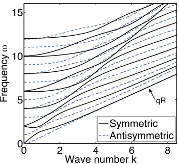
Fig. 2.2 Non-dimensionalized frequency spectrum, computed by Newton’s

Method, showing the first 10 symmetric (solid lines) and

an-tisymmetric (dashed lines) Lamb modes for a stress-free plate

with Poisson’s ratio of ν= .33 corresponding to aluminum. This

spectrum identifies the corresponding Lamb modes that could

be excited by the temporal frequency ω. qR identifies the region

of the spectrum corresponding to the quasi-Rayleigh waves that

are considered in the numerical applications of Section 4.2.3. . . 15

Fig. 3.1 Fourier continuation of the non-periodic function given byf(x) =

esin(5.4πx−2.7π)−cos(2πx)_. _{Red triangles/squares and blue circles} rep-resent d` = dr = 5 matching points and C = 25 continuation points, respectively. . . 22

Fig. 3.2 Numerical solution to the one-dimensional wave equation (3.23)

at times t = 0.5,0.6,0.7,0.8,0.9s based on use of Fourier

(11)

Fig. 3.3 Left: Maximum numerical errors over space and time for

solu-tions of the wave equation Dirichlet problem resulting from use

of FC and FD solvers over one full temporal cycle of a sinusoidal

solution with increasing number of wavelengths. Right:

Maxi-mum numerical errors resulting from use of the FC solver over

many temporal cycles for a five-wavelength traveling solution. . 31

Fig. 3.4 Same as Figure 3.3 but for the Neumann problem instead of the

Dirichlet problem. . . 32

Fig. 3.5 An example of a curvilinear mapping. . . 33

Fig. 3.6 Left: A portion of a physical domain covered by two patches

where the bold dots indicate the layers of interpolation points.

Right: One such curvilinear patch decomposed into four

sub-patches. . . 39

Fig. 3.7 One dimensional line segmentation analogous to the

multidimen-sional parallel decomposition of a patch. . . 41

Fig. 3.8 Left: A two-dimensional example of a square patch decomposed

into four disjoint sub-patches. Right: The four sub-patches

augmented by fringe regions and an example of the transmission

of data to corner patches. . . 42

Fig. 3.9 One dimensional line segmentation for periodic boundary

condi-tions. . . 43

Fig. 3.10 Depictions of the exponential filter with parameter values given by

(p, α) = (3N/5,16 log(10)) (left) and (p, α) = (4,−cL∆t/hminln(10−2)) (right). . . 47

Fig. 3.11 Numerical errors along thex-axis after 5000 time-steps for plane

waves in a thin plate of dimensions 70mm × 10mm ×25mm decomposed onto four sub-patches. Left: Errors for parameters

values (p, α) = (3N/5,16 ln(10)). Right: Errors for parameters

(12)

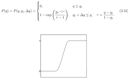
Fig. 3.12 An example of a stretching functionP(q). . . 52

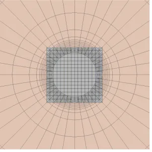
Fig. 3.13 An example of a square mesh overset by a radially absorbing

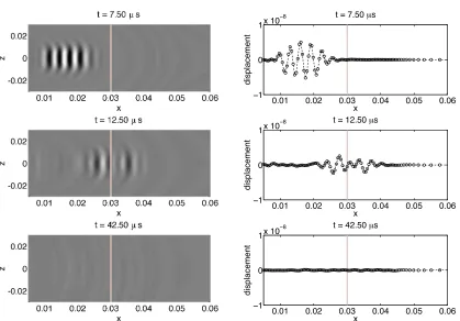
patch; γ0 = 0.10. . . 53 Fig. 3.14 A numerical simulation of the out-of-plane displacement resulting

from right-going waves traveling into an absorbing layer of

alu-minum (Nsponge = 100, γ0 = 0.075, β0 = 2) whose boundary is demarcated by the vertical line. The right-hand column of figures

represents the corresponding amplitude along the horizontal at

z = 0. . . 55

Fig. 3.15 Numerical values of the vertical displacement produced by the

right-hand-side source (3.57). The bold dots indicate the layers

of interpolation points used. . . 58

Fig. 3.16 From left to right: The numerical solution of equation (3.58)

at time t = 0.1s for configurations involving n = 3,12 and 48

wavelengths along a thin aluminum plate. . . 59

Fig. 3.17 Maximum numerical errors over all space and over one full

tem-poral cycle of a plane wave solution with increasing number of

wavelengths for Dirichlet (left) and traction (right) boundary

conditions. . . 60

Fig. 3.18 Numerical errors over many temporal cycles for a plate

ten-wavelengths in length demonstrating long-time stability for

Dirich-let and Traction boundary conditions (left and right images,

respectively). . . 61

Fig. 4.1 Left: Computational domain corresponding to a 180 meter hill

composed of two overset patches. Right: A two-dimensional

(13)

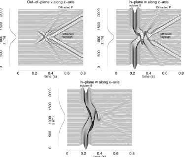
Fig. 4.2 Time responses of various displacement components on the

sur-face for receivers placed along the z-axis (the minor axis of the

mountain) and x-axis (the major axis). The incident S-wave is

polarized along the minor (z-) axis of the 180m mountain. . . 69

Fig. 4.3 Horizontal displacementw(x, y, z, t) at various snapshots in time,

where the z-coordinate direction contains the minor axis of the

hill. An intense field concentration at the summit is clearly visible,

as is the preferential propagation direction of the diffracted waves

(in the direction of the short axis of the mountain) it generates.

The time slider is given underneath each snapshot. . . 70

Fig. 4.4 Computational domain for a four steeply-sloped mountain system,

and corresponding overset patches. . . 71

Fig. 4.5 Time responses of various displacement components on the

sur-face for receivers placed along the z-axis andx-axis for a

topog-raphy consisting of a cluster of four sharp mountains. . . 73

Fig. 4.6 Horizontal displacementw(x, y, z, t) at various snapshots in time.

Much of the diffracted energy remains concentrated within the

cluster of hills long after impact. . . 74

Fig. 4.7 Model of an aluminum plate overset with a sponge layer. . . . 76

Fig. 4.8 An example of the windowing function S (black) given by (3.53)

and the resulting sinusoidal waveform (blue) for the incident

source. The center of the vertical axis represents zero amplitude. 77

Fig. 4.9 The amplitude of the numerical displacementv as a response to

a periodic source near the left edge of the displayed region. . . 79

Fig. 4.10 A snapshot of the P-wave-train displacement field arising from a

normally incident source at frequencies f = 1.8 MHz (left) and

(14)

Fig. 4.11 Experimental values for the modulus of the complex out-of-plane

displacement as depicted in [53] for the scattering of thin

waveg-uides in plates with through-hole defects. . . 80

Fig. 4.12 Experimental setup as depicted in [53] for generation and

record-ing of surface waves in a thin plate. . . 81

Fig. 4.13 Photographs of experimental samples including holes of circular

(left) and slot (right) shapes. . . 83

Fig. 4.14 Computational models corresponding to the experimental

geome-tries presented in Figure 4.13. The models are composed of six

overlapping patches (bottom row). . . 84

Fig. 4.15 Meshes for a rounded circular and rectangular scatterer that

are constructed by revolving two-dimensional grids produced by

means of the transfinite interpolation described in Appendix A. 85

Fig. 4.16 Experimental (left) and simulated (right) snapshots of the

inci-dent waves for the 12mm diameter circular hole. Top: real part of

the out-of-plane displacementv(x, y, z, t).Bottom: corresponding

complex amplitude. . . 86

Fig. 4.17 Experimental (left) and simulated (right) snapshots of the

scat-tered waves for the 12mm diameter circular hole. Top: The real

part of the out-of-plane displacement v(x, y, z, t). Bottom: The

corresponding complex amplitude. . . 87

Fig. 4.18 Horizontal and vertical cross-sections of the fields displayed in

Figure 4.16. . . 88

Fig. 4.19 Left: Peak modulus value of thevcomponent of the backscattered

field at point x using time as a parameter. Time advances right

to left. Right: Location of the peak modulus as a function of

time including the incident (Zone 1) and backscattered (Zone 3)

(15)

Fig. 4.20 Close-up of the 12mm diameter circular hole boundary for each

displacement componentu,vandw(from left to right, respectively)—

clearly visible are the waves flowing from the top surface to the

bottom along the hole thickness and the mode conversion between

the in-plane components u and w. . . 91

Fig. 4.21 Scattering results for the 4,6 and 8mm diameter circular hole

configurations (from top to bottom, resp.) for the displacement

components u,v and w. . . 92

Fig. 4.22 Snapshots of wave scattering by a 24mm long rectangular slot. 93

Fig. A.1 Left to right: examples of rounded edges constructed via

trans-finite interpolation between two lines, a quadratic B´ezier curve,

and a polar parameterization of the superellipse (A.1). . . 98

Fig. B.1 The 2D parametric slot geometry for use in the Helmholtz solver. 104

Fig. B.2 Results of the far field (right) as the slot height (left) is reduced

and the corners are successively sharpened. The last strip is that

of an open arc. . . 105

Fig. B.3 Time-harmonic scattering in 2D using the acoustic scalar equation

and Neumann boundary conditions. . . 106

Fig. D.1 Left: Two-dimensional example of an overlapping patch in thex-y

plane, where the red grid represents the interpolation stencil in an

annular patch and the green dot represents an interpolation point

in the rectangular patch. Right: The stencil and interpolation

point in the corresponding q-r plane of the annular donor patch

(16)

List of Tables

Table 3.1 Convergence results for the maximum error over all space and

time of the solution to the 1D wave equation (3.23). . . 30

Table 3.2 Maximum error in the elastic displacement over 5000 time-steps.

A fine temporal discretization is used so that the overall error is

dominated by errors arising from the spatial discretization. . . 58

Table 3.3 CPU-seconds per million unknowns and errors for a domain

consisting of a single curvilinear patch (no interpolation),

indi-cating excellent scalability up to at least 480 processors. Upper

table: weak convergence test, for which both the number of

dis-cretization points and the numbers of processors are increased

simultaneously. Lower table: strong convergence test, wherein for

a fixed number of grid points, the number of processors used is

in-creased. Clearly, essentially perfect parallel efficiency is obtained

(17)

Table 3.4 CPU-seconds per million unknowns and errors for a domain of

a plate with a circular-through hole consisting of six different

curvilinear meshes which interpolate from each other (see

Sec-tion 4.2.3). Upper table: weak convergence test, for which both

the number of discretization points and the numbers of processors

are increased simultaneously. Lower table: strong convergence

test, wherein for a fixed number of grid points, the number of

processors used is increased. Clearly, essentially perfect parallel

efficiency is obtained under weak and strong convergence tests. 64

Table 4.1 Reflection coefficients R for each hole diameter. . . 90

Table B.1 Surface density errors for the slot-through hole in 2D relative

to an“exact” solution usingN = 2048 discretization points. All

errors are absolute errors of the normalized solutions (maxv(r) = 1.)106

Table C.1 Domains for circular hole geometries. The boundary condition

for the incident field is applied to the left end of the interval for

x given in the third column. . . 108

(18)

Chapter 1 Introduction

I’m pickin’ up good vibrations... she’s giving me excitations...

- Brian Wilson and the Beach Boys

The energy introduced by a disturbance in a medium propagates, as traveling waves,

in a phenomenon that is familiar from everyday life, from seismic tremors in the earth

to ripples in a pond, and even the stylus that follows the spiral groove in a vinyl music

record—picking up these waves in the form of vibrations that travel along a metal

band at the end of the tone arm and that eventually convert to electrical signals that

are carried to an amplifier. The particular characteristics and information carried by

wave propagation—which may vary from medium to medium—can be quite complex,

having long been part of a great area of interest to theoreticians and experimentalists

alike, and having led to numerous mathematical models for propagation and scattering

of waves through gases, liquids, solids and free space [81, 26, 36, 39, 42, 61, 76].

Mechanical waves through a solid medium and, in particular, an elastic medium,

are the specific concern of this thesis and cover many interesting propagation

phe-nomena ranging in application from railroad rails to the seismic waves induced by

earthquakes which, for example, can travel thousands of miles all the while reflecting

and refracting through variations in the Earth’s surface and its underground

(19)

studies of elastic wave motion vary widely in applicability to many academic and

industrial problems, including the field of ultrasonics, which involves the introduction

of low energy, high-frequency wave packets into a material to determine fundamental

properties (such as elastic constants) or to detect particular defects (such as cracks or

holes)—all by measuring and analyzing the propagation, reflection and attenuation of

these pulses [53, 67, 11, 12, 70, 34]. (Further details will be provided in the context

of the specific material science problems considered in Chapter 4.) An excellent pair

of historical sketches and surveys of a great many other applications of elastic wave

propagation can be found in [3] and the classic text of [39].

1.1 Numerical PDE solvers for elastodynamics

The aforementioned elastic problems and associated wave motion, which are governed

by the equations reviewed in Chapter 2, present a host of challenges and difficulties

from a computational standpoint: the accurate, stable and dispersionless modeling and

computation of numerically stiff three-dimensional physical elastic systems—including

the treatment of curved stress-free surfaces, geometric singularities from corners and

edges, complex geometries and manifold other intricacies—is certainly considered

to be a highly challenging problem in computational science. These complexities

have motivated the development of a plethora of numerical models ranging widely in

accuracy and stability. Some well-established methods, such as discontinuous Galerkin

methods [46, 29, 47, 27] (developed for homogeneous materials where Lam´e material

parametersλ(x, y, z) =λ0 andµ(x, y, z) =µ0 are constant) and the (pseudo)spectral-element methods [32, 49], have been applied to the equations of elasticity with

arbitrary accuracy and with a sufficient treatment of complex geometries through

the use of unstructured grids. These methods, however, can have very restrictive

spectral radii—the timestep can scale quadratically or cubically with the spatial

mesh sizes. Additionally, to retain high-order approximations, the construction of

(20)

and un-automated manners. Alternative methods, such as extant finite difference

or finite element methods, both of which have been invoked to solve problems in

elasticity [7, 50, 72, 59] while still carrying CFL conditions that scale linearly, have

been well-known for a long time [60] to suffer from high numerical dispersion: errors

in the phase of a solution can accumulate over subsequent periods of the propagating

wave-train, demanding ever increasing numbers of points per wavelength to resolve,

within a given accuracy, increasingly larger problem sizes.

The Fourier-continuation based solvers considered in this work, which form the

foundation of the new numerical methodology we introduce in Chapter 3 for

elastody-namics problems, address all of these issues by extending Fourier series-based methods

to general, non-periodic domains—allowing for a less restrictive CFL condition as well

as a computation of derivatives in domain interiors that is spectrally accurate and

enables the method to be nearly dispersionless. As will also be demonstrated, this class

of solvers can be applied to arbitrary geometries and spatially varying (heterogeneous)

media while retaining high-order accuracy. Additionally, the advent and accessibility

of computing clusters makes possible a parallel implementation through use of Message

Passing Interfaces (MPI) by sharing the work and memory of solving problems in

large domains across many processors in a distributed computing environment—the

Fourier continuation framework herein lends itself naturally to implementation in such

computer hardware.

1.2 The elasticity solver developed in this thesis

This thesis represents a significant extension of the work by [4, 20, 54, 30, 21, 15, 17]

which, in the brief history of Fourier-continuation (FC) differentiation algorithms for

solution of Partial Differential Equations, introduces for the first time a full-fledged

three-dimensional solver that can be applied to arbitrary geometries for a complex

system of PDEs. In an effort to realize the potential of the Fourier continuation method

(21)

details our development and parallel computing implementation for a three-dimensional

model of a variable coefficient elastic wave equation including possibly heterogeneous

materials (that is, arbitrarily varying material parameters). The challenges of the

elastic Cauchy-Navier equation formulation we consider in this work—notably among

them the treatment of complex geometries including corners and edges, the enforcement

of physical surface boundary conditions by means of a modified FC operator introduced

in Section 3.1.2, and a number of stability concerns—are all addressed as part of this

work and are summarized within the general overview in what follows:

Chapter 2 reviews the physics and governing mathematics of elasticity theory, the displacement formulation of the elastic wave equation, and relevant physical

boundary conditions. Guided wave theory, where wave motion is directed by

what is known as a traction-free boundary condition, will also be discussed briefly

to provide some context for the material science and seismology applications

considered in Chapter 4. A scalar model for the out-of-plane displacement in

some of the non-destructive evaluation problems considered is also presented.

This work, which is based on use of the high-order integral equation solver

described in Appendix B, was published in [53] and is summarized briefly in

Section 4.2.

Chapter 3 extends the Fourier continuation methodology to general, arbitrary over-lapping curvilinear geometries in order to accommodate the geometric

com-plexities that include engineering detail (e.g. the real experimental setups

of defects in 3D plates modeled in Section 4.2.3) while retaining the spatial

high-order accuracy and stability of FC, and to enable implementation in a

fully parallel computational infrastructure. A description of the accelerated,

FC(Gram) method is presented in full detail, and it is extended to introduce, in

Section 3.1.2, a modified FC(Gram) operator suitable for Neumann and traction

boundary conditions as part of the general treatment prescribed in Section 3.3.3

(22)

coordinate version of the elasticity equations and traction boundary conditions,

which contain 189 and 21 spatial derivative terms, respectively, is formulated

in such a way as to enable treatment of general geometries by means of overset

patches—allowing for explicit interpolation of high-order of accuracy among

possibly hundreds of curvilinear sub-patches. These sub-patches are subsequently

assigned to computing processors by a simple load balancing algorithm, presented

in Section 3.2.3.3, for efficient implementation in distributed-memory parallel

environments. Stability issues and treatments of absorbing boundary conditions

(to enable approximation of unbounded domains) are additionally addressed in

this chapter.

Chapter 4 demonstrates the new solver in a variety of scientific and engineering contexts relevant to problems in materials science and seismology. In Section 4.2,

we will present, for the first time, a thorough comparison between experimental

scattering patterns of guided ultrasonic quasi-Rayleigh waves in plates with

through-thickness defects and fully three-dimensional elastodynamics numerical

simulations. Special consideration will be given to the geometry construction of

the respective experimental setups and, in particular, corners and edges will be

treated by means of a transfinite interpolation (Appendix A) and the overset

(23)

Chapter 2 The mathematical and physical

framework

The mathematics of continuum mechanics concerns the description of the mechanical

behavior of materials (e.g. solids, fluids, gases) under the action of forces and a

fundamental assumption that the respective material is modeled as a continuum. For

a solid material, external forces result in an internal restoring force (stress) given by

the (symmetric) stress tensor

σ =      

σ11 σ12 σ13

σ12 σ22 σ23

σ13 σ23 σ33       . (2.1)

The motion of a point in a material sitting at (x, y, z)T _{for a certain initial time} _t ₌_t 0 can be described by its displacement to a new position (˜x(x, y, z, t0+ ∆t),y˜(x, y, z, t0+ ∆t,z˜(x, y, z, t0+ ∆t))T by means of the displacement vector (u, v, w)T:

      ˜ x ˜ y ˜ z       =       x y z       +      

u(x, y, z, t)

v(x, y, z, t)

(24)

Using the notation fx = ∂f /∂x, fxx = ∂2f /∂x2 for derivatives, the gradient tensor

∇u of the displacement vector u= (u, v, w)T _{is given by}

∇u=      

ux uy uz

vx vy vz

wx wy wx

     

. (2.3)

The relative deformation induced by stresses given by the tensor (2.1) can be described

using the Green-Lagrange strain tensor E, which is related to the displacement gradient (2.3) by the expression

E= 1

2[∇u+ (∇u) T

+∇u·(∇u)T]. (2.4)

Materials elastic in nature, that is, that return to their original shape after deformation,

are generally governed by a non-linear constitutive law describing the relationship

between the stress σ given in (2.1) and the strain tensor E given in (2.4). (Other formulations, such as for hyperelastic materials, derive the stress-strain relationship

from an energy density function.)

2.1 Linear elasticity

This thesis is concerned with linear elasticity: small elastic deformations that can be

accurately described under linearization of the general non-linear laws that govern

elastic bodies. Under such assumptions the third term in the strain tensor (2.4) can be

neglected and an approximate deformation can be defined by the infinitesimal strain

(25)

ε =      

ε11 ε12 ε13

ε21 ε22 ε23

ε31 ε32 ε33       =        ux 1

2 uy+vx 1

2(uz+wx) 1

2 vx+uy

vy

1

2 vz+wy 1

2(wx+uz) 1

2 wy +vz wz        . (2.5)

Linear elasticity further provides a linear relationship, known as Hooke’s law,

between the stress σ and the infinitesimal strain tensor ε. For a linear isotropic material in the framework of this theory, there is no preferred direction in Hooke’s

law and the components ofσ are linearly related to components of ε through certain material constants λ and µ(known as Lam´e parameters); in such cases Hooke’s law

takes the form

σij =λδijεkk+ 2µεij, (2.6)

where δij is the Kronecker delta given by a value of δij = 1 when i=j and δij = 0 when i6=j.

2.1.1 The Cauchy-Navier equations for displacement

For an isotropic linear elastic solid contained in a domain Ω, the momentum-balance

equation in Cartesian coordinates, together with (2.6), becomes the system of Partial

Differential Equations given by [79]

ρutt =

h

(λ+ 2µ)ux+λ(vy+wz)

i

x+

h

µ(vx+uy)

i

y+

h

µ(wx+uy)

i

z+f1,

ρvtt =

h

(λ+ 2µ)vy +λ(ux+wz)

i

y+

h

µ(vx+uy)

i

x+

h

µ(vz +wy)

i

z+f2,

ρwtt =

h

(λ+ 2µ)wz+λ(ux+vy)

i

z+

h

µ(wx+uz)

i

x+

h

µ(wy+vz)

i

y+f3,

(2.7)

where f = f(x, y, z, t) is a vector of body forces. The material properties are given by the Lam´e parameters µ= µ(x, y, z), λ= λ(x, y, z) and the densityρ= ρ(x, y, z),

(26)

λ(x, y, z) =λ and µ(x, y, z) =µ are constant, Equation (2.7) can be written as

ρu¨=µ∇2u+ (λ+µ)∇∇ ·u+f, (x, y, z)∈Ω, (2.8)

where u= (u, v, w)T_.

The initial displacement and velocities at an initial time t =t0 must be prescribed:

u(x, y, z, t0) =a1(x, y, z), ut(x, y, z, t0) = b1(x, y, z),

v(x, y, z, t0) =a2(x, y, z), vt(x, y, z, t0) =b2(x, y, z),

w(x, y, z, t0) =a3(x, y, z), wt(x, y, z, t0) =b3(x, y, z).

(2.9)

Boundary conditions must also be given, as discussed in the following section.

2.1.2 Boundary conditions

On the boundary ∂Ω of a solid geometry, different forms of data can be imposed for

the elastic wave equation to model physical configurations. The traction boundary

condition, which prescribes the normal stresses on the solid boundary, is given by

     

σ11 σ21 σ31

σ12 σ22 σ32

σ13 σ23 σ33             n1 n2 n3       =      

d1(x, y, z, t)

d2(x, y, z, t)

d3(x, y, z, t)      

on ∂Ω, (2.10)

where [n1, n2, n3]T is the inward unit normal on the surface andd1, d2, d3 are functions of the spatial coordinates and time. In terms of displacements, the traction boundary

conditions can be made to read

(2µ+λ)ux+λ(vy+wz)

n1+µ

vx+uy

n2 +µ

wx+uz

n3 =d1(x, y, z, t),

µvx+uy

n1+

(2µ+λ)vy+λ(ux+wz)

n2 +µ

wy+vz

n3 =d2(x, y, z, t),

µwx+uz

n1+µ

wy+vz

n2+

(2µ+λ)wz+λ(ux+vy)

(27)

Many applications—and in particular, those in this work—involve traction-free (or

free-surface) boundary conditions. These are characterized by vanishing normal stresses

on the surface of the domain, i.e. d1(x, y, z, t), d2(x, y, z, t), d3(x, y, z, t)≡0.

A Dirichlet boundary condition can also be imposed as data on the displacements

u, v, w at a boundary as

u=c1(x, y, z, t), v =c2(x, y, z, t), w=c3(x, y, z, t) on ∂Ω. (2.12)

It is often necessary to additionally utilize techniques that enable simulation of an

actually infinite medium by means of a bounded computational domain. In this thesis

this is accomplished by resorting to use of certain sponge regions (absorbing layers)

surrounding the actual physical domain. In the sponge layers we employ, both the

computational domain is stretched outside the region of interest and a corresponding

numerical dissipation term is added to the system of PDEs to dampen the amplitude

of the displacements. Details regarding these are provided in Section 3.3.4.

2.2 Longitudinal and transverse waves

A Helmholtz decomposition of the displacement vector (u, v, w)T _{into a scalar potential}

φ(x, y, z, t) and a vector potential ψ(x, y, z, t) in the form

(u, v, w)T ₌_∇_φ₊_{∇ ×}_ψ _(2.13)

yields from Equation (2.8), for constant material parameters λ(x, y, z) = λ0 and

µ(x, y, z) = µ0, the expression given by

ρ∂

2

∂t2[∇φ+∇ ×ψ] = [µ∇

(28)

Noting the fact that ∇ · ∇φ =∇2_φ _and_{∇ · ∇ ×}_ψ _{= 0 and in absence of the body} forces, a rearrangement of this equation yields

∇[(λ+ 2µ)∇2φ−ρφtt] +∇ ×[µ∇2ψ−ρψtt] = 0. (2.15)

Clearly, this equation is satisfied provided a corresponding pair of wave equations,

namely, the scalar wave equation

φtt =c2L∇2φ, (2.16)

with the longitudinal wave speed

cL =

s

λ+ 2µ

ρ , (2.17)

and the vector wave equation

ψ_tt =c2T∇2ψ, (2.18)

with the transverse (shear) wave speed

cT =

r_µ

ρ (2.19)

are satisfied. The wave speeds (2.17) and (2.19) (which only depend on the material

parameters ρ, λ and µ) satisfy the relation

cL

cT =

r

2(1−ν)

1−2ν , (2.20)

where ν = λ

2(λ+µ) denotes the material’s Poisson’s ratio.

The solutions φ to the scalar wave equation (2.16) are known as P-waves (or

pressure waves, or longitudinal waves): they involve wave motion of particles in the

(29)

vector wave equation (2.18) are commonly known as S-waves (or shear waves, or

transverse waves) whose motion is contained in any direction of a plane normal to

the direction of propagation. Motion of S-waves can be horizontally (SH-waves) or

vertically (SV-waves) polarized; for example, in the aluminum plates considered in

this thesis, an SH-wave travels within the plane of the plate and an SV-wave travels

through its thickness. For a more extensive review of the many sorts of waves, we

refer to the textbooks [3, 42, 39, 36, 76].

2.3 Guided-wave theory

The bulk waves that travel through the interior of a solid are characteristically

non-dispersive, that is, cL andcT are functions ofρ, λ andµ, only: they do not depend on frequency. However, mechanical waves can also propagate along an interface between

media of different acoustic impedances: these are known as surface waves. When one

of the two media is a vacuum, surface waves are simply guided by vanishing stress

(traction-free) boundary conditions. Unlike bulk waves, these waves are dispersive in

nature (wave speed is a function of frequency) and exhibit an infinite number of wave

modes.

In seismology, surface waves are commonly categorized as either Love waves or

Rayleigh waves. Love waves, which were predicted mathematically by A. E. H. Love,

are SH-waves guided by an elastic layer (an elastic half space bordered by a vacuum)

and decay within the depth of the layer. These waves cause the horizontal shifting

observed during an earthquake and travel, for typical homogeneous elastic media, at a

speed that is around 90% of the transverse wave speed cT.

Rayleigh waves, which were predicted by Lord Rayleigh in 1885, carry both a

longitudinal and transverse motion along the surface of a semi-infinite elastic solid

and are slightly slower than Love waves. Ever-present in earthquakes, these waves

can also be produced by piezo-electric transduction or by a localized impact, and

(30)

Figure 2.1: A thin plate.

neither material on each side of an interface is a vacuum, Rayleigh waves are also

called Stoneley waves (if the two materials are solids) or Scholte waves (if one is

a liquid and the other a solid). When guided in layers, Rayleigh waves are called

generalized Rayleigh waves orLamb waves—they travel through the body and along

both traction-free surfaces of a thin plate or shell.

Lamb wave theory [42, 52, 64, 55, 56, 57]—also known as “plate theory”—was

pioneered by its namesake Sir Horace Lamb at the turn of the 20th century [52] and

is of great practical interest to the non-destructive techniques introduced in the next

section and modeled in Chapter 4. It considers a plate, illustrated in Figure 2.1, of

infinite extent in thex andz coordinate directions. The plate has a finite thickness of

2h in the y coordinate direction and is under conditions of plain-strain: traction-free

surfaces at y= ±h. In light of the rectangular geometry, the corresponding boundary condition (2.11) reduces to the system given by

σ21= 0 =µ(vx+uy),

σ22= 0 = (2µ+λ)vy +λ(ux+wz),

σ23= 0 =µ(wy+vz).

(2.21)

Solutions to this problem can be expressed in terms of two sets of modes: 1) symmetric

modes, where displacement in thex-direction is symmetric to the midplane of the plate;

and, 2) antisymmetric modes, where displacement in the x-direction is anti-symmetric

(31)

general solutions

φ = Φ(y) exp(ikx−ωt),

ψ =Ψ(y) exp(ikx−ωt),

(2.22)

of the uncoupled wave equations (2.16) and (2.18), whereωis the angular frequency and

k its corresponding wave number, the displacement solutions for both the symmetric

and anti-symmetric cases are of the form [2, 39]

u=i(Bξcos(αy) +Cβcos(βy))ei(x−ωt)_,

v = (−Bαsin(αy) +Cξsin(βy))ei(x−ωt)_, (2.23)

and, respectively,

u=i(ξAsin(αy)−Dβsin(βy))ei(x−ωt)_,

v = (Aαcos(αy) +Dξcos(βy))ei(x−ωt)_, (2.24) whereα2 = ω2/c2_L−k2 andβ2 = ω2/c2_T−k2.An application of the boundary conditions given by (2.21) yields the well-known dispersion relation between the angular frequency

ω and the corresponding wavenumber k given by

tan(βh) tan(αh) =−

4αβk2 (k2₋_β2₎2

!±1

,

      

+1 symmetric

−1 antisymmetric

, (2.25)

and known as the Rayleigh-Lamb frequency equations for a thin plate. Solutions

to the highly non-linear equations of (2.25) were once considered intractable, but

computers have enabled calculations of the full frequency spectrum in a reasonable

amount of computational time, as we have done in Figure (2.2) via a simple application

of Newton’s Method [62]. For the non-destructive applications considered in later

chapters, the region of excitation for the incident fields induced in the experimental

samples of sufficiently thick plates is located at the upper end of the zeroth symmetric

and anti-symmetric modes of the spectrum displayed in Figure 2.2; in this region—

(32)

can also be described asquasi-Rayleigh waves [67, 78]: the phase and group velocities

are close to the phase velocity of the Rayleigh wave and the distribution through the

upper and lower halves of the plate mimic that of a Rayleigh wave as well.

0 2 4 6 8

0 5 10 15

Wave number k

Frequency

t

Symmetric Antisymmetric

[image:32.612.230.405.189.350.2]

qR

Figure 2.2: Non-dimensionalized frequency spectrum, computed by Newton’s Method, showing the first 10 symmetric (solid lines) and antisymmetric (dashed lines) Lamb modes for a stress-free plate with Poisson’s ratio of ν =.33 corresponding to aluminum. This spectrum identifies the corresponding Lamb modes that could be excited by the temporal frequency ω. qR identifies the region of the spectrum corresponding to the quasi-Rayleigh waves that are considered in the numerical applications of Section 4.2.3.

2.3.1 Scalar model

As discussed above, Lamb modes are described using scalar and vector potentials in

(2.22), but an alternative decomposition introduced by [2, 3] can be used to describe

the modes with one scalar potential φ superposed with carrier waves (one-dimensional

functions V(y) and W(y) in the thickness of the plate) that act as “membrane-like

(33)

to (2.8) for each mode of the form

u(x, y, z, t) = 1

kV(y)e

iωt ∂

∂xφ(x, z), v(x, y, z, t) =W(y)eiωt_φ₍_{x, z}₎_,

w(x, y, z, t) = 1

kV(y)e

iωt ∂

∂zφ(x, z),

(2.26)

where V(y) and W(y) are smooth functions in the thickness dimension of the plate

that characterize transversal shapes for a given mode. The function φ(x, z) satisfies

the two-dimensional Helmholtz equation

∇2φ+k2φ= 0 (2.27)

in the plane given byxandz. For a given moden, then, it follows that aty= constant,

the out-of-plane displacement v(x, y, z, t) satisfies the equation

∇2v +k2v = 0 (2.28)

for the wave number k which, for plates, is given by the Rayleigh-Lamb frequency

equation (2.25). The decomposition given by (2.26) prompted the work [53], in which

a two-dimensional scalar potential was used to approximately model through-thickness

defects using the time-harmonic acoustic equation—the geometry depends only on the

(x, z) coordinates and in a sense is two-dimensional. Scattering that was produced

under conditions where only one propagating mode contributed to v enabled the use

of (2.28), supplemented by a Neumann boundary condition, as a first approximation

(see Appendix B). The validity of this model was justified in [53] “a posteriori on the

basis of comparison of model results with experimental data,” but, as demonstrated in

Chapter 4, this approximation, while in fairly good agreement, does not fully capture

(34)

Chapter 3 A new methodology for solving the

elastic wave equation

This chapter presents a high-performance numerical methodology for the solution of

elastodynamics problems. Based on a certain “Fourier continuation” (FC) approach

for accurate Fourier expansion of possibly non-periodic functions [20], the proposed

methodology possesses a number of appealing properties: it yields essentially

disper-sionless results, it gives rise to CFL constraints that scale only linearly with the spatial

mesh sizeh, it runs at a cost that scales linearly with the discretization sizes, and it

lends itself easily to parallelization in distributed-memory computing clusters. The new

FC algorithm, which applies to a great many problems in elastodynamics, including

general geometries and possibly heterogeneous and spatially varying elastic constants,

is demonstrated in this thesis via a number of applications to problems concerning

ma-terials science and, more specifically, non-destructive evaluation. Our FC treatment of

the elastic (Cauchy-Navier) equations is based on the high-order-accurate FC method;

other extant FC-based PDE solvers include solvers for the classical wave and diffusion

equations [20, 54, 21, 30] as well as the compressible Navier-Stokes equations [4].

The development described in this thesis of FC solvers for elastic wave-propagation

problems represents an important extension of the FC methodology: the equations

pose a number of significant challenges concerning stability, enforcement of boundary

(35)

3.1 The treatment of spatial derivatives

In view of their simplicity, classical differentiation methods such as those based on use of

finite differences or finite elements are often used as part of PDE discretization schemes.

As is well known, however, Finite Difference (FD) and Finite Element Methods (FEM)

for PDEs governing wave-like phenomena do give rise to high numerical dispersion:

phase errors accumulate over subsequent periods of a wave field, and thus FD and FEM

solvers require increasing numbers of discretization points per wavelength to resolve

the solution within a given accuracy tolerance as the size of the problem grows. As is

well known, methods based on use of Fourier series do not suffer from this problem:

a fixed number of discretization points per wavelength suffices to produce wave-like

solutions with a fixed accuracy in domains containing arbitrarily large numbers of

waves (up to the wavenumber associated with the finest resolution).

Unfortunately, however, classical Fourier methods are only applicable to periodic

functions—since Fourier expansion of a non-periodic functions gives rise to the

well-known “ringing effect” (the Gibb’s phenomenon [38]): the jump that results in the

periodic extension of an inherently non-periodic function leads to an “overshoot” in

the Fourier representation at points of discontinuity of the periodic continuation of

the given function. This inaccuracy does not subside as more terms are added and, in

fact, it results in extremely slow pointwise convergence throughout the interior of the

computational domain—in addition to the unmitigated error at domain boundaries.

A goal to extend the applicability of Fourier methods (together with its inherent

excellent qualities, most notably dispersionless-ness and high-order accuracy) to general

non-periodic configurations has lead to the development of the FC methods that play

a central role in this thesis. The Fourier continuation (FC) method produces a

rapidly-convergent interpolating Fourier series representation of a given function on a region

larger than the given physical domain. This is accomplished by relying on a “periodic

extension” of the given function, that closely approximates the given function values

(36)

and thus suitable for Fourier approximation. In detail, given a function f which is

defined, without loss of generality, on the unit interval as

f(x) : [0,1]⊂_R→_R,

the FC method produces a periodic function fc _{defined on an extended interval,}

fc₍_x_{) : [0}_{, b}_]_⊂

R→R, b >1

which closely approximates f(x) on the original interval [0,1].

Fully discrete Fourier continuation algorithms generally proceed as follows: letting

N be the number of discretization points over the unit interval (yielding a uniform

grid xi = ih, i = 0, . . . , N −1, h = 1/(N −1)) together with point values f(xi) of the function of interest, the Fourier continuation method produces a b-periodic

trigonometric polynomial fc _{of the form}

fc₍_x_{) =} M

X

k=−M

ake

2πikx

b , (3.1)

that matches the given discrete values off: fc₍_x

i) =f(xi), i= 0, ..., N−1.Derivatives of the function can then be easily computed through term-by-term differentiation, e.g.

fx(x) = fxc(x) =

M

X

k=−M

2πik b

ake

2πikx b ,

fxx(x) = fxxc (x) = − M

X

k=−M

2πk2 b2

!

ake

2πikx b ,

.. .

(3.2)

In the simplest treatment [18, 15, 17], the coefficients ak of (3.1) are found by invoking the Singular Value Decomposition to solve the least squares system

min ak N−1 X i=0

fc(xi)−f(xi)

(37)

Although straightforward, repeated applications of the SVD for time-dependent

func-tion values on each line of a three-dimensional mesh in a PDE is, in general,

unac-ceptably costly. To circumvent this difficulty, an accelerated method was proposed in

[20, 54] which allows for Fourier continuation of functions on the basis of a number of

d=d`, dr end function values at the left and right intervals and a projection onto a Gram polynomial basis whose FC extensions are precomputed via a high-precision

SVD. In effect, this procedure produces a “basis” of continuation functions that can

be utilized by a PDE solver. The technique was modified in [4] into a “biased-order”

algorithm appropriate for high-performance computing including domain

decomposi-tion. The latter “FC(Gram)” method is described in Section 3.1.1 and extended in

Section 3.1.2 to a form suitable for our elasticity solver.

3.1.1 Accelerated Fourier continuation: FC(Gram)

Given a column vector f = (f0, . . . , fN−1)T containing N values of a given function

f in its domain [0,1], fi = f(xi) (0 =x0 < x1 < · · · < xN−1 = 1), the accelerated FC(Gram) method [20, 54, 4] uses a subset of the given function values on small

numbers d` and dr of matching points {x0, .., xd`−1} and {xN−d, ..., xN−1} contained in small subintervals on the left and right ends of the interval [0,1] (of lengths

δ` = (d`−1)h andδr = (dr−1)h) to produce, at first, a discrete periodic extension. Using such data, the FC(Gram) algorithm thus appends a number C of continuation

function values for the periodic extension in [1, b] to transition smoothly fromfN−1 back to f0; see Figure 3.1. The resulting vector fc can be viewed as a discrete set of values of a smooth and periodic function which is suitable for high-order approximation

by means of the FFT algorithm in an interval of length (N+C)∆x.

In order to evaluate the C necessary extension values mentioned above, the

accelerated FC(Gram) method uses the given functionf defined in the interval [0,1]

together with a translation of it by a distance b. Defining the sets D` ={b+x0, b+

(38)

the interval [1, b] are obtained as point values of an auxiliary trigonometric polynomial

of periodicity interval [1−δr,2b−(1−δr)] (with appropriately selected bandwidth) which closely approximate the function values on Dr ∪ D`. This approximating trigonometric polynomial is obtained as the result of a two-step process, namely 1)

projection onto bases of orthogonal polynomials, and 2) continuation through use of a

precomputed set of continuations-to-zero of each Gram polynomial, as explained in

what follows.

The polynomial projection mentioned in step 1) above for the function values on

Dr∪D` relies on use of two Gram (orthonormal) bases, Br and B`, of the respective spaces of polynomials of degree < d`, dr on the intervals [1−δr,1] and [b, b+δ`] with respect to the natural discrete scalar product defined by the discretization points Dr and D` [20, 54] (see Equation (3.9) below). The algorithm also utilizes precomputed extensions, one for each polynomial pr ∈ Br, into a smooth function defined for

x ≥ 1−δr, which approximates pr closely in the matching interval [1−δr,1], and which blends smoothly to zero for x ≥ b. Such rightward extension is obtained by means of appropriately oversampled least squares approximations by Fourier series of

periodicity interval [1−δr, b−(1−δr)], as described in [20, 54]. Similarly, the scheme obtains, for each polynomial p` ∈B`, a smooth blending function that agrees with p` in the matching interval [b, b+δ`] and which vanishes for x≤1.

In presence of such smooth blending, step 2) proceeds: an FC extension is

pro-duced, for the given function, from its values at the set of points Dr∪D`—since the interpolating polynomials of degree dr−1 on Dr andd`−1 onD` can be expressed as linear combinations of the polynomials in the bases B` and Br, with coefficients that can be obtained rapidly by means of scalar products. With the extension in hand,

an application of the discrete Fourier transform on the interval [0, b] to the vector

of function values f augmented by the C “continuation” values yields the desired trigonometric polynomial (3.1). An example of the blending procedure is depicted in

(39)

0 .5 1 b 1.5 2 0 2 4 6 f Af f! fr

dr = 5

d!= 5

C = 25

Figure 3.1: Fourier continuation of the non-periodic function given by f(x) = esin(5.4πx−2.7π)−cos(2πx). Red triangles/squares and blue circles representd`=dr= 5matching points andC= 25continuation

points, respectively.

The resulting continuation operation can be expressed in a block matrix form as

fc₌

   I A   f =

   f Af  

, (3.4)

where fc _{is a vector of the} _N ₊_C _{continued function values,} _I _{is the} _N _×_N _identity matrix and A is the matrix containing the blend-to-zero continuation information.

Defining the vector of matching points for the left and right as

f` =

         f0 f1 ...

fd`−1         

, fr =

        

fN−dr

fN−dr+1 ...

fN−1          , (3.5)

gives anAf of the form

Af =A`QT`f`+ArQTrfr, (3.6)

(40)

corresponding Gram polynomial basis, and where the columns of A` and Ar contain the correspondingC values that blend the left and the right bases to zero. For d` =dr the matrices A` and Ar (resp. Q` and Qr) differ only by row-ordering (resp. only by column ordering). The matrices Q=Q` and Q=Qr for given numbers d=d` and

d=dr of matching points may be obtained by orthogonalizing thed×d Vandermonde matrix

P =

        

1 x0 (x0)2 ... (x0)d−1 1 x1 (x1)2 ... (x1)d−1

... ... ... ... ... 1 xd−1 (xd−1)2 ... (xd−1)d−1

        

, (3.7)

of point values of the monomialsxj (j = 1, . . . , d−1) at the discrete pointsx0, x1, ..., xd−1. (A substitution of x by (x−1) must be used for the right matching problem.) This is

performed by applying a Gram-Schmidt orthogonalization process

P =QR (3.8)

with respect to the inner product

(g, h)r=

X

xi∈Dr

g(xi)h(xi), (3.9)

and a similar inner product for (g, h)`,where thejth column ofQin (3.8) contains the

d point values of the jth Gram basis polynomial. To ensure a good agreement with

the constraints described by the least squares problem introduced in what follows, we

additionally oversample the monomial basis by a factor ofnover = 20, which leads to a Vandermonde matrix Pover _{similar to (3.7) but of size (}_n

over(d−1) + 1)×d. The corresponding matrix whose columns are the Gram basis polynomials evaluated on a

grid nover times finer can be reconstructed by

(41)

where R is the upper triangular matrix in the orthogonalization of the coarse P

in (3.8).

Remark 1. The ill-conditioning of the full continuation problem is concentrated here

at the orthogonalization of the poorly conditioned Vandermonde matrix (3.7); such a

decomposition is well known to possibly suffer from a numerical loss of orthogonality.

This difficulty is addressed by relying on high-precision (using 256 digits) and symbolic

arithmetic throughout the process of evaluation of precomputed continuations for the

polynomial basis elements. This is an operation that needs to be performed only once

and stored in file for use each time the Fourier continuation is invoked. Technical

details concerning the implementation of this high-precision precomputation procedure

can be found in Appendix D.

Letting Z be the number of zero points used for the blending and letting E be a

certain number of additional points that are used to allow for continuation regions of

user-prescribed lengths, we define the intervals

Imatch = [0,(d−1)∆x],

Iblend= [(d−1)∆x,(d+C−1)∆x],

Izero= [(d+C−1)∆x,(d+C+Z −1)∆x],

Iextra = [(d+C+Z−1)∆x,(d+C+Z +E−1)∆x]

(3.11)

which contain d, C, Z and E discretization points, respectively. The function that

blends the discrete values of a given Gram polynomial on Imatch to the zero function values inIzero is obtained as a band-limited trigonometric polynomial

f(x) = M

X

k=−M

ake

2πikx

(d+C+Z+E−1)∆x (3.12)

that matches closely (in a least-squares sense) the Gram polynomials and an interval

(42)

a = (a−M, ..., aM)T are found by solving the minimization problem (posed on the oversampled Gram basis Qover _{with columns} _qover

k in (3.10)) given by

min

a=(a−M,...,aM)T

Bover_a₋

   qover j 0    2 , (3.13)

where Bover is a matrix formed from values of the function (3.12) at the ∆x/nover discretizations of Imatch and Izero, and where 0 is the zero vector of length (Z − 1)nover+ 1. The minimizing Fourier coefficients a= (a−M, ..., aM)T in (3.13) are then found by a Singular Value Decomposition and, once determined, the corresponding

columns of A`, Ar are constructed by evaluating (3.12) on the coarse discretization ∆x of the full continuation interval [0,(d+C+Z +E−1)∆x].

Remark 2. For all computations in this thesis, the parametersC = 25, Z = 12, E = 25

and nover = 20 were used to construct continuations for various integer values of d=

d`, dr. These choices were made in accordance with previous FC-based algorithms [4,

30], and were determined empirically to provide an appropriate trade-off between

computational cost in a PDE solver and stability of the operator constructed by the

above procedure.

3.1.2 A modified accelerated FC operator for Neumann

bound-ary conditions

In order to treat Neumann boundary conditions (and, ultimately, traction boundary

conditions), a modified version of the accelerated (biased-order) algorithm described in

Section 3.1.1 is needed to construct an operator appropriate to match the values of the

derivative of a functionf at the end pointxd−1 in addition to values off atx0, ..., xd−2. A simple extension of the algorithm presented above can be made to achieve this goal.

Indeed it suffices to use a polynomial interpolant that, in particular, matches the

(43)

the modified Vandermonde matrix

Pder =

        

1 x0 (x0)2 ... (x0)d−1

... ... ... ... ...

1 xd−2 (xd−1)2 ... (xd−2)d−1 0 1 2xd−1 ... (d−1)(xd−1)d−2

        

(3.14)

instead of (3.7) by means of the (high-precision) QR-decomposition

Pder =QderRder. (3.15)

The modified Fourier continuation blend-to-zero information can be obtained in

two ways, both of which in practice have been found to give the same results: 1) by

proceeding to form a new continuation basis in a manner analogous to Section 3.1.1,

replacing Q with Qder and the appropriate Bover with a corresponding Bderover in the least squares formulation; or, 2) by reconstructing the coefficients in the original

Gram polynomial basis and simply replacing the operator Q (= Q`, Qr) in (3.6) with a new operator ˜Q (= ˜Q`,Q˜r) for which the same pre-constructed blend-to-zero Dirichlet operators A`, Ar obtained in the previous section can be employed. The latter method—which is used in this work and introduced in what follows—carries the

advantage that the Gram polynomials blending-to-zero data computed in the previous

section, which was produced in the context of Dirichlet boundary conditions, may be

(44)

The construction of ˜Q is obtained by solving the system Pder             c0 c1 ...

cd−1

cd−1             =             f0 f1 ...

fd−2

f0(xd−1)

            . (3.16)

for the coefficients in (3.16) via the decomposition (3.15) as

            c0 c2 ...

cd−2

cd−1            

=R_der−1QT der             f0 f1 ...

fd−2

f0(xd−1)

            . (3.17)

Recalling the Vandermonde matrixP and its QR-decomposition in (3.8), substitution

of these coefficients into

P             c0 c2 ...

cd−2

cd−1             =QR             c0 c2 ...

cd−2

cd−1             =             f0 f1 ...

fd−2

fd−1             (3.18)

(45)

QRR−_der1QT der             f0 f1 ...

fd−2

f0₍_x d−1)

            =             f0 f1 ...

fd−2

fd−1            

⇐⇒ Q˜T

            f0 f1 ...

fd−2

f0₍_x d−1)

           

=QT

            f0 f1 ...

fd−2

fd−1             (3.19)

for ˜Q= (RR−_der1QT

der)T. Hence the continuation procedure constructed in the previous section and embodied in the formula

Af =A`QT`f`+ArQTrfr (3.20)

is modified by substitution of (3.19) into (3.20) to yield

Af =A`Q˜T`˜f`+ArQ˜Tr˜fr, (3.21)

where ˜f`= (f0, ..., fd`−2, f 0

(xd`−1)) T_,˜_f

r = (fN−dr, ..., fN−2, f 0

(xN−1))T and whereA`, Ar are the same blend-to-zero operators. Note that if, for example, one requires the

continuation to approximate the valuef(x0) and the derivative f0(xN−1) (as is often necessary as a result of the domain decomposition strategy that we introduce later in

this thesis), one needs only to form the corresponding biased continuation using the

appropriate projections on the left and the right as

Af =A`QT`f`+ArQ˜Tr˜fr, (3.22)

(46)

3.1.3 A simple preliminary 1D example with Dirichlet and

Neumann boundaries

As a simple example to verify the character of the FC methodology for both Dirichlet

and Neumann problems, consider a 1D wave propagation problem with initial values

given by a Gaussian profile:

      

utt(x, t) = uxx(x, t),

u(x,0) =e−300(x+.5)2 .

(3.23)

In order to facilitate evaluation of errors in our Dirichlet and Neumann test cases, we

set up Dirichlet and Neumann boundary conditions at x= 0 and x= 1 in such a way

that the exact solution is given by the traveling wave function

u(x) =e−300(x−ct+.5)2

, 0≤x≤1, (3.24)

which is depicted in Figure 3.2.

0 0.2 0.4 0.6 0.8 1

0 0.5 1

x

u

Figure 3.2: Numerical solution to the one-dimensional wave equa-tion (3.23) at times t= 0.5,0.6,0.7,0.8,0.9s based on use of Fourier continuation (d` = dr = 5, C = 25,∆x = 1/100) and explicit time

marching (∆t= ∆x/32).

Using the FC method for evaluation of spatial derivatives, and utilizing the explicit

fourth-order Adams-Bashforth method to evolve the resulting set of ODEs, we obtain

a PDE solver for the wave equation (3.23). Using a small time-step enables us to

(47)

mesh sizes. Table 3.1 displays, for both the Dirichlet and Neumann problems, the

maximum error over all spatial points x ∈[0,1] and for all times between 0 and T, where T is taken to be large enough that the wave has passed through both interval

endpoints. As expected, a 4th-order Gram polynomial basis (using 5 matching points)

results in essentially 5th-order convergence; since the derivatives of the continued

function are spectrally accurate, the error should be dominated by the polynomial

approximation used to project the end function values onto a Fourier continuation

basis.

1/∆x L∞ error (Dirichlet) O(L∞) L∞ error (Neumann) O(L∞)

50 3.60e-2 — 6.15e-2 —

100 1.05e-3 5.10 1.44e-3 5.41 200 3.69e-5 4.83 3.21e-5 5.49 300 4.93e-6 4.96 4.20e-6 5.02 400 1.16e-6 5.03 1.00e-6 4.99

Table 3.1: Convergence results for the maximum error over all space and time of the solution to the 1D wave equation (3.23).

Even though the order of the error is the same as that given by a finite-difference

solver of the same order, the FC methodology provides a significant advantage: it is

essentially dispersionless. As mentioned earlier, wave propagation by means of finite

difference schemes leads to an accumulation of errors that compound over the length of

the domain. The errors that accumulate over each wave demand a significant increase

in the number of points per wavelength (PPW) to resolve the solution for a given

accuracy. This behavior is also found in Finite Element Methods and usually discussed

in the context of “pollution errors” [8]. Figure 3.3 and Figure 3.4 demonstrate these

characteristics for Dirichlet and Neumann boundary conditions using both a

second-order-in-space FD scheme and the FC scheme to advance a sinusoidal solution given

by

u= sin(2πn(x−t)) (3.25)

A New High Order Fourier Continuation Based Elasticity Solver for Complex Three Dimensional Geometries

elasticity solver for complex three-dimensional

geometries

Faisal Amlani

Acknowledgements

Abstract

Contents

List of Figures

List of Tables

Chapter 1

Introduction

1.1

Numerical PDE solvers for elastodynamics

1.2

The elasticity solver developed in this thesis

Chapter 2

The mathematical and physical

framework

2.1

Linear elasticity

2.1.1

The Cauchy-Navier equations for displacement

2.1.2

Boundary conditions

2.2

Longitudinal and transverse waves

2.3

Guided-wave theory

2.3.1

Scalar model

Chapter 3

A new methodology for solving the

elastic wave equation

3.1

The treatment of spatial derivatives

3.1.1

Accelerated Fourier continuation: FC(Gram)

3.1.2

A modified accelerated FC operator for Neumann

bound-ary conditions

3.1.3

A simple preliminary 1D example with Dirichlet and

Neumann boundaries