Mixture Regression Estimators Using Multi-Auxiliary Variables and Attributes in Two-Phase Sampling

(1)

http://dx.doi.org/10.4236/ojs.2014.45035

Mixture Regression Estimators Using

Multi-Auxiliary Variables and Attributes

in Two-Phase Sampling

John Kung’u, Grace Chumba, Leo Odongo

Department of Mathematics, Kenyatta University, Nairobi, Kenya Email: [email protected], [email protected]

Received 23 May 2014; revised 26 June 2014; accepted 10 July 2014

This work is licensed under the Creative Commons Attribution International License (CC BY).

http://creativecommons.org/licenses/by/4.0/

Abstract

In this paper, we have developed estimators of finite population mean using Mixture Regression estimators using multi-auxiliary variables and attributes in two-phase sampling and investigated its finite sample properties in full, partial and no information cases. An empirical study using nat-ural data is given to compare the performance of the proposed estimators with the existing esti-mators that utilizes either auxiliary variables or attributes or both for finite population mean. The Mixture Regression estimators in full information case using multiple auxiliary variables and attributes are more efficient than mean per unit, Regression estimator using one auxiliary varia-ble or attribute, Regression estimator using multiple auxiliary variavaria-ble or attributes and Mixture Regression estimators in both partial and no information case in two-phase sampling. A Mixture Regression estimator in partial information case is more efficient than Mixture Regression esti-mators in no information case.

Keywords

Regression Estimator, Multiple Auxiliary Variables, Multiple Auxiliary Attributes, Two-Phase Sampling, Bi-Serial Correlation Coefficient

1. Introduction

(2)

[3]; it is preferred when the study variable is highly positively correlated with the auxiliary variable. Watson [4] used the regression estimator of leaf area on leaf weight to estimate the average area of the leaves on a plant. Olkin [5] was the first person using information on more than one supplementary character, which is positively correlated with the variable under study, using a linear combination of ratio estimator based on each auxiliary variable. Raj [6] suggested a method of using multi-auxiliary information in sample survey.

The concept of double sampling was first proposed by Neyman [1] in sampling human populations when the mean of auxiliary variable was unknown. It was later extended to multiphase by Robson [7]. Abdul, Zahoor and Hanif [8] also developed a generalized multivariate regression estimator for multi-phase sampling using multi- auxiliary variables. Zahoor, Abdul, and Muhhamad [9] suggested a generalized regression-cum-ratio estimator for two-phase sampling using multiple auxiliary variables. It is advantageous when the gain in precision is sub-stantial as compared to the increase in the cost due to collection of information on the auxiliary variate for large samples. It was proved that optimum estimator in the proposed class of estimators was approximately equally efficient with the usual biased linear regression estimator. Samiuddin and Hanif [10] introduced ratio and re-gression estimation procedures for estimating population mean in two-phase sampling for different three situa-tions depending upon the availability of information on two auxiliary variables for population. They considered three situations, first when information on both auxiliary variables was not available, second when information on one auxiliary variable was available and third, when information was available on both auxiliary variables.

Jhajj, Sharma and Grover [11] proposed a family of estimators using information on auxiliary attribute. They used known information of population proportion possessing an attribute (highly correlated with study variable Y). The optimum estimate of the proposed family of mean was less biased and more efficient than mean per unit estimator. The attribute is normally used when the auxiliary variable is not available e.g. an amount of milk produced and a particular breed of cow or an amount of yield of wheat and a particular variety of wheat. The es-timator performed better than the usual sample mean and Naik and Gupta [12] estimator. Rajesh Pankaj, Nirma-la and Florentins [13] used the auxiliary attribute in regression-ratio type exponential estimator following the work of Bahl and Tuteja [14]; the estimator was more efficient compared to mean per unit, ratio and product type exponential estimator as well as Naik and Gupta [12] estimator.

Hanif, Haq and Shahbaz [15] proposed a general family of estimators using multiple auxiliary attribute in sin-gle and double phase sampling. The estimator had a smaller MSE compared to that of Jhajj, Sharma and Grover [11]. They also extended their work to ratio and regression estimator which was generalization of Naik and Gupta [12] estimator in single and double phase sampling with full information, partial information and no in-formation. Moeen, Shahbaz and HanIf [16] proposed a class of mixture ratio and regression estimators for single phase sampling for estimating population mean by using information on auxiliary variables and attributes si-multaneously.Kung’u and Odongo [17] and [18] proposed ratio-cum-product estimators using multiple aux-iliary attributes in single and two-phase sampling.

In our paper, we will extend the mixture regression estimator proposed byMoeen, Shahbaz and HanIf [16] to two-phase sampling under full, partial and no information case strategies introduced by Samiuddin and Hanif [10] and also incorporate Arora and Bansi [19] approach in writing down the mean squared error.

2. Preliminaries

2.1. Notation and Assumption

Consider a population of N units. Let Y be the variable for which we want to estimate the population mean and

1, 2 , , p

X X  X are p auxiliary variables. For two-phase sampling design let n1 and n2

(

n2<n1

)

are sample

sizes for first and second phase respectively. xi_{( )}1 and xi( )2 denote the

th

i auxiliary variables form first and second phase samples respectively and y2 denote the variable of interest from second phase. Xi and Cxi

denote the population means and coefficient of variation of i th auxiliary variables respectively and ρyx_i

de-notes the population correlation coefficient of Y and Xi.

Further, let

(

)

( )2 ( )1 ( )2

(

)

1 2 2 1

1 2

(2) (1) (2)

1 1 1 1

, _i and _i 1, 2, ,

y i i x i i x

n N n N

y Y e x X e x X e i p

θ =_ − _ θ =_ − _ θ <θ

   

= + = + = + = 

(3)

where ey₂, ex_i_{( )}₁ and ex_i_{( )}₂ are sampling error and are very small. We assume that

( )

y2

( )

xi( )1

( )

xi( )2 0

E e =E e =E e = (1.1)

Consider a sample of size n drawn by simple random sampling without replacement from a population of size N. Let yj and denotes the observations on variable y and r respectively for the

th

j unit where j=1, 2,,n. In defining the attributes we assume complete dichotomy so that;

1, if unit of population possess auxiliary attribute 0, otherwise

th th

ji

j i

τ _{= }

 (1.2)

Let 1 N i ji j A τ =

=

∑

and 1 n i ji j a τ =

=

∑

be the total number of units in the population and sample respectively pos-

sessing attribute τi. Let

i i

A P

N

= and _{( )}₂ i i

a p

n

= be the corresponding proportion of units possessing a specific

attributes τi and y is the mean of the main variable at second phase. Let pi( )1 and pi( )2 denote the

th

i auxiliary attribute form first and second phase samples respectively and y2 denote the variable of interest from second phase. The mean of main variable of interest at second phase will be denoted by y2. Also let us define

( ) ( ) ( ) ( )

2 2 , i1 1 , i1 1

y i i i i

e =y −Y e_τ = p −P e_τ = p −P (1.3) The coefficient of variation and correlation coefficient are given by

2 2 2 2 , y y S C Y = 2 2 2 2 , y y S C Y = 1 1 2 2 2 1 , x S C P

τ = yx yx ,

y x

S

S S

ρ = yz yz ,

y z S S S ρ = , i y Pb y S S S τ τ

ρ = and zx

zx z x

S S S

ρ =

Then for simple random sampling without replacement for both first and second phases we write by using phase wise operation of expectations as:

( )

)

_{( )} _{( )}

2 2 1 2

2 2

1 2 2

2 2 2 2 1 2

2 1 2 2 1

2 2

2 2 2 2

2 2 1

2 2

2 1 2

2

2 1 2

2 2 1 2 , , , , i i i

i i i

i i i i

i i i

i

i i i i i

y y i

x x i x y x i y x yx

y i y Pb y x x j y x yx

x x x i x

E e Y C E e e P C

E e e X C E e e YX C C

E e e YPC C E e e e YX C C

E e e e X C E e e

τ τ τ τ τ τ τ θ θ θ θ θ θ ρ θ ρ θ θ ρ θ θ = − = − − = − = = − = − − = − ( )

(

)

(

)

(

)

( ) ( )

(

)

(

)

(

_{( )} _{( )}

1 2 1 2

2 2 1 2 2 2 1 2 1 2 1 2 ; , ; ; i i

i j i j i j i j

i i i i

j i j i i i j j

j i i j j

i

x x i j x x x x i j

y x x j y x yx

i j

x x x x i j x

e P C

E e e X X C C i j E e e PP C C i j

E e e e YX C C

E e e e e PP C C i j

E e e e e X X C C

)

(

)

2 1 2

2 1 2 1 2

;

i j i j i j i

i i i

j i j i i i i

x x x

x x x i j x x x x

i j

E e e e i j X X C C i j

E eτ eτ eτ PP C Cτ τ τ τ i j

ρ ρ θ θ ρ ≠ − = ≠ ≠ − = − ≠ (1.4)

( )

1 1 T d

ij

A j A

A C

A A

− ₌ ₌

(1.5)

(

2

)

1 q q q yx y x x R

(4)

The following notations will be used in deriving the mean square errors of proposed estimators

p

yx

R

 Determinant of population correlation matrix of variables y x, , 1 x2,, xq−1 and xq.

i q

yx _yx

R 

Determinant of th

i minor of

p

yx

R 

corresponding to the th

i element of

i

yx

ρ .

2

r

yx

ρ Denotes the multiple coefficient of determination of y on x1, ,x2, xr−1 and xr.

2

q

yx

ρ

 Denotes the multiple coefficient of determination of y on y x, , 1 x2,, xq−1 and xq.

r

x

R 

Determinant of population correlation matrix of variables x1, ,x2, xr−1 and xr.

p

x

R

 Determinant of population correlation matrix of variables x1, ,x2, xp−1 and xp.

i r

y x

R 

Determinant of the correlation matrix of yi, , x1 x2,, xr−1 and xr.

i p

y x

R _⋅ 

Determinant of the correlation matrix of yi, , x1 x2,, xp−1 and xp.

i j r

y y x

R _{⋅ ⋅} 

Determinant of the minor corresponding to ρy y_i _j of the correlation matrix of y y x xi, j, ,1 2,,xr−1 and xr i j_{( )}≠ .

i j p

y y x

R _{⋅ ⋅} 

Determinant of the minor corresponding to ρy y_i _j of the correlation matrix of

( )

1 2 1

, , , , , and

i j p q i j

y y x x  x − x ≠ (1.7)

2

)

REX 2

MSE t =θY Cy 1−ρyx (2.3)

In case of multiple auxiliary variables, regression estimator is given by,

( )

(

)

MREX 2 1 2

1

k

i i

i

t y α X x

)

REP 2 1 1 1 2

t = y +α P−p (2.6)

Its mean squared error is given by,

(

)

2 2

(

2₁

)

REP 2

MSE t =θY Cy 1−ρyτ (2.7)

1 1 1

1 y b r

YC

C P

ρ

α = are optimum for Regression estimator.

1 yr Pb

y r

S

S S

ρ = is the bi-serial correlation coefficient.

In case of multiple auxiliary variables, regression estimator is given by,

( )

(

)

MREP 2 2

1

k

i i i

i

t y α P p

=

= +

∑

− (2.8) Its mean squared error is given by,

(

)

2 2

(

2

)

MREX 2

MSE t =θY Cy 1−ρyτ_k

 (2.9) The mixture ratio estimator based on multiple auxiliary variables and attributes by Moeen, Shahbaz and HanIf [16] is given by:

(

)

(

)

REXP

1 1

k k

i i i i i i

i i k

t y α X x β P p

= = +

= +

∑

− +

∑

− (3.0)

It is normally known that the above estimators are biased but the bias being of the order n−1, can be assumed negligible in large samples. It is assumed that the sample of size n is large enough so that the biases of these es-timators are negligible.

Our project will extend the mixture regression estimator proposed byMoeen, Shahbaz and Hanif [16] to two- phase sampling under full, partial and no information case strategies introduced by Samiuddin and Hanif [10].

3. Methodology

3.1. Proposed Mixture Regression Estimator in Two-Phase Sampling (Full Information Case)

If we estimate a study variable when information on all auxiliary variables and attributes is available from pop-ulation, it is utilized in the form of their means. By taking the advantage of Mixture Regression estimator tech-nique for two-phase sampling, a generalized estimator for estimating population mean of study variable Y with the use of multi auxiliary variables and attributes is suggested as:

( )

(

( )

)

(

( )

)

(

( )

)

( )

(

)

(

( )

)

(

( )

)

2 1 1 2 2

MR 3.0 1 2 2 2 2

1 1 1 2 2 2 2 2 2

k k k

k k k k k k q q q

t y X x X x X x

P p P p P p

α α α

β ₊ ₊ ₊ β ₊ ₊ ₊ β

= + − + − + + −

+ − + − + + −



 (3.0)

Substituting Equation (1.0) and (1.3) in (3.0), we get,

( ) 2 ( )2 ( )2

MR 3.0

1 i 1 i

q k

y i x i r

i i k

t e Y αe βe

= = +

= + −

∑

−

∑

(3.2)

The mean squared error of tMR 3.0_{( )} is given by

( )

(

)

(

( )

)

2 ( )2 ( )2

2 2

2 MR 3.0 MR 3.0

1 1

MSE _i _i

k h k m

y i x i

i i k

t E t Y E e αe βeτ

+ =

= = +

 

= − = _ − − _



∑

 (3.3)

We differentiate the Equation (3.3) partially with respect to αi

(

i=1, 2,,k

)

and βi

(

i= +k 1,k+2,,m

)

then equate to zero, using (1.4), (1.5), (1.6) and (1.7), we get

( )

1

1 i k

i p

yx

i y x

i

i x x

R YC

X C R

α +

(6)

( )

1

1 i h

i h y i y i i R YC PC R τ τ τ τ β + = −   (3.5)

Using normal equation that is used to find the optimum values given (3.3), we can write (3.3) as,

( )

(

MR 3.0

)

2 2 2 ( )2 ( )2

1 1

MSE

i i

h k p k

y y i x i

i i k

t E e e αe βe_τ

+ =

= = +

  

=   − − 

 



∑

 (3.6)

( )

(

)

( )

2

(

2 ( )2

)

(

2 ( )2

)

2

2 2 2

MR 3.0

1 1

MSE

i i

k h p k

y i y x i y

i i k

t E e αE e e βE e e_τ

+ =

= = +

= −

∑

−

∑

(3.7)

Taking expectation in (3.7) and substituting (1.4), we get,

( )

(

)

2 2

( )

2 MR 3.0

1 1

MSE 1 i k 1 i h

i i i i

i

I k h

k h p

k _i yx _x _i y

y y

y i y x yx i y Pb

i

i x x i i

R R

YC YC

t Y C X YC C PYC C

R PC R

X C τ τ τ τ τ θ ρ + = ρ = =     = _ + − + − _    

∑

  (3.8) Or

( )

2 2 2 1 1

1 1 i k 1 i h

i i

k h

k h q

k _i yx _x _i y

y yx Pb

i _x i k

R R Y C R R τ τ τ θ ρ + = ρ = = +       = _ +_ − + − __    _ _  

∑

  (3.9) Or ( )

(

)

( )

( ) ( ) ( ) , 2 2 2

MR 3.0 ,

1 _,

MSE 1 1

i q i i q yx q _x i

y y x

i _x

R

t Y C

R τ τ τ θ ρ =       = _ +_ − __    _ _  

∑

 _(3.10)

Or ( )

(

)

( ) ( ) ( )

( )

₍ ₎ ( ) 1 2

2 1 1 ₁ ₁ 2 2 2 ₁ ₁ 2 2

MR 3.0 2 2 2 , , , , , , , , , , , , , , , MSE 1 q

p q q

q q q

q y

yx yx

y x y x y x

x y x y x y x

y x x

t

Y C

R R R R

R _τ τ τ τ τ τ τ τ

θ ρ ρ ρ   = _ − + + + − _   

 (3.11)

Or ( )

(

)

( ) ( )

( )

2 2 2 , , , ,

MR 3.0 , , ,

1 ,

MSE 1 _i _i _i _i

q i i

q

q i y

y x y x

x y x

i x

Y C

t R R

R _τ τ τ τ τ

θ ρ =   = _ + − _  

∑

  (3.12) Or ( )

(

)

( ) ( ) , 2 2 2 MR 3.0 , MSE q q y x y x R

t Y C

R τ τ θ =   (3.13)

Using (1.6) in (3.13), we get

( )

(

MR 3.0

)

2 2 2

(

2.( ),

)

MSE 1

q

y y x

t =θY C −ρ _τ

(7)

esti-mated for two-phase sampling using multi-auxiliary variables and attributes as: ( )

(

( ) ( )

)

(

(

)

(

( )

)

2 1 2 1 1 2 2

MR 3.1 1 1 1 2 2 1 2 2 1 2 1 2 2 2

1 2

2 1 1 1 2 2 1 2 2 1 2 1 1 1 1 2 2 2 1 2 2 1 2 1 1 1 2 2 2 2 2 2 1 1

t t t

t t t t t t t k k k

k k k k k g g g k k k

k k k g g g g g

t y x x x x x x X x X x

X x x x x x x x

p p p p p p P p

P p P p P

α α α δ δ δ α α α β β β γ γ γ β + + + + + + + + + + + + + + + + + = + − + − + + − + − + − + + − − + − + + − + − + − + + − − + − + + − +     

(

( ) ( )

)

(

( ) ( )

)

( ) ( )

(

)

2

1 2 2 2 1 2 2 1 2

g

g g g

q q q

p P p

P p β β + + + + − + − + + − (3.15)

Substituting (1.0) and (1.3) in (3.15), we get,

( ) ( )

(

)

( )

(

( ) ( )

)

(

( ) ( )

)

( )

(

( ) ( )

)

2 1 2 2 1 2 1 2

2 1 2

1 1 1 1

1 1

i i i i

i i i

g

t t k

y i x x i x i x x i

i i i t i k

g q

i i

i k i g

e Y e e e e e e e

e e e

τ τ τ τ τ α δ α β γ β = = = + = + = + = +  =_ + + − − + − + −   − + − _ 

∑

(3.16)

Mean squared error of t_{MR 3.1}_{( )} estimator is given by

( )

(

)

(

( ) ( )

)

( )

(

( ) ( )

)

( ) ( )

(

)

( )

(

( ) ( )

)

2 1 2 2 1 2

1 2 2 1 2

1 2 1 MR 3.1

1 1 1

2

1 1 1

MSE

i i i

i i

i i i

i i

t t k

y i x x i x i x x

i i i k

g g q

i i r i

i k i k i k

t E E e e e e e e

eτ eτ e eτ eτ

α δ α β γ β = = = + = + = + = +  = _ + − − + −   + − − + − _ 

∑

(3.17)

1 1

1, 2, , _1, _2, _,

i i k s

i _t i

i k i _s t

i i

i s z g

i

i s z g

g

yx yx i y

i y x x

i yx

i _x

i x

i x x yx _x x

y y

yx i y x

i y x

i i

i x

i x x x

y i

R R _YC

YC

R

R X C

X C R R

i r i r R R R _YC YC

PC R R

X C R

i t t k _i _k _k _h

C Y R τ τ τ τ τ δ α β α γ + + + +     _{= −} = − _ − _     = =     = − − = − _ _     = + + _{= +} ₊ = −       _

( )

(

1

)

( )

1

1 1

1, 2, ,

i _t i

h

i h i

i i y

y i y

i x i

YC

R R

PC R PC

i h h q

i k k h

τ _τ τ _τ τ τ β + + − = − = + + = + +      (3.18)

Using normal equation that are used to find the optimum values given (3.17) we can write

( )

(

)

(

( ) ( )

)

( )

(

( ) ( )

)

( ) ( )

(

)

( )

(

( ) ( )

)

2 2 1 2 2 1 2

1 2 2 1 2

1 2 1 MR 3.1

1 1 1

MSE _i _i _i

i i

i i i

i i

t t k

y y i x x i x i x x

i i i k

g g q

i i r i

i k i k i k

t E E e e e e e e e

e_τ e_τ e e_τ e_τ

(8)

( )

(

)

( )

(

( ) ( )

)

(

( )

)

(

( ) ( )

)

( ) ( )

(

)

(

)

(

( )

)

(

( ) ( )

)

2 2 1 2 2 2 2 1 2

2 1 2 2 2 2 1 2

2

2 1 2 1 2 1 2 1

MR 3.1

1 1 1

1 2 1 2 1 2 1

1 1 1

MSE

i i i i i i

t t t

y y x x i y x i y x x

i i i

g g q

y x x i y x i y x x

i k i k i g

t E e E E e e e E e e E E e e e

E E e e e E e e E E e e e

α δ δ α γ δ = = = = + = + = + = + − − + − + − − + −

∑

(3.20)

Using (1.4) in (3.28) we get,

( )

(

)

(

)

(

)

(

)

(

)

2 2

2 1 2 2 1 2

MR 3.1

1 1 1

1 2 2 1 2

1 1 1

MSE

+

i i i i i i i i

i i i i i i i

t t k

y i y x yx i i y x yx i y x yx

i i i

g g q

i y x Pb i i y x Pb i i y x Pb

i k i k i g

t Y C X YC C X C C X C C

PYC C PC C PC C

θ θ θ α ρ θ δ ρ θ θ α ρ θ θ β ρ θ γ ρ θ θ β ρ = = = = + = + = + = + − − + − − − + −

∑

(3.22)

Or

(

) ( )

( )

(

) ( )

(

)

( )

1 1 2 2

2 1 2 2

1 1

1 2 1 2

1 1 1 2 1 1 1 1 1

i i i

k m t

i i

m

p m

j

i j

q q m

i i

q q m

j t m

t _i yx _yx yx _yx t _i yx _yx

y yx yx

i _x _x i _x

yx g

k yx _yx _y y

i i y

yx Pb

i t _x i k _x

yx

i y

R R R

Y C

R R R

R

R R

R R R

R R τ τ τ τ τ τ θ θ θ ρ θ ρ θ θ ρ θ θ ρ θ ρ + + = = + + = + = + +       = _ + − − _ − _ − −    _ _      + − − + − − _ − _     − −

∑

    

(

)

( )

1

1 2

1 1

1

j p

Pbi i i

p yx g q y i Pb

i k i h

R R τ ρ τ θ θ + γ ρ = + = +   + − − _  

∑

  (3.23) Or

(

) ( )

(

) ( )

( )

(

) ( )

(

)

( )

(

)

( )

1 1 1

2 2

2 1 2 1 2 2

1 1 1

1 2 1 2 1 2

1 1 1

i _p i _m i _t

i i i

p m p

j

i _p _q j

m

i i i

p p m

t i yx yx t i yx yx t i yx yx

y yx yx yx

i _x i _x i _x

yx

g g

k yx _yx _y yx

i i i y

yx Pb Pb

i t _x i k _x i k

R R R

Y C

R R R

R

R R

R R R

τ τ τ θ θ θ ρ θ θ ρ θ ρ θ θ ρ θ θ ρ θ θ ρ + + + = = = + + + = + = + = +   = + − − − − − − −   + − − + − − − − − −

∑



∑

 

( )

1

(

)

( )

1

2 1 2

1 1

j j

q q

i i i

q q yx yx g q y y i i Pb Pb

i k i g

R R R R τ τ τ τ θ + ρ θ θ + γ ρ = + = +   − + − − _  

∑



∑

   (3.24) Or ( )

(

)

(

)

( )

MR 3.1

1 1 1

2 2

2 1

1 1 1

1 1

1

1 1

MSE

1 1 1 1

1 1 1

j

i _p i _p _p

i i i

p p p

j i _t r i i m m yx g

t yx _yx k yx _yx _yx

i i i

y yx yx Pb

i _x i r _x i k

g

t _i yx _yx _i yx _yx

yx Pb

i _x i k

t

R

R R

Y C

R R R

(9)

(

)

( ) ( )

( )

( ) ( )

( )

, ,

, , _{, ,} _,

2 1

2 2 1

, ,

,

1 1

, , , ,

1 1 1

i j i i

p m

i i i i

q

q q m m

y x

q y x _y _x t _{y x}

i i

y x y x y x

i i

x x x x

R R

Y C R

R R R R

τ

τ _τ _τ

τ τ

τ

τ τ τ τ

θ θ _ρ θ _ρ

= =

  

 ₋   _ _

 

  

= _ _ + − __+ _ +_ − __

 

 _ _   

    

∑



∑



   

(3.26)

Or

( )

(

)

(

)

( )

. , . ,

2 2

2 1 1

MR 3.1

, ,

MSE q m

q m

y x y x

y

x x

R R

t Y C

R R

τ τ

θ θ θ

 

 

= − +

 

 

 

(3.27)

Using (1.6) in (3.27), we get

y y x y x y x

t =Y C θ −ρ _τ +θ ρ _τ −ρ _τ

   (3.28)

3.3. Mixture Regression Estimator in Two-Phase Sampling (No Information Case)

If we estimate a study variable when information on all auxiliary variables is unavailable from population, it is utilized in the form of their means. By taking the advantage of Mixture Regression estimatortechnique for two- phase sampling, a generalized estimator for estimating population mean of study variable Y with the use of multi auxiliary variables and attributes is suggested as:

( )

(

( ) ( )

)

(

( ) ( )

)

(

( ) ( )

)

( ) ( )

(

)

(

( ) ( )

)

(

( ) ( )

)

2 1 2

MR 3.2 1 1 1 2 2 1 2 2 1 2

1 1 1 1 2 2 2 2 2 2 2 2

k k k

k k k k k k q q q

t y x x x x x x

p p p p p p

α α α

β ₊ ₊ ₊ β ₊ ₊ ₊ β

= + − + − + + −

+ − + − + + −



 (3.29)

Substituting equation (1.0) and (1.1) in (3.29), we get,

( ) ( )

(

_{( )}₁ _{( )}₂

)

(

_{( )}₁ _{( )}₂

)

MR 3.2 2

1 i i 1 i i

q k

i x x i

y

i i k

(

_{( )}1 _{( )}2

)

2 2

2 MR 3.2 MR 3.2

1 1

MSE

i i

h k q k

y i x x i

i i k

t E t Y E e α e e β e_τ e_τ

+ =

= = +

 

= − = _ + − + − _



∑

 (3.31)

We differentiate the Equation (3.32) partially with respect to αi

(

i=1, 2,,k

)

and βi

(

i= +k 1,k+2,,q

)

then equate to zero, using (1.4), (1.5), (1.6) and (1.7), we get

( )

1

1 i P

i p

yx

i y x

i

i x x

R YC

X C R

α +

= − (3.32)

( )

1

1 i h

i h

y

i y

i

R YC

PC R

τ τ

β _{= −} +

 

(3.33)

Using normal equation that is used to find the optimum values given (3.31) we can write,

( )

(

MR 3.2

)

2 2 2

(

_{( )}₁ _{( )}₂

)

(

_{( )}₁ _{( )}₂

)

1 1

MSE _i _i

i i

h k q k

y y i x x i

i i k

t E e e α e e β eτ eτ

+ =

= = +

  

= _ _ + − + − __

 



∑

 (3.34)

( )

(

)

( )

2 2

(

_{( )}1 _{( )}2

)

2

(

_{( )}1 _{( )}2

)

2

2 2 2

MRP 3.2

1 1

MSE

i i

k h q k

y i y x x i y

i i k

t E e αE e e e βE e e_τ e_τ

+ =

= = +

   

= +

∑

_ − _+

∑

_ − _ (3.35)

(10)

( )

(

)

(

) ( )

(

)

( )

2 2

2 2 1

MR 3.2

1

2 1

1

MSE 1

1

i k

i i i k

i _h

i i i h

k _i yx _yx

y

y i y x yx

i i x x

k h q _i y

y y

i y y

i k i

R YC

t Y C X YC C

X C R

R YC

PYC C

PC R

τ _τ

τ τ

θ θ θ ρ

θ θ ρ

= + = = +

= + − −

+ − −

∑



(3.36)

Or

( )

(

)

2 2

(

) ( )

(

)

( )

2 2 1 2 1

MR 3.2

1 1

MSE 1 i k 1 i h

i i

k h

k h q

k _i yx _yx _i y _y

y yx Pb

i _x i k

R R

t Y C

R R

τ _τ τ

θ θ θ ρ θ θ + = ρ

= = +

 

 

= _ + − − + − − _

 

 

∑



(3.37)

Or

( )

(

)

(

)

( )

( ) . , 2 2

2 1 1

MR 3.2

,

MSE q

q

y x y

x

R

t Y C

R

τ τ

θ θ θ

 

 

= − +

 

 

 

(3.38)

Using (1.6) in (3.38), we get,

( )

(

MR 3.2

)

2 2

(

2 1

)

(

2.( ),

)

1

)

MSE 1

q

y y x

t =Y C θ θ− −ρ _τ +θ

 (3.39) Simplifying (3.38) we get,

MSE 1

q q

y y x y x

t =Y C θ −ρ _τ +θ ρ _τ

  (3.40)

3.4. Bias and Consistency of Mixture Regression Estimators

These mixture regression estimators using multiple auxiliary variables in two phase sampling are biased. How-ever, these biases are negligible for moderate and large samples. It’s easily shown that the mixture regression estimators are consistent estimators using multiple auxiliary variables since they are linear combinations of con-sistent estimators it follows that they are also concon-sistent.

4. Result and Discussion

In this section, we carried out some data analysis using R statistical package to compare the performance of mixture regression estimators with already existing estimator in two-phase sampling for finite population that uses one or multiple auxiliary variables or attributes.

In the natural population, the study variable was body fat and auxiliary variables are Thigh circumference and chest circumference while attributes were abdomen and hip circumference.

252 80 50

N= n′= n=

1 0.5596 1 0.7026 1 0.5035 2 0.6862

yx yx Pb Pb

ρ = ρ = ρ = ρ =

Population: The simulated population was a normally distributed with the following parameters N = 600,

90

n′ = , n=36 mean = 75 standard deviation = 5

1 0.7616 1 0.6437 1 0.7020 2 0.6005

yx yx Pb Pb

ρ = ρ = ρ = ρ =

All the results were obtained after carrying out several random sample and taking the average.

(11)

( )

_Var

( )

_{( )}

ˆ ˆ

eff 100

ˆ MSE

y Y

Y

= ∗ (4.0)

The Table 1 shows percent relative efficiency of proposed and existing estimator with respect to mean per unit estimator for two phase sampling. It is observed that Regression estimators using one auxiliary variables and attributes are more efficient than mean per unit in the two populations. Again, Regression estimators using multiple auxiliary variables and attributes are more efficient than mean per unit and Regression estimators. Finally, Mixture Regression estimators using multiple auxiliary variables and attributes is the most efficient of the five estimators in the two populations since it has the highest percent relative efficiency.

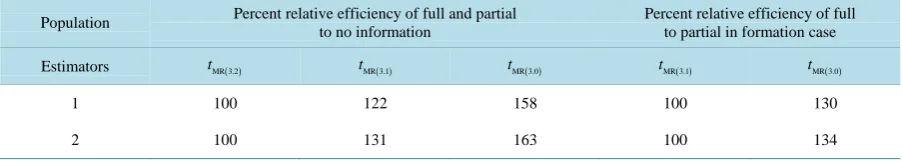
Finally,Table 2 compares the efficiency of full information case and partial case to no information case and full to partial information case. It is observed that the full information case and partial information case are more efficient than no information case because they have higher percent relative efficiency than no information case. In addition, the full information case is more efficient than the partial information case because it has a higher percent relative efficiency than partial information case.

5. Conclusions

The percent relative efficiency is used in sample survey to compare the efficiency of different estimators. The estimator with the highest percent relative efficiency with respect to mean per unit is normally considered to be more efficient compared to the other estimators.

According to Table 1, the proposed Mixture Regression estimators using multiple auxiliary variables and attributes in two-phase sampling has the highest percent relative efficiency compared to mean per unit, Regres-sion estimators using one auxiliary variable and attributes, RegresRegres-sion estimators using multiple auxiliary va-riables and attributes. This means that the ratio-cum-product estimator in two-phase sampling is the most effi-cient estimator compared to the estimators that utilize auxiliary variables and attributes.

The Mixture Regression estimators were then extended to two-phase sampling in partial and no information case. InTable 2, we compared theefficiency of full and partial information case to no information case and

Table 1. Relative efficiency of suggested estimator with respect to mean per unit estimator for two phase sampling.

Estimators

Relative efficiency of suggested estimator with respect to mean per unit estimator

for two phase sampling

Population I Population II

2

y 100 100

REX

t 135 140

REP

t 127 130

MREX

t 199 183

MREP

t 183 175

( )

MR 3.0

t (proposed) 211 274

Table 2. Comparisons of full, partial and no information cases for proposed mixture regression estimator.

Population Percent relative efficiency of full and partial to no information

Percent relative efficiency of full to partial in formation case

Estimators tMR 3.2( ) tMR 3.1( ) tMR 3.0( ) tMR 3.1( ) tMR 3.0( )

1 100 122 158 100 130

(12)

found that the two are more efficient than the no information case. We also compared the efficiency of full in-formation case to partial inin-formation case and found that the full inin-formation case is more efficient than the par-tial information case.

The proposed Mixture Regression estimator using multiple auxiliary variables and attributes in two-phase samplingis recommended to estimate the finite populations mean for full information case as it outperforms all the other existing estimators for full information using one auxiliary or multiple auxiliary variables and attributes. It also outperforms Mixture Regression estimators using multiple auxiliary variables and attributes in partial and no information cases.

When some auxiliary variables are unknown, the two-phase sampling is recommended. If some auxiliary va-riables are known, the Mixture Regression estimators using multiple auxiliary vava-riables and attributes in partial information case should be used but if all the auxiliary variables and attributes are unknown. Mixture Regression estimators using multiple auxiliary variables in no information case should be used to estimate the finite popula-tion mean.

References

[1] Neyman, J. (1938) Contribution to the Theory of Sampling Human Populations.Journal of the American Statistical Association, 33, 101-116. http://dx.doi.org/10.1080/01621459.1938.10503378

[2] Hansen, M.H. and Hurwitz, W.N. (1943) On the Theory of Sampling from Finite Populations. Annals of Mathematical Statistics, 14, 333-362. http://dx.doi.org/10.1214/aoms/1177731356

[3] Cochran, W.G. (1940) The Estimation of the Yields of the Cereal Experiments by Sampling for the Ratio of Grain to Total Produce. Journal of Agricultural Science, 30, 262-275. http://dx.doi.org/10.1017/S0021859600048012

[4] Watson, D.J. (1937) The Estimation of Leaf Areas. Journal of Agricultural Science, 27, 474. http://dx.doi.org/10.1017/S002185960005173X

[5] Olikin, I. (1958) Multivariate Ratio Estimation for Finite Population. Biometrika, 45, 154-165. http://dx.doi.org/10.1093/biomet/45.1-2.154

[6] Raj, D. (1965) On a Method of Using Multi-Auxiliary Information in Sample Surveys. Journals of the American Sta-tistical Association, 60, 154-165. http://dx.doi.org/10.1080/01621459.1965.10480789

[7] Robson, D.S. (1952) Multiple Sampling of Attributes. Journal of the American Statistical Association, 47, 203-215. http://dx.doi.org/10.1080/01621459.1952.10501164

[8] Zahoor, A., Muhhamad, H. and Munir, A. (2009) Generalized Multivariate Ratio Estimator Using Multiple Auxiliary Variables for Multi-Phase Sampling. Pakistan Journal of Statistic, 26, 569-583.

[9] Zahoor, A., Muhhamad, H. and Munir, A. (2009) Generalized Regression-Cum-Ratio Estimators for Two Phase Sam-pling Using Multiple Auxiliary Variables. Pakistan Journal of Statistics, 25, 93-106.

[10] Simiuddin, M. and Hanif, M. (2007) Estimation of Population Mean in Single and Two Phase Sampling with or with-out Additional Information. Pakistan Journal of Statistics, 23, 99-118.

[11] Jhajj, H.S., Sharma, M.K. and Grover, L.K. (2006) A Family of Estimator of Population Mean Using Information on Auxiliary Attributes. Pakistan Journal of Statistics, 22, 43-50.

[12] Naik, V.D. and Gupta, P.C. (1996) A Note on Estimation of Mean with Known Population of Auxiliary Character. Journal of the Indian Society of Agricultural Statistics, 48, 151-158.

[13] Rajesh, S., Pankaj, C., Nirmala, S. and Florentins, S. (2007) Ratio-Product Type Exponential Estimator for Estimating Finite Population Mean Using Information on Auxiliary Attributes. Renaissance High Press, USA.

[14] Bahl, S. and Tuteja, R.K. (1991) Ratio and Product Type Estimator. Information and Optimization Science, 12, 159- 163. http://dx.doi.org/10.1080/02522667.1991.10699058

[15] Hanif, M., Haq, I.U. and Shahbaz, M.Q. (2009) On a New Family of Estimator Using Multiple Auxiliary Attributes. World Applied Science Journal, 11,1419-1422.

[16] Moeen, M., Shahbaz, Q. and HanIf, M. (2012) Mixture Ratio and Regression Estimators Using Multi-Auxiliary Varia-ble and Attributes in Single Phase Sampling. World Applied Sciences Journal, 18, 1518-1526.

[17] Kung’u, J. and Odongo, L. (2014) Ratio-Cum-Product Estimator Using Multiple Auxiliary Attributes in Single Phase Sampling. Open Journal of Statistics, 4, 239-245. http://dx.doi.org/10.4236/ojs.2014.44023

[18] Kung’u, J. and Odongo, L. (2014) Ratio-Cum-Product Estimator Using Multiple Auxiliary Attributes in Two-Phase Sampling. Open Journal of Statistics, 4, 246-257. http://dx.doi.org/10.4236/ojs.2014.44024

(13)