Electrode Kinetic Studies Using a Computerized Data Acquisition and Analysis System

Thesis by Roger Henry Abel

In Partial Fulfillment of the Requirements For the Degree of

Doctor of Philosophy

California Institute of Technology Pasadena, California

1971

Acknowledgments

I am indebted to my research adviser, Dr. Fred Anson, for helping to make my graduate study a rewarding and stimulating experience. I wish to acknowledge the invaluable assistance and suggestions that he has given me and the untiring patience he has shown toward me. I wish to also acknowledge the aid and friendship I have received from Dr. George Lauer, Dr. Donald Barclay, Hong Sup Lim and the other members of Dr. Anson's research group.

I wish also to acknowledge the financial aid that has been provided for me by the Institute and by the Danforth Foundation and National Science Foundation in the form of predoctoral fellowships.

Abstract

The first section of this dissertation introduces the basic concepts that are necessary for the quantitative description of electrode kinetics. The refinements and corrections in the rate equation that are due to a detailed model of the electrical double layer, and to the potential step relaxation technique are introduced and discussed.

A discussion of the non-linear statistical analysis techniques that are necessary for a rigorous analysis of rate equation is

presented in the second section. The estimates of the precision of the desired parameters obtained by using statistical methods can be used as a measure of the efficiency of an experiment. Their use as measures of "kinetic information density" is developed and illus-trated by comparing charge and current measurement in the potential step technique. Previous approaches to the subject of nkinetic

information density" are discussed and compared to the results from statistical analysis.

The third section describes the computerized data acquisition and analysis system that was designed and used for the study of electrode kinetics.

The final section presents the results of the kinetic studies undertaken on the Zn +z /Zn(Hg) system in 1 F NaN0₃, 1 F NaClO ₄, and 1 F NaCl supporting electrolytes. Ensemble averaging is used

- J

The results that are obtained for the rate constants in the various supporting electrolytes are compared and it is shown that the rates are comparable in NaN0₃ and NaC10₄ supporting electro-lytes but significantly greater in 1 F NaCl. These results are compared with results of previous investigators and the quality of the results of this thesis are compared to those of previous

TABLE OF CONTENTS

Acknowledgments Abstract

I. Electrode Kinetics: Introduction and Development of the Rate Equation

Introduction to Electrode Kinetics Basic Theory of Electrode Kinetics

The Double Layer and Electrode Kinetics The Potential Step Method, Mass Transfer

Considerations

H. Utilization of Statistical Techniques in Electrode Kinetics Experiments

Statistical Analysis of Kinetic Data

Statistics and Kinetic Information Density III. Acquisition and Analysis of Kinetic Data by a

Digital Computer

IV. Investigation of the Zn +2 /Zn(Hg) Electrode Reaction in 1 F NaN0_{3 ,} 1 F NaC10_4, and 1 F NaCl

References

Appendix A

Appendix B

Propositions

100 104

108

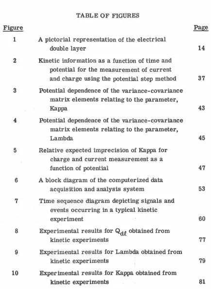
TABLE OF FIGURES

Figure Page

1

A pictorial representation of the electrical

double layer

14

2 Kinetic information as a function of time and potential for the measurement of current

and charge using the potential step method

37

3 Potential dependence of the variance-covariance

matrix elements relating to the parameter,

Kappa

43

4 Potential dependence of the variance-covariance matrix elements relating to the parameter,

Lambda

45

5 Relative expected imprecision of Kappa for charge and current measurement as a

function of potential

47

6 A block diagram of the computerized data

acquisition and analysis system

53

7

Time sequence diagram depicting signals and

events occurring in a typical kinetic

experiment 60

8 Experimental results for Qd£ obtained from

kinetic experiments

77

9 Experimental results for Lambda obtained from

kinetic experiments

79

10

Experimental results for Kappa obtained from

[image:7.617.116.551.84.679.2]

I. Electrode Kinetics: Introduction and Development of

Introduction to Electrode Kinetics

Charge transfer reactions occurring between an electrode and a chemical species in solution are heterogeneous reactions. The rates of these reactions are profoundly affected by the conditions in the region of the solution-electrode interface. This type of reaction has been of interest for some time and several books and articles are available which deal with both theoretical and practical aspects of this subject (1-9).

When relaxation methods are used to study the kinetics of charge transfer reactions, not only must one take into account the state of the interfacial region but also the rate and means of transport of the

reacting species to the reaction site (the electrode) must be considered. By choosing ·appropriate experimental conditions, e.g., a large excess of indifferent ions and relatively short experimental times, transfer of the reacting species to the electrode by migration and convection can be neglected. Transfer of the reacting species then takes place solely by diffusion, usually linear and semi-infinite. As long as the rate of the charge transfer reaction is controlled primarily by the kinetics of the charge transfer, information can be obtained about these kinetics, but when the rate of the charge transfer reaction becomes limited by the rate at which reacting species can diffuse from the solution to the · electrode no information can be gained about the kinetics of the actual

reacting species is uniform throughout the solution. After the experi-ment is initiated, it is often possible to assume that the initial uniform concentration is maintained for short times. However, after the

reaction has proceeded sufficiently, the reacting species will become depleted at the electrode and a concentration gradient will be set up which will cause reactant in the solution to diffuse to the electrode. Thus the rate of the reaction is controlled primarily by the rate of the charge transfer process at short times, while at longer times,

diffusion becomes more and more important and eventually the rate of the reaction will be determined entirely by the rate of diffusion of the reacting species to the electrode. One can discuss three time ranges in an experiment. In the first, the rate of the reaction is controlled by the rate of charge transfer, in the second there is mixed control by diffusion and charge transfer, and in the third range the rate of the reaction is controlled by the rate of diffusion of the reacting species.

In the past, it has been commonplace to attempt to obtain all of the data in the first-time range so that the effects of diffusion can be neglected and a simplified model employed' in analysis of the data. However, conditions where the simplified analysis can be made prove to be very restrictive in terms of the time range that is avail-able and the magnitude of the charge transfer rates that can be

reactions are partially controlled by diffusion even at the shortest times that are available to the experimenter and for these reactions the effect of diffusion on the overall rate must be taken into account to obtain valid estimates of the rate of charge transfer. The equations which are applicable to this situation are nonlinear in the parameters which are to be determined and thus linear least-squares analysis techniques of the types generally employed cannot be used. Previous workers have generally avoided the rigorous analysis and have used

I

instead simplified, approximate models for the more complex rigorous equations. While this approach does make possible the study of rates of charge transfer that are faster than can be accom-modated w~th the first approach, it still leads to quite restrictive experimental conditions. In addition, there is a real danger that the approximate equations will be applied under circumstances where they are not applicable (10). The use of simplified approximations was well justified when analysis of the data was undertaken using

manual or desk computation, however because of the ready availability of computers today~ the rigorous equations~ even though they a:re non-linear, do not present a major problem for analysis.

no more information about the rate of the charge transfer process is obtainable. The point in time at which this change from partial control to full control by the rate of diffusion takes place is not well defined, rather it is a gradual change and is largely determined by the accuracy and precision with which one can obtain the data. That is, the more precise the data that are obtained, the higher the rate of charge transfer one can measure before one must consider the

reaction to be diffusion controlled. Even a computerized data analysis will not yield improved results unless the data being analyzed are sufficiently accurate and precise.

In order to optimize the experimental situation, we set out to develop a computerized system which could control the experiment, obtain highly precise data, and analyze the data using a rigorous

this divergence in the results and the resulting uncertainty in the absolute values of the rates, conclusions that are drawn concerning small variations in the rate constant that occur in different supporting electrolytes, or at different temperatures, etc. are not very convinc-ing. Even though there is a lack of reproducibility of results that have been reported, several investigators have reported that the rate

constant for the reduction of zinc varies with supporting electrolyte used (14-18). The rate of the reaction appears to become greater when chloride is substituted for nitrate or perchlorate and the enhance-ment of the rate when bromide is used appears to be even greater than with chloride. The reduction of zinc in various supporting electrolytes .was chosen for study because this reaction displays a rate that is in a

Basic Theory of Electrode Kinetics

Before discussing the experiments and results in detail, some of the basic ideas of electrode kinetics will be presented and applied to the particular relaxation technique that was used in these investi-gations. The aim in presenting these basic ideas on electrode kinet-ics is not to be exhaustive but rather to provide those concepts which are necessary for latter discussions. For a more thorough develop-ment of these ideas the reader is referred to Delahay's, "Double Layer and Electrode Kinetics" (2).

In this presentation we will make several assumptions which will be mentioned before proceeding further. Because the activities of the species in solution are generally not available, their activities will be approximated by concentrations. If the activities do happen to be known the resulting equations in concentration terms can be simply corrected. Another assumption that we will make initially is that the reacting species can reach the electrode as fast as necessary to maintain a uniform concentration throughout the solution, i.e., the rate of diffusion will be assumed to be very fast compared to the rate of electron transfer. This assumption enables us to neglect the

mass-transfer process and concentrate on a description of the

and develop kinetic equations which are general and independent of the

technique chosen to study the kinetics. The reaction to be described

(Eq. (1)) is assumed to be first order in. the reacting species and it is

assumed that the number of electrons transferred in the overall

:reaction (n) are transferred during the rate-determining step.

z

Ox + ne (1)

where Oxzis the oxidized species with a charge of z, Red is the

reduced species which has a charge of (z-n), and n is the number of electrons involved in the charge transfer reaction. Reaction (1) is a first-order heterogeneous reaction, the rate of which is expressed in .

units of moles/cm2 _{/sec. The heterogeneous rate constants, kf and}

kr, have units of cm/sec.

d[Ox~ d[Red (z-n)]

Rate

= =

dt dt

= ~[oxZ] - k _r [Red(z-n)] (2)

The rate is more conveniently expressed and measured in terms

of current density~ i, obtained by multiplication of the rate by the number of electrical equivalents per mole:

i = n F (Rate) (3)

constant. Reduction current is taken as positive and oxidation current negative (2). The rate constants, kf and kr, will differ from ordinary chemical rate constants because they will be strongly influenced by the electrical field that is present at the electrode-solution interface, i.e., they will depend on the electrode potential.

The theoretical equations that describe the rate process occur-ringat the electrode can be developed analogously to the

non-electro-chemical case with the exception that the standard free energy of activation becomes a standard electrochemical free energy of activa-tion, which is dependent on the potential difference at the electrode solution interface. The standard electrochemical free energy of activation, AG0

*,

is described by the following equation (19)

AG0_c

*

+ anFE (4)

where

AG~*

is the standard chemical free energy of activation and a is a number having a value between zero and one. This fraction, a, is called the symmetry factor (20), and the term an FE is the fraction of the electrical energy n FE where E is the potential differ-ence between electrode and solution that contributes to the standard free energy of activation for the forward reaction (reduction).

Similarly, (1 - a)nFE measures this contribution in the reverse direction (oxidation).

ka, may be defined which are independent of the potential. The rate

expression then becomes:

where [Ox] and [Red] are the concentrations of the oxidized and

reduced species at the reaction sites and E is the potential of the

electrode versus some reference electrode. The rate constants

defined in this way depend on the particular reference electrode used,

and it is more meaningful to derive expressions for rate constants

which are independent of the particular reference electrode used.

To do this, we must consider the system under equilibrium conditions

with both reactants in their standard states. Under these conditions,

there is no net current and the potential at the electrode interface is

the standard potential, E0 , for the particular redox couple under

consideration.

Since there is no net current and since both 0 and Red are in

their standard states Eq. (5) may be written:

i

=

O

=

nF{ k exp[-anF E0 _{] - k exp[(l-a)nF E}0

J)

₍₆₎

c RT a RT

k exp[- a:nF E0

] = k exp[ (l-a)nF E0 ]

=

ka (6a)

c RT a RT s

By using the above definition for the apparent standard rate

follows:

i = nFk:[ [Ox] exp{ -

~U:

(E - E0) }

- [Red] exp{ (1-a)nF (E - Eo)}]

RT

(7)

the form of Eq. (7) is now independent of the particular reference electrode used as is the value of the rate constant,

k;,

since it

refers to the standard potential where forward and reverse rates are

I

equal under standard conditions. The va1Je of

k:

is thus truly characteristic of the particular electrode reaction.

Equation (7) is the basic equation that is used to describe a charge transfer reaction; however there are two additional corrections that must be made in the rate equation, which incidentally is the

The Double Layer and Electrode Kinetics

The model that is currently used to describe the electrical

double layer which exists at the surface of the electrode was developed

independently by Gouy (21) and Chapman (22) and later modified by

Stern (23). In the interfacial region at the electrode surface there

are solvent molecules and ionic species and since the potential at the

metal electrode is in general different from the potential in the bulk

of the solution the charged species in solution are either attracted to

or repelled from the electrode by the electrical field which exists.

Reactants are assumed to be able to approach the electrode surface

up to a certain distance which is of the order of the radius of a

solvated ion (Fig. 1). This plane of closest approach for solvated

ions, at a distance of

x

₂ from the electrode surface, is called the

outer Helmholtz plane. Under some conditions, certain ions will

lose their associated solvent molecules in the direction of the

elec-trode and approach to a plane situated at a distance of X1 away from

the electrode surface. This plane is called the inner Helmholtz plane

and the ions which are located at this plane are described as

specifi-cally adsorbed. The potential in the double layer region referred to

the potential in the bulk of the solution will vary with distance from

the electrode and at a distance X from the electrode the potential will

be </>. Then by introducing a Boltzmann distribution function the

concentration of ionic species in the double layer region can be

Figure 1. A pictorial representation of the interfacial

Electrode Surface

Potential

~ X1 inner Helmholtz plane

I I

1 :~ x2 outer Helmholtz plane I I

I I

I I I I

,a

( b) Ions with solvotion shell

{a). Specifically adsorbed ions

Distance from electrode

Diffuse double.

layer

....

Frumkin (24) was the first to correlate this picture of the double layer with electrode kinetics and demonstrate the expected effects of the double layer conditions on electrode kinetics. He assumed that the electron transfer reactioh takes place with the reactants at the outer Helmholtz plane. Therefore two corrections must be made to the Eq. (7) describing the charge transfer reaction. The concentration of charged species at the outer Helmholtz plane will in general be different from their bulk concentrations and will be

given by

(Ba)

and also the effective potential, the potential at the outer Helmholtz plane is

Thus, the corrected kinetic express ion then becomes

{ amF ( o } exp - - - E - </>_{2 -} E )

RT

(Z - n - Z )F (l ) }

- (Red) B exp ox RT R </>2 exp -:TnF (E - Eo) . (10)

Furthermore, if Z₀x = ZR + n this expression becomes

(11)

a

If the apparent standard rate constant, ks , is defined in the following

way,

Eq. (7) and Eq. (11) are identical.

Since the necessary double layer data are often unavailable,

the most frequently reported rate constants are actually only apparent

rate constants, uncorrected for double layer contribution.

The potential, _</>2, in Eq. (12) is the potential at the outer

Helmholtz plane when the electrode potentrl is that at which the rate

constant is being measured. Since </>₂ is a function of the electrode

potential9 the apparent rate constants obtained from kinetic

experi-ments will also be potential dependent. If, in addition, the variation

potential ranges, a Tafel plot (2), 1.n i vs. (E - E0), will yield values of the transfer coefficient, obtained from the slope, which differ from the real transfer coefficient.

If double layer data are available, the standard, potential-independent rate constant as well as the true tr an sf er coefficient can be obtained. Equation (11) can be rearranged into the following form,

( Z0x F ) i exp RT ¢2

= [Ox] nFk exp-amF (E-cp -E0 )

. B s RT 2 ( 1 - [Red] B exp[ nF (E - E0) ] )

[Ox]B RT

(lla) Now a plot of the logarithm of the left-hand side of Eq. (lla) against (E - </J_{2 -} E0) will have an intercept proportional to the standard

,•

The Potential Step Method. Mass Transfer Considerations The particular form of the kinetic equations that result when mass transfer effects are included vary with the relaxation technique that is used for the kinetic investigation. We will consider the

potential step method (4₁ 25) applied under conditions where convection and migration effects can be ignored so that semi-infinite linear

diffusion is the single operative mass transport process. The

measured response is either current or its integral, charge. Since we will be assessing the relative merits of charge and current

measurement, equations for each case will be given.

In this technique, the potential of the electrode at which the kinetics are to be measured is controlled by a potentiostat which can abruptly change the potential of the electrode and maintain it at any value by supplying the necessary current. Initially 1 the electrode, a

hanging mercury drop of known area immersed in a solution contain-ing only the oxidized half of the redox couple to be studied, is main-tained at a potential such that no reaction occurs. The

potential of this electrode is then stepped to a value where the charge transfer reaction occurs. Information about the electron transfer rate is obtained by analyzing the resulting time transient of either the current or charge.

A. Current as a function of time (25)

2 .!

i(t)

=

K exp(X t) erfc(Xt 2) + id

1(t) (13)

B. Charge as a function of time (26)

[

1 .!.

J

Q(t) =

...!£

exp{X2_{t) erfc(xtz) +} 2

~ta

_{- 1}

~2

-I\. 7T2

+ Qdl (14)

where

[

exp(-w(E-E0)]

exp[(l-~~nF

(E-E0)]

J

X = ka + (16)

s

D 1/2 D 112

. ox R

erfc(y)

- - J

2 00 e -t dt (2 7) 2 1/2 .

1T y

In the above equations i(t) and Q(t) are the total current and

charge at a time,

t,

id₁(t) and Qd.e_(t) are the current and charge at

any time,

t,

involved in the charging of the electrical double layer

existing at the electrode, A is the electrode area, and D₀x and DR

are the diffusion coefficients of the oxidized and reduced species.

Kappa, K, is the current that would flow if mass transfer of the

reactants were very high and is a measure of the intrinsic electron

of mass transfer on current. This function varies from a value of

one when its argument is zero to a value of zero when the argument,

y, becomes large. When y

=

5, the function has a value of 0. 1107.

1

Since y

=

A.t2 , mass transfer effects become more significant as

Lambda, A, or time become large. Lambda becomes larger as the

apparent standard rate constant,

k:,

becomes larger, as the absolute

value of (E - E0) becomes larger, or as the diffusion coefficients,

D

0x and DR, become smaller. Simply stated, this means that

when-ever the prevailing rate of electron transfer is sufficiently rapid

compared to the rate of diffusion of the reacting species its

concen-tration at the electrode surface will become depleted and the overall

rate of the reaction will become controlled by the rate of mass

II. Utilization of Statistical Techniques in Electrode

Statistical Analysis of Kinetic Data

The theoretical equations for the time response of either current or charge (Eqs. (13) and (14)) are non-linear in the parame-ters to be determined, Kappa, Lambda, and the double layer charging, id1(t) or Qd1(t). Successive approximation methods must be used to obtain the desired kinetic parameter. The three general methods that are most often employed are linearization using a Taylor series expansion, steepest descent, and Marquardt's compromise (28). For the experiments that were carried out in this research, lineari-zation by Taylor series expansion was chosen and employed. This method has the disadvantage that there is a danger of divergence if the initial estimates for· the parameters are too far removed from the final optimal estimates. Fortunately, it was generally possible to obtain sufficiently good initial estimates in the cases studied. The advantage of this method over the alternate methods is that when it does converge it generally converges more rapidly. In addition, this method is less complex mathematically than the others.

The Taylor series expansion method (28, 29) will be illustrated using the equation for the charge measurement variation of the

potential step technique. We will assume that the double layer has been charged by the time at which the first measurement is taken so that the charging term may be treated as a constant parameter

with only slight modification.

The equation for the charge time response can be written in the

following form:

Q(t)

=

a + Gf(ct) + e (17)

where Q(t) is the measured charge at anytime; a, b, c are the

param-eters to be determined and the best estimates for them are given by

a,

b, C;

and E is the error associated With the measurement Of the

charge. If the initial estimates for the parameters are sufficiently

close to the final estimates, the equation can be expanded using a

Taylor series expansion neglecting terms that are higher than first

order. If the initial estimates for the parameters are a0 , b0 , c0 _and

the final estimates are

a,

b,

c

and we let

Q

=

Q(a,

s~

c,

t)

then

if we define

Q-Qo

=

y

y ~

6

p. z!> + E.

i 1 1 (18)

Equation (18) is now in a linear form which is suitable for linear least-squares analysis. The normal equations resulting from this analysis can now be solved for the parameters, pi, which are to be estimated. These estimations, pi, can be combined with the initial estimates, a0

, b0, c0, to provide improved initial values for another

Taylor series expansion. This iterative process is continued until the estimates have converged to the desireid degree. Equation (18)

i

was written for one experime.ntal point but in general the experiment consists of n experimental points which are to be analyzed to provide the best estimates for the parameters. For the general case we can write·, using the preceding definitions,

0 0 0 Z11 Z21 Z31

z

=

0 0 0

Z12 Z22 Z32 p = Pz

where Z, Y, and Pare matrices

The solution for P, the parameter estimates, is given by

P

=

(Z'Zf1

z'y

(19)

the form of the above equation is the same as in the linear case since

a linear approximation for the theoretical non-linear equation was

used.

The most significant difference is that the independent variable

matrix, Z, is a function of the parameters in the non-linear case

while with a linear equation the matrix is independent of the

parame-ters which are to be estimated and is a function only of the independent

variables. In the linear case when it can be assumed that the variance

can be associated with the dependent variables or at least that the

variance associated with the dependent variable is very much larger

than any variance associated with the independent variables, estimates

for the variance associated with the estimated parameters are given

by the following equation

Var(p·) ₁

=

v .. ₁₁ a2 (20)

where

cl

is the variance associated with the dependent variable and

vii are the diagonal elements of the variance-covariance matrix,

(Z'

Zf

1• In the linear case the diagonal elements

vii

of the

variance-covariance matrix are functions only of the independent

variable and can be thought of as scale factors which relate the

parameters. Because the variance-covariance matrix in the non-linear case is a function of the parameters to be estimated it will have some variance associated with it as distinguished from the linear case. Thus the estimates obtained for the variance of the parameters estimated will only be approximate and will be lower limits. How-ever, except in cases of extreme non-linearity, the estimates arrived at for the variances of the determined parameters will be good (30).

If we return to the linear case, another use of the variance-covariance matrix can be pointed out. As was stated, the diagonal elements of this matrix can be considered as a set of scale factors which relate the variance of the dependent variable to that of the

estimated parameters. These scale factors can be varied by choosing different ranges for the independent variables and thus the estimates for the variance of the parameters can be varied. To relate this to a specific example, if we were to determine the slope of a straight line by sampling at various points along this line, we would expect to be able to determine the slope with more precision with the samples well spaced along the line than if the samples were clustered about one point. For the same variance associated with the dependent variable? the scale factors would be higher for the clustered points than for the well-spaced points so the variance estimates of the slope would be higher in the case with the clustered points. These scale factors~ the diagonal elements of the variance-covariance matrix, give an indication of the efficiency of our experimental design.

of the dependent variable, the smaller the estimated variance of the

parameters, or, in other words, the greater the information which

we have obtained from the given experiment. The reciprocals of the

scale factors are thus proportional to the amount of information which

we have obtained by using a given experimental design. In choosing

a particular experimental design we would like to maximize the

information which we can obtain about the parameters or, equivalently,

minimize the variance of these parameters.

If we return again to the non-linear case, the previous discussion

I

is only approximately true because the scale factors are not

indepen-dent of the parameters estimated. However the diagonal elements of

the variance-covariance matrix will give lower limits in estimating

the parameter variance and their reciprocals will give upper limits in

estimating the information derived about the parameters. Examination

of the diagonal elements of the variance-covariance matrix for several

experimental designs will enable the experimenter to choose the

particular design which will serve to maximize the information about

the parameters in which he is interested. This type of approach also

enables the experimenter to choose between several experimental

techniques, each of which may provide estimates for the parameters

Statistics and "Kinetic Information Density"

There has been some discussion (10, 31-33) previously in the

literature about the relative merits of current or charge

measure-ment techniques to gain information about electrode kinetic

parame-ters. Various approaches have been taken in the past to try to

esta-blish the relative advantages of each method. These previous

analy-ses have reached varying conclusions depending upon the criteria of

quality employed. We decided to address the problem by comparing

the expected variance of the estimated parameters arising from the

two techniques to assess their relative merits.

Before discussing the results of these comparisons the past

approaches that have been used and their shortcomings will be pointed

out.

It has been asserted (32, 34) that the measurement of charge

should be superior to the measurement of current because charge,

being the integral of the current retains information about the kinetics

of reactions which occurred at all earlier times during the integration.

While this is an appealing intuitive argument it would be more

power-ful and compelling if it could be put in more quantitative terms.

In an attempt to do this Oldham and Osteryoung (10) and, more

recently, Osteryoung and Osteryoung (33) have put forward the

following ideas: the net response (current or charge) can be thought

of as a combined response due to both mass transfer, which is

the rate process of interest. The amount by which the kinetics of charge transfer diminishes the measured response compared to the response that would result from pure diffusion control is a direct measure of the "kinetic information" contained in the response and is called the "kinetic information density". These authors have com-pared the kinetic information density of charge and current measure-ment and have concluded that under the usually accessible experi-mental conditions charge measurement is superior to current

measurement. This definition allows the ''kinetic information densi-ty" to be quantified but there are still some shortcomings to this approach: An ideal, errorless experiment is considered rather than a more realistic experimental situation. The approach taken by Osteryoung and Osteryoung neglects the problem of a realistic appraisal of experimental error. An experiment where current or charge could be measured without error would~ by their definition, have the same "kinetic information density" as an experiment where there was a great deal of error in measuring current or charge.

Their approach gives the "kinetic informatiOn density" of the response for a particular combination of the kinetic parameters and the inde-pendent variable while in a actual experiment one obtains and analyzes data for a range of values of the independent variable and the "infor-mation density" for that particular experimental design is of more

immediate use and importance than the "information density" at one

particular point in the experiment. It is also reasonable to expect

kinetic information would be different than the sum of the kinetic

information density at each of the data points.

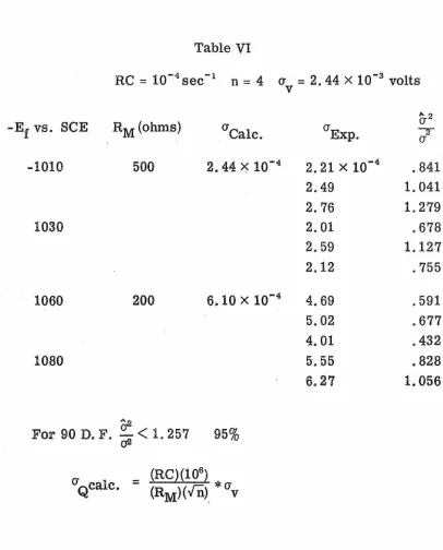
What follows is an error analysis for the two techniques under

consideration. This analysis employs standard, well-known methods

(30, 35-37) which, however, have not been directly applied to

measure-ments of electrode kinetics. One is interested in assessing the errors

to be expected in the kinetic parameters to be evaluated, arising from

the unavoidable errors in the experimental measurement of charge or

current. Equation (20) gives the relationship between the variance of

the measured response and expected variance of the parameters. In

comparing two techniques which estimate the same parameter, the

technique which gives the more precise estimate for the parameter is

the better technique. If the two techniques have the equal values for

the variance of the measured response,

(i,

then the technique which

has the smaller diagonal element that relates the variance of the

measured response to the variance of the parameter is the better

technique.

Since Kappa is the kinetic parameter that is used to determine

the standard rate constant a comparison of the estimated variance of

Kappa for charge and current measurement will give an indication of

the relative merits of the two techniques. Using Eq. (20)

(21a)

or Var (KQ) _ vQ

aQ

Var (KI) - VI

a;

(22)

where Var(KQ) and Var(KI) are the estimated variances of the

param-eter Kappa when charge and current are measured, vQ and vI are the

corresponding diagonal elements of the variltnce-covariance matrix

and

aQ

and

al

are the variances of the measured variable, charge

and current. The reciprocals of the estimated parameter variances

will be proportional to the information obtained by the particular

experiment so Eq. (22) can be rewritten:

(23)

where Inf(KQ) and Inf(KI) are measurements of the amount of

infor-mation about the parameter Kappa that are obtained when measuring

charge and current.

To make explicit comparisons between charge and current

measurement, the experimental design must be specified. Also since

the equations are non-linear particular values for the parameters to

be determined must be specified. The values of the parameters and

constants chosen for this analysis were selected because they match

the corresponding parameters for the electrode reaction that was to

be studiedj zn+2 _{/Zn(Hg). Inasmuch as the standard rate constant and}

the time were varied over wide ranges, the particular values that

affect the results but they will not affect the trends that are apparent

in the results nor the conclusions that will be drawn. The diffusion

coefficients of the oxidized and reduqed species were set equal to

9 x 10-6 _moles/cm3

, and the following constants were assigned values as follows:

n = 2

A = .032 cm2

C = 1 x 10-6 moles/ cm3

a

=

O. 2

Calculations were made for the standard rate constant equal to

1 x 10-3

, 1 x 10-2, and 1 x 10-1 cm/sec. Comparisons were made for experimental designs where the first data point would be taken at times

ranging from 10 µseconds to 0. 1 seconds. The experimental design analyzed assumed fifty equally spaced data points for each comparison

I

and the spacing between data points was made equal to time between

the initiation of the experiment and the first-data point. That is, if

the first-data point was to be taken at 10 µseconds after initiation of the experiment then 50 data points would be taken having a interval

between each other of 10 µsec. Correspondingly, if 0.1 second was to be the time of the first-data point then the sampling interval was

chosen to be 0. 1 second. The potential was varied to include values of

~~

(E - E0) of

O~

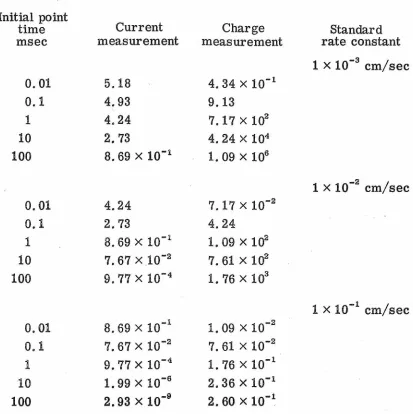
-1, and -2 corresponding to potential steps of O,

[image:40.612.129.542.142.556.2]

Table I. Information (Kappa)

Initial point

Current Charge

time Standard

msec measurement measurement rate constant

1 x 10-3 cm/sec

0.01 5.18 4. 34 x 10-1

0.1 4.93 9.13

\

1 4.24 7.17Xl02

10 2. 73 4. 24 x 104

100 8. 69 x 10-1

1. 09 x 106

1 x 10-2 cm/sec 0.01 4.24 7. 17 x 10-2

0.1 2.73 4.24

1 8. 69 x 10-1 1. 09 x 102 10 7. 67x10-2 7. 61 x 102 100 9. 77 x 10-4 _1.

76 x 103

1 x 10-1 cm/sec 0.01 8. 69 x 10-1 1. 09 x 10-2

0.1

7. 67 x 10-2 7. 61x10-2 1 9. 77 x 10-4 _1.

lnitial point time msec 0.01 0.1 1 10 100 0.01

0.1

1 10 100 0.01 0.1 1

10

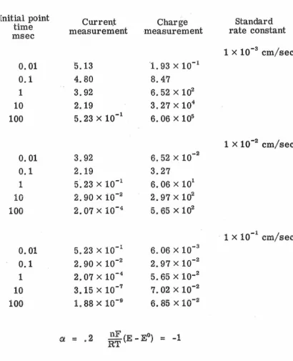
100

Table II. Information (Kappa)

Current Charge

measurement measurement

5.13 1. 93 x 10-1

4.80 8.47

3.92 6. 52 x 102 2.19 3. 27 x 104 5. 23 x 10-1 6. 06 x 105

3.92 6. 52 x 10-2

2.19 3.27

5. 23 x 10-1 6. 06 x 101 2. 90 x 10-2

2.97X102 2. 07 x 10-4 _{5. 65 x 10}2

5. 23 x 10-1 6. 06 x 10-3 2. 90 x 10-2 2. 97 x 10-2 2. 07 x 10-4 _{5. 65 x 10-}2 3. 15 x 10-7 7. 02 x 10-2 1. 88 X 10-G 6. 85 x 10-2

i[)l

= •

2 nF (E - Eo) = -1

RT

Standard rate constant 1 x 10-3 cm/sec

1 x 10-2 cm/sec

[image:41.617.131.541.145.650.2]

[image:42.617.127.545.157.650.2]

Initial point time msec 0.01 0.1 1 10 100 0.01 0.1 1 10 100 0.01

0.1

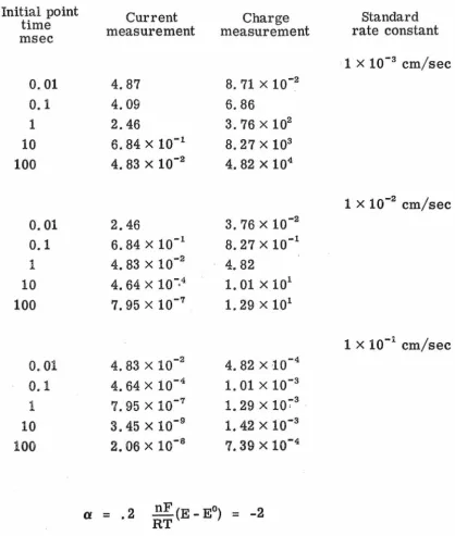
1 10 100

Table III. Information (Kappa)

Current Charge

measurement measurement

4.87 8. 71 x 10-2

4.09 6.86

2.46 3. 76 x 102 6. 84 x 10-1

8. 27 x 103 4. 83 x 10-2

4. 82 x 104

2.46 3. 76 x 10-2 6. 84 x 10-1 8. 27 x 10-1 4. 83 x 10-2 4.82

4. 64 x 10-·4 1. 01 x 101 7. 95 x 10-7 1. 29 x 101

4. 83 x 10-2 4. 82x10-4 4. 64 x 10-4 1. 01 x 10-3 7. 95 x 10-7 1. 29 x 107'3 3. 45 x 10-9 1. 42 x 10-3 2. 06 x 10-s 7. 39 x 10-4

a

= •

2 nF (E - Eo) = -2 RT

Standard rate constant

· 1 x 10-3 _cm/sec

1 x 10-2 cm/sec

Figure 2. Reciprocals of the variance-covariance matrix

diagonal elements relating to the parameter, Kappa,

in kinetic experiments using the potential step

method as functions of time and potential for current

nF

nF

nF

-·

(E-E

0 )

=

0

-(E-E

0 )

=-I

-(E-E

0 )

=

-2

RT RT RT ---Charge Current k k 6 (rate constant) I 1 x 10 -3 (rate constant)/ 1 x 10 -3 5 I /

I

I 4 1 1 -IX 16 2 I 3

I

-2

-,,

I

,,.-Ix 10 >-2

//

-1/

I/

·-

"'

/I I/

~-_I

---IX 10-2 c I G.>

~1x16

3

~1x16

3

0 0

~

=~~~\\'

·~-z

~~\-\IX16

1

t \\"

IX10~

3 E -3 . I X 10 . -2 -I X 10 I

·

a

·

IX 10 ~

...

-4

c

--5

0

-

-Gt-\

r-\

r-\

\ IX 10-2

C1' 0

were assumed to be equal to one and the kinetic information tabulated is equal to the reciprocal of the appropriate element of the variance-covariance matrices for charge and current measurements. If

aQ

and a

1 2

are equal to each other but not equal to one the ratio will still be the same as the ratio of the tabulated values. If

aQ

and

a:

are not equal, then they must be included to form the correct information ratio.

The particular experimental design for the spacing between data points was chosen to contrast with results of Osteryoung and Osteryoung (33). Since Osteryoung and Osteryoung make their

information", than would current measurement at experimental times

equal to or greater than about 100 µseconds. The actual crossover time

varies but is generally in this neighbor hood. Also the higher the

intrinsic charge transfer tate, ks, or the effective charge transfer

rate, reflected in effect of potential on the information, the smaller

the amount of kinetic information available for a given level of

variance of the measured response. Although at short enough

experi-mental times current measurement would appear to be the technique

of choice other considerations enter in which prevent making a clear

cut distinction. At experimental times that are early enough to be in

a region where current measurement would be superior, the

assump-tion that was made about the charging of the double layer being

com-plete by the time the first experimental point was taken may no longer

be valid. Thus, in most typical experimental situations charge

measurement should be superior to current measurement for

evalu-ating kinetic parameters.

Although the same conclusion was reached by Osteryoung and

Osteryoung on the basis of their analysis, the type of analysis

out-lined here reveals more of the major importance of experimental

design on the information that can be obtained from kinetic

experi-ments. The definition of "kinetic information densityn used by

Oste::ryoung and Osteryoung can not account for the factor of

experi-mental design for two :reasons: first of all it does not treat the

measured response and secondly and more importantly their

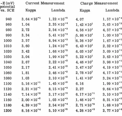
Table IV. Reciprocals of Variance-Covariance Diagonal Elements for Kinetic Parameters for Current Measurement and for Charge Measurement

-E (mV) Current Measurement Charge Measurement potential

vs. SCE Kappa Lambda Kappa Lambda

940 3. 64x10-1 1. 22 x 10-5

4.07 1. 57 x 10-4 960 1. 04 2. 35x10-4 _1. 42 x101 3. 63 x 10-3 980 2.72 2. 54 x10-3 _{4. 56 x10}1 _{4. 57x10-}2 990 3.34 5. 41 x 10-3

15.

86 x 101 1. 00x10-1 1000 3.57 8. 94 x 10-3

6. 36 x101 _{1. 67x10-}1

1010 3.60 1. 24x10-2

6. 43 x 101 2. 32 x 10-1 1020 3.42 1. 66x10-2 _{.6. 03 x10}1 _{3. 09 x 10-}1 1030 3.04 1. 99x10-2 5. 22 x101 _{3. 63x10-}1

1040 2.67 2. 22 x 10-2 4. 46x101 3. 98x10-1 1050 2.17 2. 41 x 10-2 3. 47 x 101 4. 19 x 10-1 1060 1. 81 2. 46 x 10-2 _2.78X101 _{4. 17 x 10-}1 1080 1. 03 2. 10 x 10-2 1.41 x101 3. 24 x10-1

1100 5. 16 x 10-1 1. 45x10-2 6.16 1. 99x10-1 1120 2. 21 x 10-1 _{8.15 x10-}3

2.27 9. 64x10-2

1140 7.14x10-2 _{3. 17x10-}3 _{6. 17 x 10-}1 _{3. 10 x 10-}2

. 1160 2. 00x10-2 1. 03 x10-3

[image:47.612.127.545.182.577.2]

point and therefore is not applicable to the experimental situation as

it is normally encountered.

The previous discussion illustrated the comparison of kinetic

information obtained for a wide variation of time and rate constant.

To provide a more quantitative comparison that reflects more closely

the actual conditions under which the kinetic experiments herein

described were performed, values of the kinetic parameters obtained

from actual kinetic experiments were used to calculate the amount of

kinetic information available from charge and current measurements

under the particular experimental conditions that were employed.

For these experiments one hundred experimental points were used

and a sample was taken every 400 µseconds.

I

Table IV and Figs. 3 and 4 show the reciprocals of the diagonal

elements of the variance-covariance matrices for the kinetic

param-etersy Kappa and Lambda. These results show very strikingly the

effect of potential on the amount of kinetic information that can be

obtained from measurements at various potentials with a given level

of variance of the dependent variable. Figilres 3 and 4 compare charge

measurement versus current measurement and show that charge

measurement should yield superior results over the entire potential

range. Also a comparison of Fig. 3 with Fig. 4 indicates that since

Kappa can be obtained with more precision, i.e. 1 higher information, than

Lambda, it is preferable to obtain the rate constant from Kappa.

Table V and Fig. 5 have been included to indicate more clearly

Figure 3. Potential dependence of the variance-covariance

matrix elements relating to the kinetic parameter,

Information Density Kappa

1''

60

_I

_\

I

\

-

I

\

I

50

_I

_\

I

J...

_I

_\

T

-

c

I

\

Q.) ...

E 40

₄

-Q.)

I

\

c

'- Q.)

::J

I

\

E

en

0 Q)

~

30

3

'-I

_\

::J

en

Q.)

I

\

0

C'i Q.)

'-~

0

.c

₂₀

_I

_\

₂

u

-I

\

c Q)

\

'-i

'-10

::J

Ii

~

u

~

950

1000

1050

1100

1150

1200

Figure 4. Potential dependence of the variance-covariance

matrix elements relating to the kinetic parameter,

Information

Density

Lambda I" ....

I \

.4

I \

I

\

I

_\

I

_\

I

I

\

T

_I

_\

I

I

\

a

.3

.03T

-

-

I

\

c

_I

_\

Q)

E

I

\

-\

-Q)

I

c

"-

_\

_I

())

::>

_I

E

(/)

,

,

0 I

_\

())

())

_I

~

~

.2

_I

\

_\

.02

~

I

a

())

_\

())

~

I

\

~

~

I

0

\

-.r:.

_I

_c

u

_I

\

())

\

~

I

_\ ~ ::>

. I

_I

_\

.01

u

I

_\

I

_\

I

\

I

~

I

I

'

I

'

...

0

~

950

1000

1050

1100

1150

1200

[image:53.615.160.523.175.582.2]

Table V. Logarithm of Variance-Covariance Element of Kappa for Charge and Current Measurement

-E (mV) potential _{Charge Current}

vs. SCE

940 1.221 2.269

960 0.678 1. 813

980 0.170 1. 396

990 0.063 1. 306

1000

o*

1. 256

1010 0.023 1.274

1020 0.050 1. 295

1030 . 0.113 1. 347

1040 0.180 1.403

1050 0.289 1.494

1060 0.386 1. 572

1080 0.681 1. 817

1100 1.040 2.118

1120 1. 473 2.485

1140 2.040 2.976

1160 2.666 3.529

1180 3. 39,7 4.188

1200 4.201 4.916

Figure 5. Relative expected imprecision of Kappa for

charge and current measurement as functions

10,000

c

1,000

0 en

·-

₍₎ Q) !a... 0.

E

Q)

100

>

-

0 Q)

ct:

10

Expected Relative Imprecision Current measurement Charge measurement I

I

I

I

I

I

I

I

I

I

I

I

I

I

I

I

I

I

I

I

\

/'

\

_\

_I

I

\

//

'

'

,,.

_,/

950

1000

1050

1100

-E(mV) vs SCE

table and figure show the increased precision with which it is

neces-sary to measure the dependent variable in order to maintain a

constant level of variance for the kinetic parameter Kappa. The level

of variance for Kappa at -1000 mv vs. S. C. E. for charge

measure-ment was chosen as the desired level. The numbers in Table V are

logarithms of the ratio of variance of the dependent variable at -1000

mv vs. S. C. E. to the variance of the dependent variable at various

other potentials which are necessary to maintain a constant variance

I

for Kappa. Thus for charge measurement~, the charge must be

measured approximately ten times as accurately at -1100 mv vs.

S. C. E. to obtain the same level of variance in Kappa as was obtained

at -1000 mv vs. S. C. E. Likewise the current must be measured

about 18 times more accurately at -1000 mv vs. S. C. E. to obtain

III. Acquisition and Analysis of Kinetic Data by

Computerized Data Acquisition and Analysis System

The components of the computerized data acquisition and

analysis system are shown in a block diagram in Fig. 6. These

components will be described and then the interconnections that are

necessary to provide a useful system for data acquisition and analysis

will be detailed.

The potentiostat used in the experiments is part of a general

purpose electrochemical instrument which: has previously been

described (38). The potentiostat uses operational amplifiers

(Philbrick, Boston, Mass. ) to control the potential of a hanging

mercury drop electrode at a value that is preselected. Potentiometers

are used to vary the potential and field effect transistor (FET)

switches are used to step the potential from one value to another.

The current flowing at the hanging mercury drop is measured using

an operational amplifier connected as a current measuring amplifier.

The output of the current measuring amplifier is connected to an

operational amplifier designed as an integrator. The output of this

amplifier is a voltage analog signal which is proportional to the

amount of charge that has passed at the hanging mercury drop

elec-trode since the initiation of the integration which is accomplished by

unshorting the feedback capacitor of the operational amplifier.

Switching is accomplished by using another FET switch. This

instru-ment is the part of the system which controls the actual perturbation

Figure 6. A block diagram of the computerized data

acquisition and analysis system showing

Computer Memory Interfacing to

Decode

Control Signals

Converted Digital Data Block Diagram of Computer System Counter G2 GI

Opint Enable

Bias

Reset lntop-clk

Trigger

Analog

to

Digital Converter

Analog

Input

Signal

Electromechanical Control

Instr.

r---,

Fet

Bias

I

SW

L

___

_J

r----,

Fet Integrator

I

SW

L

___

_J

r---,

r,--,

1 n teg Current

I

AMP

H

Meas AMP

response signal (an analog voltage) that results from the applied perturbation.

The digital computer is a Model 660-5 computer manufactured by Scientific Control Corporation of Dallas, Texas. This computer

has a basic cycle time of 5 µseconds and a memory size of 4096 words (4 K), each word containing 24 bits.

The memory is expandable to 32K and is directly accessible by the computer. The computer has three main 24 bit registers; an arithmetic register, an extended arithmetic register which is used for most mathematical calculations, and an index register which is extremely useful when doing repetitive sequences of instructions. The command structure is well designed; it contains about 50 basic instructions several of which are very useful for control and data-acquisition purposes. Typewriter and paper tape are the principal means of communication between the experimenter and computer. However there are four breakpoint switches which can be set by the operator and tested by the computer in order to alter the flow of the program execution. External priority interupts (2 channels) have been provided and may be enabled by setting a switch or by program

commands. Control signals for external devices as well as lines for input and output of data are readily available at connectors on the computer. There are 12 control signal lines available which enable

('

(3 cycles) and usually more since the computer waits until transfer of data is complete before proceeding with the execution of the next command.

The analog voltage signal from the general purpose electro-chemical instrument is sampled and converted into digital form by a Model 8500-MS Analog to Digital Converter (ADC) with a Type 38400 Sample and Hold (Preston Scientific Corp., Anaheim, Calif.). This ADC has a maximum through-put rate for data of 13 µsec per 12 bit data word, a range of ±5 volts full scale, a converted data word of 11 bits plus a sign bit. The specified accuracy is 1/2 of the least significant bit (1. 22 mV). The logic levels (O volt, +8 volts) and numerical format (twos complement) are the same as is used by the digital computer. The ADC was designed to begin conversion upon receiving an external timing signal and to provide a signal indicating that the data have been converted and are ready to be read.

Because the computer clock used for internal timing is a free running multivibrator whose frequency is temperature dependent an external accurate clock was necessary. A 'Systron Donner Corp. (Concord, Calif.) Model 1033 Counter with a Model 1944 present plug-in is used to provide timing signals. This counter is accurate to at least one part in 107 and can supply pulses whose repetition rate are adjustable over a range of from 10 µseconds to 10 seconds. The counter provides signals, which after appropriate gating, to be

The basic components which have just been described were

interconnected to achieve the necessary synchronization and control

required for accurate and reproducible data acquisition. Although the

interfacing has been designed to be applicable to several

electro-chemical techniques (38-40), the timing and synchronization features

that are available will be discussed only in reference to experiments

in electrode reaction kinetics described in this thesis. The computer

system is designed to perform the following sequence of operations:

i) Open the integrator to enable it to commence measuring

charge and detect any offset that exists;

ii) Apply a bias potential to the operational amplifier to step the electrode potential to the desired value;

iii) Provide for the S3:mpling of data points at accurately known

times;

iv) Reset the system to its initial configuration after the required

number of data points have been obtained.

Because actions that are taken by the system must occur at

times which are accurately known, the control functions, opening the

integrator, sampling data, stepping the bias, are gated with clock

pulses and are accomplished using FET switches. Since the FET

switches are very fast, typically of the order of 10-7 _{sec. all actions}

occur on the first-clock pulse after the computer command has been

given. Since the clock pulses can be counted either by counting the

number of data points read by the computer on by counting the number

synchronization and accurate timing can be maintained. Figure 7 indicates the signals that are used and the particular sequence in which they are employed to perform a typical kinetic experiment. Before the initiation of the experiment the interfacing is reset, the integrator is shorted and the potential is at its intial value. Counter pulses are available at the output of the counter at all times, however the control signals that are necessary to open the gates for the counter pulses are absent.

To commence the experiment, the operator engages the run switch on the computer. This initiates the execution of the kinetic program which causes the following actions to take place. A control signal from the computer opens the gate which enables the next clock pulse to open the integrator and initiate data conversion in the ADC. Succeeding clock pulses will cause the ADC to convert the analog input signal to a digital number. Several points are sampled (the precise number is selecte<;l by the operator) to obtain an accurate baseline reading for the integrator. After the desired number of points have been read into the computer, the computer sends out

Figure 7. Time sequence diagram depicting signals and

Figure 7 (cont'd)

Signals

The interfacing which decodes the control signals converts them to levels which are used to control the gates.

OPINT -- "open the integrator" this control signal fires the FET switch which opens the integrator and opens Gl for the passage of counter pulses which subsequently cause data conversion at the ADC.

Intop. elk -- This signal is the output of Gl and,as described above, triggers· the ADC.

Enable bias -- This control signal opens G2 for the passage of counter pulses. The first counter pulse after the enable bias signal sets the F /F.

Fire bias -- This signal appears at the output of F /F and fires the FET switch which steps the bias.

Timing Diagram

elk ·

op int

lntop. elk

Enable bias

Output

of G2----t---,--~--~--·--•'-J'--~--·----J--~

₁

---Fire Bias F/F---+----

i

L

Integrator

Output

o---

---(typical)

Data

Conversion

r

Integrator offset

I I I I I I I I I I

0 I 2 3 4 5 6 78 9

to be closed and the conditions returned to their initial states.

A gated pulse from the counter initiates data conversion by the ADC every time a pulse is received by the ADC, the integrator is opened and the potential is stepped when the first gated counter pulse is received. However, they must remain in these states until the

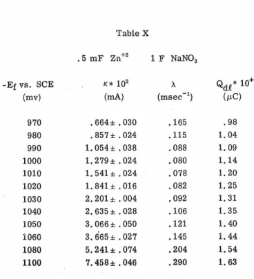
IV. Investigation of the Zn +2 /zn(Hg) Electrode Reaction in

Experimental Conditions

The solutions that were used for the measurements of the

kinetics of the reduction of zinc(II) ion at a mercury electrode were

always 1 F in supporting electrolyte, either NaN0₃, NaClO ₄ or NaCl,

and either 1 mF or . 5 mF in zinc ion. The electrode, a hanging

mercury drop, was renewed after every experimental run.

Each of the experiments was performed in the following manner:

The mercury electrode was initially potentiostated at -800 mV vs.

S. C. E. where no faradaic reaction occurred. The potential was then

stepped to a value where the faradaic reaction occurred and the

resulting charge-time response was recorded using the computer

system previously described. The potential to which the electrode

was stepped was varied over the range of -1000 mV to -1200 mV vs.

S. C. E. Data points were obtained every 500 µsec after the initiation

of the experiment until one hundred points had been obtained (50 msec).

To improve the precision of the data, ensemble averaging was

employed. Ensemble averaging was advantageous not only because it

improved precision but also because it cut down overall experimental

time. Although each set of data was obtained in 50 msec the analysis

of the data using non-linear least squares took several minutes.

Thus when several sets of data, generally four, were combined and

only the ensemble average analyzed quite a bit of time could be saved.

Ensemble averages of four runs were chosen because, when the