Passive modifications for partial assignment of natural frequencies of
mass-spring systems
Huajiang Ouyang1, Jiafan Zhang2
1
School of Engineering, University of Liverpool The Quadrangle, Liverpool L69 3GH, U.K.
2
School of Mechanical Engineering, Wuhan Polytechnic University Wuhan 430023, China
Abstract: The inverse structural modification for assigning a subset of natural frequencies of a structure to some targeted values has been found to inevitably lead to undesired changes to the other natural frequencies of the original structure that should not have been modified, which is referred to as the frequency “spill-over” phenomenon. Passive structural modifications of mass-spring systems for partial assignment of natural frequencies without frequency “spill-over” are addressed in this paper. For two kinds of lumped mass-spring systems, i.e. simply connected in-line mass-spring systems and multiple-connected mass-spring systems, two solution methods are proposed to construct the required mass-normalised stiffness matrix, which satisfies the partial assignment requirement of natural frequencies and maintains the configuration of the original structure after modifications. The modifications are also physically realisable. Finally, some examples of lumped mass-spring systems are analysed to demonstrate the effectiveness and accuracy of the proposed methods.
1. Introduction
2
SM is to predict modal properties as a result of structural modifications. The inverse SM problem, however, aims to determine the necessary structural modifications such that the modified structure has some prescribed desired dynamic behaviour, which usually involves an optimisation procedure looking for right modifications. As is well known, when the frequency of excitation is very close to a natural frequency excessive vibration occurs that may lead to structural failure. In this situation, it is useful to determine the changes of geometrical parameters (such as thickness, length, diameter, etc.) and/or material parameters (such as density, Young’s modulus, etc.), and/or consider the addition of any combination of lumped masses and stiffnesses in order to relocate the natural frequencies concerned to other locations. This inverse structural frequency modification problem is known as frequency (eigenvalue) placement or assignment.
Mathematically, it is closely related to inverse eigenvalue problems (IEP), which involve the specification of one or more eigenvalues of a matrix or a matrix pencil and the evaluation of how the elements of the matrix need to change to result in the prescribed eigenvalues. These problems have attracted much attention of researchers over the past thirty years.
1.1 Literature review
achieve the desired changes. It should be noted that even on frequency placement by structural modifications studied in this paper, there exist a large number of publications in the literature, and therefore only a brief review of some relevant papers is attempted below.
The methods for inverse structural modifications are based on the use of modal properties derived from a finite elements solution or experimental modal analysis. He [1], Sestieri and D’Ambrogio [2], and Nad [3] reviewed various structural modification methods. Tsuei and
Yee [4] described a method for shifting natural frequencies by using only measured frequency response data at modification points. This is particularly convenient and effective for modal testing. Mottershead [5], and his collaborators [6, 7] studied the relocation of an antiresonance and cancellation of a resonance with an antiresonance, and the assignment of natural frequencies and nodes of normal modes by the addition of grounded springs and concentrated masses using FRF data. Park and Park [8, 9] used FRF formulations to find analytically the necessary multiple mass, stiffness and damping modifications in order to exactly achieve both required eigenvalues and eigenvectors. For other related works based on FRF data, refer to [10–13].
4
and put forward an approximate method for calculating the modification matrices of the structure.
Fox and Kapoor [21] provided expressions of both eigenvalue and eigenvector sensitivities with respect to a design parameter, which can be expressed in terms of only the corresponding unmodified modal parameters and the structure's matrices. Smith and Hutton [22] discussed the use of Newton's method and inverse iteration of mode shape updating on the frequency modification in terms of first-order expansions of eigenvalues with respect to design variables. Farahani and Bahai [23] provided algorithms for relocating eigenvalues of structures based on eigenvalue sensitivities and their second-order expansions. Djoudi et al. [24] gave a formulation free from iterations for the inverse modification of bar and truss structures. Olsson and Lidström [25] considered constraints on structures when obtaining desired frequencies. The undamped natural frequencies of a constrained structure were calculated by solving a generalised eigenvalue problem derived from the equations of motion for the constrained system involving Lagrange multipliers. Smith and Hutton [26] and Kim et al. [27] solved inverse modification problems using perturbation theory.
frequencies of large-scale structures could be obtained accurately using the state-of-the-art techniques of matrix computations, or be measured using existing experimental facilities due to hardware limitations.
It should be mentioned that a necessary and sufficient condition was proposed for the incremental mass and stiffness matrices that modify some eigenpairs while keeping other eigenpairs unchanged in [28] but these matrices are not guaranteed to lead to physically realisable structural modifications. Additionally, there are several papers devoted to a related problem that a specific natural frequency of a structure does not change after mass and/or stiffness modifications. Çakar [29] studied a situation in which one of the pre-specified natural frequencies can be preserved by attaching a grounded spring to a structure after adding a number of masses to it. He developed a method based on the Sherman-Morrison formula in order to determine the necessary spring constant. Gürgöze and İnceoğlu [30] was concerned with satisfying a design objective such that the fundamental frequency of a cantilever beam remained the same in spite of the addition of a mass at some point on the beam. Mermertaş and Gürgöze [31] investigated the possibility of using springs to preserve the fundamental frequency of a thin rectangular plate carrying any number of point masses.
6
studied from both theoretical and computational view points, for example, see [32, 33]. To describe the dynamics of a structural system, usually a second-order differential equation is used, with structural matrices that are symmetric and sparse. However, transferring second-order equations to first-order configuration doubles the dimension of the system and the structural matrices lose some nice properties, such as positive semi-definiteness and sparsity, and even symmetry. Therefore, a large effort can be seen from the literature to have been made to tackle this problem directly on second-order dynamic system models over the past ten years, for example, see [34-39].
The capability of active control in making partial eigenvalue or eigenstructure assignment has been known. Obviously, it is desirable to make partial eigenvalue (or natural frequencies) assignment, without frequency “spill-over”, by means of passive control or passive structural modification (abbreviated as PEVAPSM in this paper) due to its advantage of low cost and maintenance of system stability. However, this is a far more difficult task. To the authors’ best knowledge, this has not been achieved before and is the major objective of this investigation.
1.2 Problem definition
Problem PEVAPSM: For an n-degree-of-freedom (DOF) undamped vibrating system
with a given theoretical model {𝐌0, 𝐊0}
,
a set of its associated eigenpairs (𝜆𝑖, 𝐱𝑖) (𝑖 =1,2, … , 𝑝) with 𝑝 < 𝑛
,
and another set of targeted (or modified) eigenvalues ( 𝜇𝑖) (𝑖 =1,2, … , 𝑝)
,
find a physically realisable n-DOF undamped vibrating system with thetheoretical model {𝐌, 𝐊}
, which has the same structured form as
{𝐌0, 𝐊0}, such that:
(1) The modified model {𝐌, 𝐊} now has eigenvalues ( 𝜇𝑖) (𝑖 = 1, 2, … , 𝑝);
(2) The remaining (unknown) 𝑛 − 𝑝 eigenvalues of the modified model {𝐌, 𝐊} are the same as those of the original model {𝐌0, 𝐊0}
.
where 𝐌0 , 𝐌, and 𝐊0, 𝐊 are, respectively, the mass and stiffness matrices of the models of the original and modified structures, and 𝐌0 = 𝐌0T > 𝟎, 𝐊0 = 𝐊0T ≥ 𝟎, 𝐌 = 𝐌T > 𝟎,
𝐊 = 𝐊T ≥ 𝟎
.
8
updating always leads to spill-over, while direct model updating usually does not result in physically realisable modifications.
Two kinds of lumped mass-spring systems are considered in this paper: (1) simply connected in-line mass-spring systems; (2) multiple-connected mass-spring systems. Their solutions are obtained from different numerical construction procedures. The former applies Lanczos method of tridiagonalisation reported in [42–44] to the real symmetric matrix constructed from the mass and stiffness matrices of the original structure and the eigenvalues to be assigned; while the latter exploits the gradient flow method for inverse eigenvalue problems with prescribed entries [45, 46]. In what follows, a real symmetric matrix satisfying the eigenvalue demands of PEVAPSM is constructed, and the solution of simply connected mass-spring systems is presented with a numerical example in Section 2. In Section 3, multiple-connected mass-spring vibrating systems are tackled, and the solution method and conditions for realising PEVAPSM are introduced with two numerical examples. Finally, some conclusions are drawn in Section 4.
2. PEVAPSM solution for simply connected mass-spring systems
2.1 Construction of a real symmetric matrix 𝐉𝑠
For an n-DOF undamped vibrating system with a given theoretical model {𝐌0,𝐊0}, its dynamics is characterised by the following eigenvalue equation:
(𝐊0− 𝜆𝐌0)𝐱 = 𝟎. (1)
Introducing 𝐃0 so that 𝐌0 = 𝐃02, and 𝐮 = 𝐃0𝐱, Eq.(1) is rewritten as follows:
𝐃0−1(𝐊0− 𝜆𝐃02)𝐃0−1𝐮 = 𝟎,
(𝐉0− 𝜆𝐈)𝐮 = 𝟎, (2)
where
𝐉0 = 𝐃0−1𝐊
0𝐃0−1.
(3)
𝐉0 is known as the mass-normalised stiffness matrix and it has the same eigenvalues as
{𝐌0,𝐊0}. For simply connected mass-spring systems (which means a mass is connected via a
spring to only an adjacent mass and the system is in the form of a chain of consecutive masses and springs; a mass is connected to at most two other masses), 𝐉0 is a Jacobi matrix in a tridiagonal form as follows:
[
1 1
1 2 2
1 1
0 0
0 0
0 0
n
n n
a b
b a b
b
b a
]
, (4)
where 𝑎𝑖 > 0, 𝑏𝑖 > 0.
In what follows, a real symmetric matrix 𝐉𝑠 is constructed first such that it has ( 𝜇𝑖) (𝑖 =
1, 2, … , 𝑝), and (𝜆𝑖 ) (𝑖 = 𝑝 + 1, 𝑝 + 2, … , 𝑛) (unmodified eigenvalues of {𝐌0,𝐊0}) as its
eigenvalues. Let
𝚲1 = diag(𝜆1, 𝜆2, ⋯ , 𝜆𝑝), 𝚲2 = diag(𝜆𝑝+1, 𝜆𝑝+2, ⋯ , 𝜆𝑛), 𝚺1 = diag(𝜇1, 𝜇2, ⋯ , 𝜇𝑝),
𝐗1= {𝐱1, 𝐱2, ⋯ , 𝐱𝑝}, 𝐗2 = {𝐱𝑝+1, 𝐱𝑝+2, ⋯ , 𝐱𝑛}. 𝐗 = ( 𝐗1 𝐗2) is the mass-normalised
eigenvector matrix of Eq.(1). Correspondingly, 𝐔 = (𝐔1 , 𝐔2 ) is the normalised eigenvector matrix of Eq.(2), partitioned corresponding to 𝐗1 and 𝐗2. From the spectral decomposition theorem of symmetric matrices [47], 𝐉𝑠 can be constructed as follows:
𝐉𝑠 = 𝐔1𝚺1𝐔1T+ 𝐔
2𝚲2𝐔2T. (5)
10
𝐉𝑠 = 𝐉0+ 𝐃0𝐗1 (𝚺1− 𝚲1)𝐗1T𝐃
0. (6)
Note that (1) the constructed matrix 𝐉𝑠 has the same eigenvectors as 𝐉0; (2) 𝐉𝑠 usually is not in a Jacobi matrix form as in (4), and thus a physically realisable simply connected mass-spring system cannot be reconstructed from 𝐉𝑠. This calls for an alternative mass-normalised reconstructed stiffness matrix 𝐉 = 𝐃−𝟏𝐊𝐃−𝟏 that possesses the same eigenvalues as 𝐉𝒔 and at the same time is in a Jacobi form (4) (so that the modifications will be physically realisable), where 𝐃𝟐 = 𝐌,and 𝐌 and 𝐊 are mass and stiffness matrices of the modified system, respectively.
2.2 Tridiagonalisation of 𝐉𝒔 using Lanczos algorithm
The Lanczos algorithm has often been used to reduce symmetric matrices to tridiagonal form in order to solve for their eigenvalues. A variation of it is also used to solve inverse eigenvalue problems of vibrating systems [42, 47], which is employed here. This variation is based on the idea of producing the orthogonal similarity transformationformula as follows:
𝐉 = 𝐕T𝐉
𝑠𝐕 or 𝐕𝐉 = 𝐉𝑠𝐕, (7)
Here 𝐕 is an orthogonal matrix and it is built up column by column from 𝐉𝑠. It is known that, if 𝐉𝑠 is positive semi-definite, its eigenvalues are all distinct, and the initial vector 𝐯1 (i.e. the first column of V) is not orthogonal to any eigenvector of 𝐉𝑠, then the algorithm will result in a unique Jacobi matrix (4) for a given 𝐯1 [42]. Additionally, this algorithm has the advantage that numerically it is well conditioned. Now, the algorithm is outlined as follows:
Output: a Jacobi matrix 𝐉 in the form of (4) and an orthogonal matrix
𝐕 = (𝐯1, 𝐯2 , … , 𝐯𝑛) such that 𝐉 = 𝐕T𝐉𝑠𝐕.
(1) set 𝑎1∶= 𝐯1T𝐉𝑠𝐯1 (2) for 𝑖 = 1, 2, … , 𝑛 − 1
if 𝑖 = 1 then 𝐳1 = 𝑎1𝐯1− 𝐉𝑠𝐯1, 𝑏1 = √𝐳1T𝐳1 , 𝐯2 = 𝐳1⁄𝑏1.
else 𝑎𝑖 = 𝐯𝑖T𝐉𝑠𝐯𝑖, 𝐳𝑖 = 𝑎𝑖𝐯𝑖− 𝑏𝑖−1𝐯𝑖−1− 𝐉𝑠𝐯𝑖, 𝑏𝑖 = √𝐳𝑖T𝐳𝑖 , 𝐯𝑖+1= 𝐳𝑖⁄𝑏𝑖. end if
end for
(3) set 𝑎𝑛∶= 𝐯𝑛T𝐉𝑠𝐯𝑛.
Note that, for a given matrix 𝐉𝑠, the resultant Jacobi matrix 𝐉 from the above algorithm is not unique due to randomly chosen initial Lanczos vector 𝐯1.
2.3 Reconstruction of mass-spring systems solving PEVAPSM
12
𝐌 =
1 2
0 0 0
0 0 0
0 0 0 n
m m m
,𝐊 =
1 2 2
2 2 3 3
1 1 0 0 0 0 0 0 0 0 0 0
n n n n
n n
k k k
k k k k
k k k k
k k (8)
Let 𝐪1 = (1, 1, … ,1 )T, one has
𝐊𝐪1 = (𝑘1, 0, … ,0 )T. (9)
Since 𝐊 = 𝐃𝐉𝐃, one has
𝐃𝐉𝐃𝐪1 = 𝐃𝐉𝐃(1, 1, … ,1 )T = (𝑘1, 0, … ,0 )T, (10)
where 𝐃 = 𝐌1 2⁄ = diag(√𝑚1, √𝑚2 , … , √𝑚𝑛). Then Eq.(10) is rewritten as
𝐉(√𝑚1, √𝑚2 , … , √𝑚𝑛) T
= (𝑘1⁄√𝑚1, 0, … ,0 )T. (11)
Since the previously given Jacobi matrix 𝐉 is non-singular, it is known that its inverse matrix 𝐉−1 is a strictly positive matrix, meaning that each element of 𝐉−1 is strictly positive
[43]. Therefore, it is guaranteed that (√𝑚1, √𝑚2 , … , √𝑚𝑛) T
solved from Eq.(11) will be a strictly positive vector.
Now, take the obtained non-singular 𝐉 in Section 2.2 and solve 𝐉𝐪 = (1, 0, … ,0 )T for 𝐪. The solution 𝐪 is strictly positive. Thus the solution of Eq.(11) can be rewritten as
(√𝑚1, √𝑚2 , … , √𝑚𝑛) T
= 𝑐𝐪, (12)
where 𝑐 > 0 is to be determined from other considerations, for example, one can assume the total mass of a structure remains unchanged or should not exceed a certain value.
Suppose that the total mass of the system is m. Then
𝑚 = ∑𝑛 𝑚𝑖 =
𝑖=1 𝑐2𝐪𝐪T. (13)
diag(√𝑚1, √𝑚2 , … , √𝑚𝑛) from (12). Then 𝐊 = 𝐃𝐉𝐃 completes the reconstruction for
the “fixed-free” system. For details of the reconstruction for other types of systems, refer to [43, 44].
The above discussion shows the existence of a meaningful solution of PEVAPSM for simply connected mass-spring systems and how to find it. A numerical example is presented below.
Example 2.1: a five-DOF “fixed-free” type of simply connected mass-spring system, as shown in Fig.1, with {𝐌0,𝐊0} as follows:
0
1 0 0 0 0
0 1 0 0 0
0 0 1 0 0
0 0 0 1 0
0 0 0 0 1
M , 0
2 1 0 0 0
1 2 1 0 0
0 1 2 1 0
0 0 1 2 1
0 0 0 1 1
K .
Its eigenvalues (or natural frequencies squared) are λ = {0.0810, 0.6903, 1.7154, 2.8308, 3.6825}, respectively. The first two eigenvalues 𝚲1 = diag(0.0810, 0.6903) are required to become 𝚺1 = diag(0.15, 0.95), and the other eigenvalues remain unchanged. It is assumed that the total mass of the system remains unchanged too after the modification. The mass-normalised modal matrix 𝐗1 corresponding to 𝚲1 is
1
0.1699 0.4557
0.3260 0.5969
0.4557 0.3260
0.5485 0.1699
0.5969 0.5485
X .
The obtained matrices 𝐉𝑠 and 𝐉 are, respectively,
𝐉s=
(
2.0559 − 0.9255 0.0439 − 0.0137 − 0.0579 −0.9255 2.0999 − 0.9392 − 0.0140 − 0.0716 0.0439 − 0.9392 2.0419 − 0.9971 − 0.0277 −0.0137 − 0.0140 − 0.9971 2.0283 − 0.9532 −0.0579 − 0.0716 − 0.0277 − 0.9532 1.1027)
14
𝐉 =
(
2.5231 1.0909
1.0909 2.4089 0.7028
0.7028 1.2693 0.7848
0.7848 1.7352 1.0278
0 0 0
0 0
0 0
0 0
0 0 0 1.0278 1.3922
)
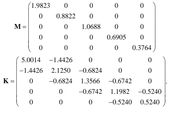
The modified mass and stiffness matrices constructed from 𝐉 are, respectively,
0 0 0 0
0 0 0 0
0 0 0 0
0 0 0 0
0 1.9823 0.8822 1.0688 0.6905 0.37
0 0 0 64
M 5.0014 1.4426
1.4426 2.1250 0.6824
0.6824 1.3566 0.6742
0.6742 1.1982 0.5240 0.5240 0
0 0 0
0 0
0 0
.52
0 0
0 0 0 40
K .
[image:14.595.152.446.197.395.2]The new masses and spring constants that make the partial frequency assignment are given in the brackets in Fig. 1.
Figure 1. A five-DOF “fixed-free” type of original mass-spring system and modified system
3. PEVAPSM solution for multiple-connected mass-spring systems
3.1 Matrix structures of mass and stiffness matrices
For multiple-connected mass-spring systems, the matrix structure of mass matrix 𝐌 remains unchanged: it is real, positive and diagonal. However, the matrix structure of stiffness matrix 𝐊 varies according to different configurations of the connectivity of masses and springs, except that 𝐊 is real symmetric and positive semi-definite. Additionally, stiffness matrix 𝐊 = (𝑘𝑖𝑗) has the following properties:
weakly diagonally dominant;
(2) If there is a spring, denoted by 𝑖ℓ, between the a-th mass and the b-th mass, then the entries 𝑘𝑎𝑏 and 𝑘𝑏𝑎 of 𝐊 are given by – 𝑘𝑖ℓ, where 𝑘𝑖ℓ is the stiffness of spring 𝑖ℓ. Otherwise 𝑘𝑎𝑏 = 𝑘𝑏𝑎 = 0. If the a-th mass is connected to springs 𝑗1, … , 𝑗ℎ, then 𝑘𝑎𝑎 =
∑ℎ 𝑘𝑗𝑠
𝑠=1 .
The mass-normalised stiffness matrix 𝐉 = 𝐃−1𝐊𝐃−1 of a multiple-connected mass-spring system has the same matrix structure as stiffness matrix 𝐊, it is real symmetric and positive semi-definite with the same zero entry patterns as 𝐊. Here 𝐉 is no longer in a Jacobi matrix form as (4) either, and may take the widely populated form, for example, for a general lumped mass-spring system as follows:
𝐉 =
11 1 12 1 2 13 1 3 1 1
12 1 2 22 2 23 2 3 2 2
13 1 3 23 2 3 33 3 3 3
1 1 2 2 3 3
n n
n n
n n
n n n n n n nn n
k m k m m k m m k m m
k m m k m k m m k m m
k m m k m m k m k m m
k m m k m m k m m k m
. (14)
3.2 Inverse eigenvalue problem and the gradient flow method 3.2.1 Problem description
16
multiple connected mass-spring system {𝐌0,𝐊0}). It implies that one cannot physically reconstruct a multiple-connected mass-spring system while keeping the configuration of the structure unchanged in solving PEVAPSM. To overcome this problem, one naturally tries to convert the obtained 𝐉𝑠 into a matrix 𝐉 through orthogonal similarity transforms such that 𝐉 has the same matrix structure as 𝐉0. Thus the resultant 𝐉 can become the mass-normalised stiffness matrix of a new system {𝐌, 𝐊}, and one can reconstruct this new multiple-connected mass–spring system from 𝐉 with the same configuration of the structure as that of the original system.
Toward this end, a special type of IEP, matrix completion with prescribed eigenvalues [45, 46], is briefly discussed here, and a numerical algorithm, the gradient flow method, which was used to tackle such an IEP, is exploited to achieve the goal mentioned above.
The goal of matrix completion is to construct a matrix subject to both the structural constraint of prescribed entries and the spectral constraint of prescribed eigenvalues. This special kind of IEP corresponds to the circumstance that “a portion of the physical system is known a priori, a portion of the matrix to be constructed has fixed entries. The prescribed entries are used to characterise the underlying structure. The task is to specify values for the remaining entries so that the completed matrix has prescribed eigenvalues”, as indicated in
the same as those of 𝐉0. Thus, the problem is now converted into the completion of matrix 𝐉 with prescribed eigenvalues of matrix 𝐉𝑠.
Unfortunately, very few theories or numerical algorithms are available for solving such an IEP. The challenge lies in the intertwining of the cardinality and the locations of the prescribed matrix entries so that the inverse problem is solvable. Chu et al. [45] recast the matrix completion problem as minimising the distance between the isospectral matrices (i.e. those matrices with the same eigenvalues) with the prescribed eigenvalues and the affined matrices with the prescribed entries, and then finding the intersection of them. As the gradient of the objective function can be explicitly calculated, a steepest descent gradient flow therefore can be formulated. By integrating this gradient flow numerically, they developed a way to tackle the matrix completion problem. Additionally, this gradient flow method is general enough that it can be used to explore the question on existence of a solution when the prescribed matrix entries are set at some particular locations with some corresponding cardinalities, such as the case of constructing structured matrix 𝐉 discussed in this subsection. In what follows the gradient flow method of matrix completion is outlined.
3.2.2 The gradient flow method
The gradient flow method proposed in [45] is for a general real matrix completion, which is presented in the simplified form for a real symmetric matrix completion as follows.
Let 𝐖 ∈𝑛×𝑛 denotes a real symmetric matrix with distinct eigenvalues {1,2 , … ,𝑛}.
The set
18
consists of all matrices that are isospectral to 𝐖. Given an index subset of locations
𝒦 = {(𝑖ν , 𝑗ν)}ν=1ℓ and the prescribed values 𝐠 = {𝑔
1, 𝑔2 , … , 𝑔ℓ}, the set
ℵ(𝒦, 𝐠 ) = {𝐀 ∈𝑛×𝑛 | A
𝑖ν𝑗ν = 𝑔ν , ν = 1, … , ℓ} (16)
contains all matrices with the prescribed entries at the desired locations. For convenience, split any given matrix 𝐘 in 𝔐(𝐖) as the sum
𝐘 = 𝐘𝒦 + 𝐘𝒦𝑐, (17)
where entries in 𝐘𝒦 are the same as 𝐘, except those entries that do not belong to 𝒦 are set identically zero; and 𝒦𝑐 is simply the index subset complementary to 𝒦. With respect to the Frobenius inner product
〈𝐁, 𝐃〉 = ∑𝑛𝑖,𝑗=1𝑏𝑖𝑗𝑑𝑖𝑗 , (18)
the projection 𝑃(𝐘) of any matrix 𝐘 onto the affine subspace ℵ(𝒦, 𝐠 ) is given by
𝑃(𝐘) = 𝐀𝒦 + 𝐘𝒦𝑐, (19)
where 𝐀𝒦 is a constant matrix in ℵ(𝒦, 𝐠 ) with zero entries at all locations corresponding to 𝒦𝑐. For each given 𝐘 ∈ 𝔐(𝐖), it is intended to minimise the distance between 𝐘 and
ℵ(𝒦, 𝐠 ). Equivalently, it is to minimise the function defined by
𝑓(𝐘) =12〈𝐘 − 𝑃(𝐘), 𝐘 − 𝑃(𝐘)〉, (20)
where 𝐘 − 𝑃(𝐘) = 𝐘𝒦− 𝐀𝒦.
Let 𝐘 = 𝐕𝐖𝐕T. This minimisation with objective function 𝑓(𝐘) can be rewritten as an unconstrained optimisation problem in terms of 𝐕 as follows:
ℎ(𝐕) =12〈𝐕𝐖𝐕T− 𝑃(𝐕𝐖𝐕T), 𝐕𝐖𝐕T− 𝑃(𝐕𝐖𝐕T)〉. (21)
The gradient ∇ℎ of objective function ℎ is given by [45]
Post-multiplying Eq.(22) by 𝐕T , one obtains
∇ℎ(𝐕)𝐕T = [𝐘 − 𝑃(𝐘), 𝐘T], (23)
where [𝐘 − 𝑃(𝐘), 𝐘T] denotes the Lie bracket commutator, i.e. [𝐁, 𝐃] = 𝐁𝐃 − 𝐃𝐁, and
𝐘 = 𝐕𝐖𝐕T. It follows that the vector field 𝑑𝐕
𝑑𝑡 = [ 𝐘
T, 𝐘 − 𝑃(𝐘)]𝐕 (24)
defines a gradient flow of ℎ(𝐕) in the open set consisting of n × n orthogonal matrices and moves in the steepest descent direction to reduce the value of ℎ(𝐕) [45]. The system of ordinary differential equations (24) can be readily integrated from a starting point, say,
𝐕(0) = 𝐈 (the identity matrix). ∇ℎ(𝐕(𝑡)) will converge to zero as t goes to infinity,
implying that a local minimum for ℎ(𝐕) has been found. The integration stop criterion of Eq.(24) can be chosen as follows:
min {‖𝐘(𝑡𝑘) − 𝑃(𝐘(𝑡𝑘))‖𝐹 , ‖[𝐘(𝑡𝑘)T, 𝐘(𝑡𝑘) − 𝑃(𝐘(𝑡𝑘))]‖𝐹} ≤ 10−8, (25)
where ‖∙‖F denotes the Frobenius norm of a matrix. It should be noted that, in the event that a solution does not exist, the formulation enables one to find a least-squares solution.
3.3 Numerical examples of PEVAPSM solution
Based on the above discussion, PEVAPSM solutions of two multiple-connected mass-spring systems are presented for the purpose of demonstration in the following. One is a simple 4-DOF system and the other a more complex 10-DOF one. The existing ordinary differential equation solver ode15s in Matlab is used to implement the computation in this subsection. To control the integration, local tolerance values of AbsTol = 10−10 and
20 Matlab codes.
Example 3.1. a 4-DOF mass-spring system, as shown in Fig.2, with {𝐌0,𝐊0} as follows:
𝐌0 = 1
2 3
4
0 0 0
0 0 0
0 0 0
0 0 0
m m m m
, 𝐊0 =
1 2 5 2 5
2 2 3 3
5 3 3 4 5 4
4 4
0
0
0 0
k k k k k
k k k k
k k k k k k
k k .
Let 𝑚1 = 𝑚2 = 𝑚3 = 𝑚4 = 1.0 and 𝑘1 = 𝑘2 = 𝑘3 = 𝑘4 = 𝑘5 = 1.0. Its eigenvalues (or natural frequencies squared) are λ = {0.1783,1.1538,3.4882,4.1796}, respectively. The first
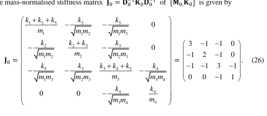
two eigenvalues 𝚲1 = diag(0.1783,1.1538) are required to relocate to 𝚺1 = diag(0.5, 1.5), and the other eigenvalues remain unchanged. 𝐗1 is not listed for the sake of saving space. The mass-normalised stiffness matrix 𝐉0 = 𝐃0−1𝐊0𝐃0−1 of {𝐌0,𝐊0} is given by
𝐉0 =
1 2 5 2 5
1 1 2 1 3
2 2 3 3
2
1 2 2 3
5 3 3 4 5 4
3
1 3 2 3 3 4
4 4 4 3 4 0 0 0 0
k k k k k
m m m m m
k k k k
m
m m m m
k k k k k k
m
m m m m m m
k k m m m =
3 1 1 0
1 2 1 0
1 1 3 1
0 0 1 1
[image:20.595.86.517.350.537.2]. (26)
Figure 2. A 4-DOF “fixed-free” type of multiple connected mass-spring system
The constructed real symmetric matrix 𝐉𝑠 from the formula (6) in Section 2.1 is given by
𝐉𝑠 =
3.0862 0.8745 0.9280 0.0225
0.8745 2.1835 0.8998 0.0478
0.9280 0.8998 3.0890 0.9252
0.0225 0.0478 0.9252 1.3091
. (27)
structure is not the same as that of 𝐉0, which means one cannot reconstruct the modified system directly from 𝐉𝑠 with the same configuration structure as {𝐌0,𝐊0}.
Now, the mass-normalised stiffness matrix 𝐉 of the modified system with the same matrix structure as 𝐉0 and the same eigenvalues as 𝐉𝑠 is to be constructed using the gradient flow method of the matrix completion discussed in subsection 3.2.2. Let some non-zero entries of
𝐉 be set to be known a priori. For example, suppose modified values of 𝑚3, 𝑚4 and 𝑘4 are
prescribed a priori, or for convenience, their values are left unchanged, i.e. 𝑚̃3 = 𝑚̃4 =
1.0, 𝑘̃4 = 1.0, which means 𝐉(3,4) = 𝐉(4,3) = −1, 𝐉(4,4) = 1. Additionally, let zero entry
pattern of 𝐉 be the same as that of 𝐉0, which means 𝐉(1,4) = 𝐉(2,4) = 𝐉(4,1) = 𝐉(4,2) = 0. At this point, using notation in subsection 3.2.2, one has
𝐀𝒦 =
0
0
1
0 0 1 1
, 𝐖 = 𝐉𝑠,
where the stars in 𝐀𝒦 indicate unknown entries to be determined. Set 𝐕(0) = 𝐈 (a 4 × 4 identity matrix), and start with 𝐘0 = 𝐕(0)𝐉𝑠𝐕(0)T = 𝐉𝑠.
The gradient flow method gives 𝐉 = 𝐘 = 𝐕𝐉𝑠𝐕T as follows:
𝐉 =
3.0933 0.8264 0.7768
0.8264 2.2711 0.6801
0.7768 0.6801 3.3034 0
0
1
0 0 1 1
. (28)
It is easily verified that the obtained 𝐉 has eigenvalues {0.5,1.5,3.4882,4.1796}.
22
Take 𝐪 = (1, 1, … ,1 )T as the static displacements of all the masses, one has
𝐊𝐪 = (𝑘̃1, 0, … ,0 )T (29)
𝐮 = 𝐃𝐪 = 𝐌1 2⁄ 𝐪 = (𝑚̃ 1 1 2⁄ , 𝑚̃
2 1 2⁄ , 𝑚̃
31 2⁄ , 𝑚̃41 2⁄ ) T
(30)
𝐉𝐮 = 𝐌−1 2⁄ 𝐊𝐌−1 2⁄ 𝐌1 2⁄ 𝐪 = 𝐌−1 2⁄ 𝐊𝐪 = (𝑘̃
1/√𝑚̃1, 0,0,0) T
(31)
Substituting 𝐉 of (28) into (31), expanding the first three equations of (31), one has
1 2 1 2 1 2
1 2 3 1 1
1 2 1 2 1 2
1 2 3
1 2 1 2 1 2 1 2
1 2 3 4
3.0933 0.8264 0.7768
0.8264 2.2711 0.6801 0
0.7768 0.6801 3.3034 0
m m m k m
m m m
m m m m
. (32)
Simultaneously solving the second and third equation of (32) in terms of 𝑚̃3 = 𝑚̃4 = 1.0,
one gets 𝑚̃1 and 𝑚̃2. Substituting them into the first equation of (32), one gets 𝑘̃1. Because entries 𝐉(1,2) = k2 m m1 2 = 0.8264 , 𝐉(1,3) = k5 m m1 3 = 0.7768 , 𝐉(2,2) =
2 3 2
(k k ) m = 2.2711, one obtains 𝑘̃2, 𝑘̃3, and 𝑘̃5. Thus one has entire physical parameters of the modified system, as shown in Table 1.
Table 1. Masses and spring constants of the original and modified structures (𝑚̃1−4 and 𝑘̃1−5)
𝑚1 𝑚2 𝑚3 𝑚4 𝑘1 𝑘2 𝑘3 𝑘4 𝑘5
1.0 1.0 1.0 1.0 1.0 1.0 1.0 1.0 1.0 𝑚̃1 𝑚̃2 𝑚̃3 𝑚̃4 𝑘̃1 𝑘̃2 𝑘̃3 𝑘̃4 𝑘̃5 4.2024 1.0929 1.0 1.0 9.6359 1.7710 0.7110 1.0 1.5924
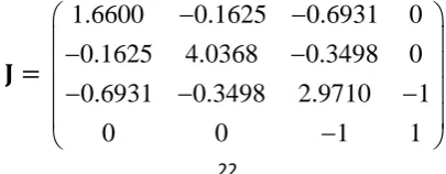
It is worthwhile to note that (1) if 𝐕(0) is chosen to be an arbitrary orthogonal matrix, the gradient flow method would ends at a different limit point, such as
𝐉 =
1.6600 0.1625 0.6931
0.1625 4.0368 0.3498
0.6931 0.3498 2.9710
0
0
1
0 0 1 1
[image:22.595.194.397.699.778.2]which means one can reconstruct another PEVAPSM solution of the original system from
𝐉 above; (2) if other non-zero entries of 𝐉 are set to be known a priori, one can also
reconstruct different PEVAPSM solutions.
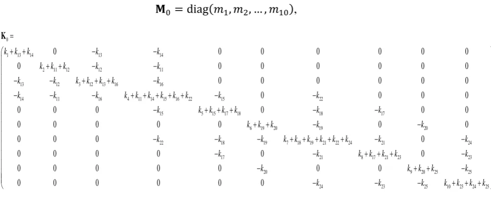
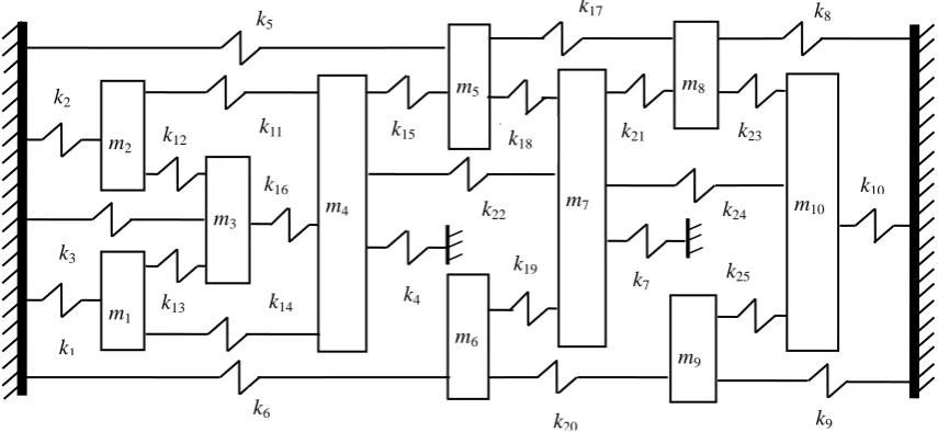
Example 3.2. a 10-DOF mass-spring system [48], as shown in Fig.3, with {𝐌0,𝐊0} as follows:
𝐌0 = diag(𝑚1, 𝑚2, … , 𝑚10),
0
1 13 14 13 14
2 11 12 12 11
13 12 3 12 13 16 16
14 11 16 4 11 14 15 16 22 15 22
15 5 15 17 18 18 17
6 19 20 19 20
22 18
0 0 0 0 0 0 0
0 0 0 0 0 0 0
0 0 0 0 0 0
0 0 0 0
0 0 0 0 0 0
0 0 0 0 0 0 0
0 0 0
k k k k k
k k k k k k k k k k k k
k k k k k k k k k k k
k k k k k k k
k k k k k
k k K
19 7 18 19 21 22 24 21 24
17 21 8 17 21 23 23
20 9 20 25 25
24 23 25 10 23 24 25
0
0 0 0 0 0 0
0 0 0 0 0 0 0
0 0 0 0 0 0
k k k k k k k k k
k k k k k k k
k k k k k
k k k k k k k
All spring constants are 2.4 × 10⁵N m⁄ , and 𝑚1 = 30kg, 𝑚2 = 35kg, 𝑚3 = 40kg, 𝑚4 =
45kg, 𝑚5 = 45kg, 𝑚6 = 45kg, 𝑚7 = 40kg, 𝑚8 = 35kg, 𝑚9 = 30kg, 𝑚10= 25kg . Its
eigenvalues (or natural frequencies squared) are λ = {6298.12,9628.31,14109.22,22117.92,
22733.69, 27718.30, 32139.94, 35557.23, 42219.32, 49077.96}, respectively. The first two
eigenvalues 𝚲1 = diag(6298.12,9628.31) are required to relocate to
𝚺1 = diag(9012,12118), and the other eigenvalues remain unchanged. 𝐗1, 𝐉0 and 𝐉𝑠
[image:23.595.72.562.235.435.2]are not listed for the sake of saving space.
24
The matrix structure of the obtained 𝐉𝑠 is not the same as that of 𝐉0 either, which means one cannot reconstruct the modified system directly from 𝐉𝑠 with the same configuration structure as {𝐌0,𝐊0}. Now, the mass-normalised stiffness matrix 𝐉 of the modified system with the same matrix structure as 𝐉0 and the same eigenvalues as 𝐉𝑠 is to be constructed using the gradient flow method of matrix completion. Sometimes it is convenient to allow some entries of 𝐉, for example, 𝐉(9, 9) = (𝑘̃9+ 𝑘̃20+ 𝑘̃25) 𝑚⁄̃9, 𝐉(9, 10) = 𝐉(10, 9) =
−𝑘̃25⁄√𝑚̃9𝑚̃10 , 𝐉(8, 10) = 𝐉(10, 8) = −𝑘̃23⁄√𝑚̃8𝑚̃10 , 𝐉(7, 10) = 𝐉(10, 7) =
−𝑘̃24⁄√𝑚̃7𝑚̃10 , and 𝐉(10, 10) = (𝑘̃10+ 𝑘̃23+ 𝑘̃24+ 𝑘̃25) 𝑚⁄̃10, to be equal to the
corresponding entries of 𝐉0. The mathematical expressions of these entries of 𝐉 are explicitly given to aid understanding of their physical meanings . Meanwhile, let zero entry pattern of 𝐉 be the same as that of 𝐉0. Thus one has
𝐀𝒦 =
0 0
0 0
0 0 0 0
0 0 0 0 0 0 0
0 0 0 0 0 0 0
0 0 0 0 0 0
0 0 0 0
0 0 0 0 0 0
0 0 0 0 0 0 0
0 0 0 0 7,10
0 0 0 0 0 0 8,10
0 0 0 0 0 0 0 9, 9 9,10
0 0 0 0 0 0 10, 7 10,8 10, 9 10,10
J J
J J
J J J J
.
Set 𝐕(0) = 𝐈 (a 10 × 10 identity matrix), and start with 𝐘0 = 𝐕(0)𝐉𝑠𝐕(0)T = 𝐉𝑠, the gradient flow method gives 𝐉 = 𝐘 = 𝐕𝐉𝑠𝐕T as follows:
2.4090e+4 0 -6.4017e+3 -5.8373e+3 0 0 0 0 0 0
0 2.0638e+4 -5.5792e+3 -4.7904e+3 0 0 0 0 0 0
-6.4017e+3 -5.5792e+3 2.5478e+4 -4.1434e+3 0 0 0 0 0 0
-5.8373e+3 -4.7904e+3 -4.1434e+3 3.3804e+4 -4.6084e+3 0 -4.3752e+3 0 0 0
0 0 0 -4.6084e+3 1.8417e+4 0 -2.0021e+3 -7.3117e+3 0 0
0 0 0 0 0 1.7552e+4 -3.0753e+3 0 -5.9524e+3 0
0 0 0 -4.3752e+3 -2.0021e+3 -3.0753e+3 3.8423e+4 -5.6127e+3 0 -7.5895e+3
0 0 0 0 -7.3117e+3 0 -5.6127e+3 2.6001e+4 0 -8.1135e+3
0 0 0 0 0 -5.9524e+3 0 0 2.4000e+4 -8.7636e+3
0 0 0 0 0 0 -7.5895e+3 -8.1135e+3 -8.7636e+3 3.8400e+4
It should be noted that the entries with numerical values in the orders of 10−11 or below in
the above matrix 𝐉 are already set to be zero.
Now, one can reconstruct the modified mass-spring system with the same configuration structure as {𝐌0,𝐊0}, shown in Fig.3, from 𝐉. Similar to (29)-(31), one has
𝐉(𝑚̃11 2⁄ , 𝑚̃21 2⁄ , … , 𝑚̃101 2⁄ )T = (𝑘̃1/√𝑚̃1, 𝑘̃2/√𝑚̃2, … , 𝑘̃10/√𝑚̃10)T. (33)
At this point, a different reconstruction procedure for physical parameters is used. One can prescribe values of the entries of the right-hand vector in Eq.(33). Here the ratios of
𝑘̃1/√𝑚̃1, 𝑘̃2/√𝑚̃2, … , 𝑘̃10/√𝑚̃10 are taken to be the same as that of the original system.
Then solving Eq.(33), one has 𝐃 = 𝐌1 2⁄ = diag(𝑚̃11 2⁄ , 𝑚̃21 2⁄ , … , 𝑚̃101 2⁄ ), and subsequently
𝐊 = 𝐃𝐉𝐃. The results are listed as follows:
𝐌 = diag(14.620, 15.591, 15.641, 15.492, 27.244, 17.019, 12.720, 25.479, 18.588, 16.043),
𝐊 =
e+5 0 - e+4 -8.7850e+4 0 0 0 0 0 0
0 3.2175e+5 -8.7124e+4 -7.4449e+4 0 0 0 0 0 0
-9.6806e+4 -8.7124e+4 3.9851e+5 -6.4498e+4 0 0 0 0 0 0
-8.7850e+4 -7.4449e+4 -6.4498e+4 5.2371e+5 -9.4676e+4 0 -6.1418e+4 0 0 0
0 0 0 -9.
3.5220 9.680
4676e+ 6
4 5.0174e+5 0 -3.7269e+4 1.9264e+5 0 0
0 0 0 0 0 2.9871e+5 -4.5246e+4 0 -1.0587e+5 0
0 0 0 -6.1418e+4 -3.7269e+4 -4.5246e+4 4.8873e+5 -1.0104e+5 0 -1.0841e+5
0 0 0 0 -1.9264e+5 0 -1.0104e+5 6.6248e+5 0 -1.6403e+5
0 0 0 0 0 -1.0587e+5 0 0 4.4612e+5 -1
-.5134e+5
0 0 0 0 0 0 -1.0841e+5 -1.6403e+5 -1.5134e+5 6.1604e+5
This modified system {𝐌, 𝐊} accurately assigns the first two eigenvalues to
26
errors of the remaining eigenvalues between {𝐌, 𝐊} and {𝐌0,𝐊0} are listed in Table 2. Table 2. The absolute errors of the remaining eigenvalues
|𝜇3− 𝜆3| |𝜇4− 𝜆4| |𝜇5− 𝜆5| |𝜇6− 𝜆6| |𝜇7− 𝜆7| |𝜇8− 𝜆8| |𝜇9− 𝜆9| |𝜇10− 𝜆10|
1.1879e-5 1.5775e-6 6.7383e-5 6.2182e-6 2.2771e-6 3.8391e-5 1.0212e-5 1.0869e-5
which indicates an excellent assignment.
Clearly, the PEVAPSM solution of this 10-DOF multiple-connected mass-spring system is not unique either. Additionally, it should be pointed out firstly that according to Eq. (5) (i.e. a real symmetric matrix Js constructed), the spectral orders of the eigenvalues of the original
system to be assigned before assignment must be in the same spectral orders of the modified
system after assignment. Secondly, the first method based on Lanczos algorithm is just
applicable to the simply connected systems and is computationally effective; while the
second method based on the gradient flow algorithm is applicable to both systems, but is
computationally more expensive for large systems.
4. Conclusions
stiffness matrix, which satisfies the partial assignment requirement of natural frequencies and at the same time keeps the structural configuration of the original system, that is, the structure of the mass and stiffness matrices remains unchanged after modifications. The methods only need information of those few eigenpairs to be assigned and the analytical mass and stiffness matrices of the original system. Their solutions are not unique and dependent on the prescribed conditions on the physical parameters of masses and springs of the modified system.
For continuous structures (or distributed systems), quite often lumped mass matrices are used in the finite element discretisation, and the methods put forward in this paper are also applicable.
The methods also allow other design constraints to be considered, for example, maintenance of the total mass. Structural optimisation with partial eigenvalue assignment can be carried out.
It will be a challenge to be able to deal with non-diagonal mass matrices (for example, consistent mass matrices in the FEM). This will be the authors’ next research topic.
Acknowledgements
28
References
[1] He, J. 2001 Structural modification. Philosophical Transactions of the Royal Society of London A 359,187-204.
[2] Sestieri, A. & D’Ambrogio, W. 2001 Structural dynamic modification. Encyclopedia of Vibration. London: Academic Press; 1253-1264.
[3] Nad, M. 2007 Structural dynamic modification of vibrating systems. Applied and Computational Mechanics 1, 203-214.
[4] Tsuei, Y. G. & Yee, E. K. L. 1989 A method to modify dynamic properties of undamped mechanical systems. ASME Journal of Dynamic Systems, Measurement and Control 111, 403–408.
[5] Mottershead, J.E. 2001 Structural modification for the assignment of zeros using measured receptances. ASME Journal of Applied Mechanics 68, 791–798.
[6] Mottershead, J. E., Mares, C. & Friswell, M. I. 2001 An inverse method for the assignment of vibration nodes. Mechanical Systems and Signal Processing 15 (1): 87–100.
[7] Mottershead, J. E. & Lallement, G. 1998 Vibration nodes, and the cancellation of poles and zeros by unit-rank modifications to structures. Journal of Sound and Vibration 222 (5): 833–851.
[8] Park, Y. H. & Park, Y. S. 2000 Structural modification based on measured frequency response functions: An exact eigen properties reallocation. Journal of Sound and Vibration 237 (3): 411–426.
[9] Park, Y. H. & Park, Y. S. 2000 Structure optimization to enhance its natural frequencies based on measured frequency response functions. Journal of Sound and Vibration 229 (5): 1235–1255.
[10] Kyprianou, A., Mottershead, J. E. & Ouyang, H. 2005 Structural modification. Part 2: assignment of natural frequencies and antiresonances by an added beam. Journal of Sound and Vibration 284 (1–2), 267–281.
frequencies by an added mass and one or more springs. Mechanical Systems and Signal Processing 18 (2), 263–289.
[12] Ouyang, H. 2009 Prediction and assignment of latent roots of damped asymmetric systems by structural modifications. Mechanical Systems and Signal Processing 23 (6), 1920 –1930.
[13] Ouyang, H., Richiedei, D., Trevisani, A. & Zanardo, G. 2012 Eigenstructure assignment in undamped vibrating systems: a convex-constrained modification method based on receptances. Mechanical Systems and Signal Processing 27 (2): 397–409.
[14] Bucher, I. & Braun, S. G. 1993 The structural modification inverse problem: an exact solution. Mechanical Systems and Signal Processing 7 (1), 217-238.
[15] Sivan, D. & Ram, Y. M. 1996 Mass and stiffness modification to achieve desired natural frequencies. Communication in Numerical Methods in Engineering 12, 531–42. [16] Ram, Y. M. 1994 Enlarging a spectral gap by structural modification. Journal of Sound
and Vibration 176 (2), 225–34.
[17] Sivan, D. & Ram, Y. M. 1997 Optimal construction of mass-spring system with prescribed model and spectral data. Journal of Sound and Vibration 201 (3), 323–34. [18] Joseph, K. T. 1992 Inverse eigenvalue problem in structural design. AIAA Journal 30
(12), 2890–2896.
[19] Gladwell, G. M. L. 1999 Inverse finite-element vibration problems. Journal of Sound and Vibration 211 (2), 309–324.
[20] Braun, S. G. & Ram, Y. M. 2001 Modal modification of vibrating systems: some problems and their solutions. Mechanical Systems and Signal Processing 4 (1), 39–52. [21] Fox, R. L. & Kapoor, M. P. 1968 Rates of change of eigenvalues and eigenvectors.
AIAA Journal 6, 2426–2429.
[22] Smith, M. J. & Hutton, S. G. 1992 Frequency modification using Newton's method and inverse iteration eigenvector updating. AIAA Journal 30, 1886–1891.
30
optimizing the dynamic behaviour of pin-jointed structures. Journal of Sound and Vibration 253 (5), 1039–1050.
[25] Olsson, P. & Lidström, P. 2007 Inverse structural modification using constraints. Journal of Sound and Vibration 303, 767–779.
[26] Smith, M. J. & Hutton, S. G. 1994 A perturbation method for inverse modification of discrete undamped systems. ASME Journal of Applied Mechanics 61 (4), 887-892. [27] Kim, K.-O., Cho, J. Y. & Choi, Y.-J. 2004 Direct approach in inverse problems for
dynamic systems. AIAA Journal 42 (8), 1698–1704.
[28] Zhang, J. F., Ouyang, H. & Yang, J 2014 Partial eigenstructure assignment for undamped vibration systems using acceleration and displacement feedback. Journal of Sound and Vibration 333 (1), 1–12.
[29] Çakar, O. 2010 Mass and stiffness modifications without changing any specified natural frequency of a structure. Journal of Vibration and Control 17 (5), 769–776.
[30] Gürgöze, M. & İnceoğlu, S. 2000 Preserving the fundamental frequencies of beams despite mass attachments. Journal of Sound and Vibration 235 (2), 345–359.
[31] Mermertaş, V. & Gürgöze, M. 2004 Preservation of the fundamental natural frequencies of rectangular plates with mass and spring modifications. Journal of Sound and Vibration 276 (2), 440–448.
[32] Saad, Y. 1988 Projection and deflation methods for partial pole assignment in linear state feedback. IEEE Transactions on Automatic Control 33, 290–297.
[33] Datta, B. N. & Sarkissian, D. R. 2002 Partial eigenvalue assignment in linear systems: existence, uniqueness and numerical solution, Proceedings of the Mathematical Theory of Networks and Systems (MTNS), Notre Dame.
[34] Datta, B. N., Elhay, S. & Ram, Y. M. 1997 Orthogonality and partial pole assignment for the symmetric definite quadratic pencil. Linear Algebra and Its Applications 257, 29–48.
[35] Ram, Y. M. & Elhay, S. 2000 Pole assignment in vibratory systems by multi-input control. Journal of Sound and Vibration 230, 309–321.
[37] Chu, E. K. 2002 Pole assignment for second-order systems. Mechanical Systems and Signal Processing 16 (1), 39–59.
[38] Qian, J. & Xu, S. 2005 Robust partial eigenvalue assignment problem for the second-order system. Journal of Sound and Vibration 282 (4), 937–948.
[39] Tehrani, M. G., Elliott, R. N. R. & Mottershead, J. E. 2010 Partial pole placement in structures by the method of receptances: Theory and experiments. Journal of Sound and Vibration 329 (24), 5017–5035.
[40] Mottershead, J. E., Link, M. & Friswell, M. I. 2011 The sensitivity method in finite element model updating: a tutorial. Mechanical Systems and Signal Processing 25 (7), 2275–2296.
[41] Datta, B. N. 2002 Finite-element model updating, eigenstructure assignment, and eigenvalue embedding techniques for vibrating systems. Mechanical Systems and Signal Processing 16 (1), 83–96.
[42] Boley, D. & Golub, G. H. 1987 A survey of matrix inverse eigenvalue problems. Inverse Problems 3, 595–622.
[43] Gladwell, G. M. L. 2004 Inverse problems in vibration, Second Edition. Dordrecht: Kluwer Academic Publishers.
[44] Nylen, P. & Uhlig, F. 1997 Inverse eigenvalue problems associated with spring-mass systems. Linear Algebra and Its Applications 254, 409–425.
[45] Chu, M. T., Diele, F. & Sgura, I. 2004 Gradient flow methods for matrix completion with prescribed eigenvalues. Linear Algebra and Its Applications 379, 85–112.
[46] Chu, M. T. & Golub, G. H. 2005 Inverse Eigenvalue Problems: Theory, Algorithms, and Applications. New York: Oxford University Press.
[47] Golub, G. H. & Van Loan, C. F. 1996 Matrix computation, Third Edition. London: Johns Hopkins University Press.
32
[image:32.595.118.385.293.395.2]Figure 1. A five-DOF “fixed-free” type of original mass-spring system and modified system
Figure 2. A 4-DOF “fixed-free” type of multiple connected mass-spring system
Figure 3. A 10-DOF “fixed-fixed” type of multiple connected mass-spring system k1=1(3.5588)
m1=1(1.9823) m2=1(0.8822) m3=1(1.0688) m4=1(0.6905) m5=1(0.3764)
k2=1(1.4426) k3=1(0.6824) k4=1(0.6742) k5=1(0.5240)
m1
m2
m3 m4
k2 k3
k4 k5 k1 m1 m3 m4 m6 k1 k 1 = 1 m2 m5 m7 m8 m9 m10 k2 k2 = 1( 1. 44 26 ) k3 k3 = 1( 0. 6 8 2 4) k4 k4 = 1( 0. 6 7 4 2) k16 k6 k11 k12
k13 k14 6 k15 k7 k22 k19 k20 k5 k5 = 1( 0. 52 40 ) k17
k18 k21
[image:32.595.75.503.470.667.2]