Improving transductive data selection algorithms for machine translation

(1)

Improving Transductive Data

Selection Algorithms for Machine

Translation

Alberto Poncelas Rodriguez

B.Sc., M.Sc.

A dissertation submitted in fulfillment of the requirements for the award of

Doctor of Philosophy (Ph.D.)

to the

Dublin City University

School of Computing

Supervisors:

Prof. Andy Way, Dr. Gideon Maillette de Buy Wenniger

(2)

I hereby certify that this material, which I now submit for assessment on the program of study leading to the award of Ph.D. is entirely my own work, that I have exercised reasonable care to ensure that the work is original, and does not to the best of my knowledge breach any law of copyright, and has not been taken from the work of others save and to the extent that such work has been cited and acknowledged within the text of my work.

Signed:

(Candidate) ID No.: 15211130 Date: July, 2019

(3)

List of Figures

2.1 CBOW and Skip-gram Word Embedding Models. (Mikolov et al.,

2013) . . . 25 2.2 Example of a perceptron. . . 26 2.3 Example of an ANN. . . 26 2.4 Example of an RNN. . . 28 2.5 Example of an unfolded RNN. . . 28 2.6 Diagram of LSTM. . . 30 2.7 Encoder-Decoder model . . . 32

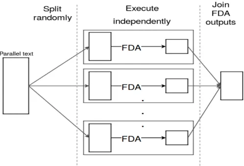
2.8 ParFDA execution diagram . . . 46

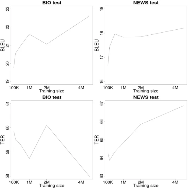
3.1 Results (BLEU and TER) of SMT models trained in different sizes of data. . . 50

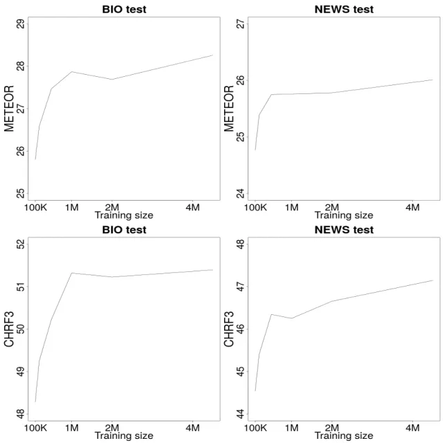
3.2 Results (METEOR and CHRF3) of SMT models trained in different sizes of data. . . 51

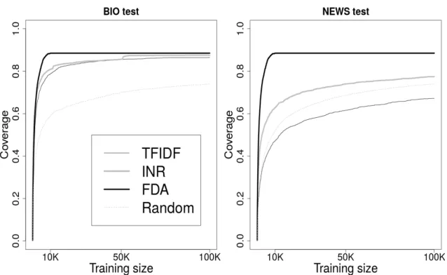
3.3 Coverage of Transductive methods (up to 100K sentences) . . . 55

3.4 Results of TA with different sizes of data for BIO (left) and NEWS (right) test sets. . . 56

4.1 Overview of domain adaptation for NMT. . . 62

4.2 Accuracy and Perplexity of the NMT model in each epoch. . . 67

4.3 Evaluation metrics of the NMT models by epoch. . . 68

4.4 NMT models trained in different sizes of data without BPE (thin line) and with BPE (thick line). . . 70

(8)

4.5 Results of the models trained with TA-selected data. . . 77 5.1 Coverage of the test set using different values of k of INR. . . 89 5.2 Coverage of the test set using different decay factors (values of d in

Equation (2.49)). . . 91 5.3 Coverage of the test set using different decay exponents (values of c

in Equation (2.49)). . . 95 5.4 Distribution of the alignment entropies. . . 100 6.1 Creation of back-translated parallel set. . . 113 6.2 Pipeline of the traditional usage of TAs (left) and pipeline of our

proposal, using the target-side (right). . . 114 6.3 Pipeline of the batch (left) and online (right) processing to obtain

(9)

List of Tables

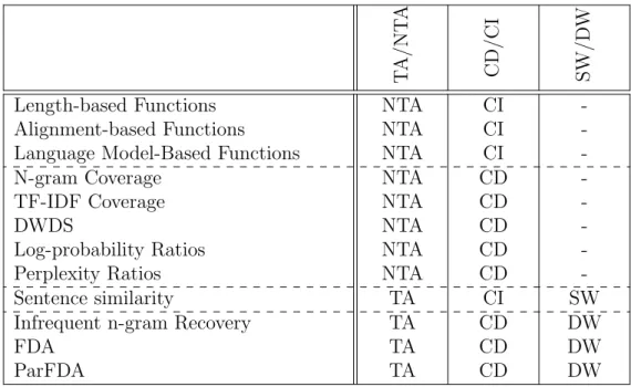
2.1 Classification of data-selection algorithms. . . 38 3.1 Statistics of the data sets. |S| is the number of sentences, |W| the

number of words, and |V| the size of the vocabulary. . . 49 3.2 Results of SMT models built with different sizes of (random) data. . 52 3.3 Percentage of unique sentences in the data retrieved by TFIDF method.

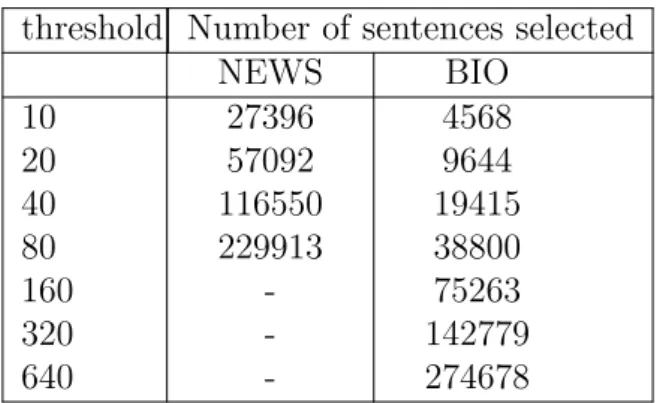
. . . 53 3.4 Number of sentences retrieved by INR using different values of

thresh-old t. . . 54 3.5 SMT models built with different sizes of selected sentences. The

results in bold indicate an improvement over BASE. The asterisk means the improvement is statistically significant at p=0.01. . . 57 3.6 Comparison of outputs produced by SMT models built with

TA-selected sentences. . . 58 4.1 The model using different different merge operations. The results in

bold indicate an improvement over the baseline. An asterisk shows that the improvement is statistically significant at p=0.01 when com-pared towithout BPE, and double asterisks when compared to both

without BPE and 10,000 operations. . . 69 4.2 Results of models built with different sizes of (random) data. . . 71 4.3 Results of the model BASE12 and BASE13 (with and without using

(10)

4.4 NMT models fine-tuned with different sizes of selected data (without BPE). The results in bold indicate an improvement over BASE13. The asterisk means the improvement is statistically significant at p=0.01. . . 75 4.5 NMT models fine-tuned with different sizes of selected data (using

BPE). The results in bold indicate an improvement over BASE13. The asterisk means the improvement is statistically significant at p=0.01. . . 76 4.6 Comparison of outputs produced by models built from scratch. . . . 79 4.7 Comparison of outputs produced by the baseline (general-domain

model on the 13th epoch) and models fine-tuned with selected data. 81 5.1 SMT and NMT models built with different decay of INR. The results

in bold indicate an improvement over default configuration k= 1. . . 90 5.2 SMT and NMT models built with different decay factor of FDA. The

results in bold indicate an improvement over default configurationd= 0.5. The asterisk means the improvement is statistically significant at p=0.01. . . 92 5.3 SMT and NMT models built with different decay exponent of FDA.

The results in bold indicate an improvement over default configu-ration c = 0. The asterisk means the improvement is statistically significant at p=0.01. . . 94 5.4 Results of SMT models trained with data retrieved by INR method

extended with alignment entropies. The results in bold indicate an improvement over default configuration. The asterisk means the im-provement is statistically significant at p=0.01. . . 100

(11)

5.5 Results of SMT models trained with data retrieved by FDA method extended with alignment entropies. The results in bold indicate an improvement over default configuration. The asterisk means the im-provement is statistically significant at p=0.01. . . 101 5.6 Comparison of outputs of the SMT models (100K lines) with data

retrieved from INR and FDA. The configurations shown correspond both to default and extended with alignment entropies. In FDA these are applied as decay factor (DF), decay exponent (DE), or decay factor and exponent (DFE). . . 104 5.7 Results of NMT models trained with data retrieved by INR method

extended with alignment entropies. The results in bold indicate an improvement over default configuration. The asterisk means the im-provement is statistically significant at p=0.01. . . 105 5.8 Results of NMT models trained with data retrieved by FDA method

extended with alignment entropies. The results in bold indicate an improvement over default configuration. The asterisk means the im-provement is statistically significant at p=0.01. . . 106 5.9 Comparison of outputs of the NMT models (100K lines) with data

retrieved from INR and FDA. The configurations shown correspond both to default and extended with alignment entropies. In FDA these are applied as decay factor (DF), decay exponent (DE), or decay factor and exponent (DFE). . . 107 6.1 Results of the models built with different sizes ofIN Rsrc and IN Rtrg

using back-translated data. The results in bold indicate an improve-ment over BASE13. An asterisk shows that the improveimprove-ment is statis-tically significant at p=0.01 when compared to BASE13, and double asterisks when compared to both BASE13 and INR. . . 119

(12)

6.2 Results of the models built with different sizes ofF DAsrc andF DAtrg using back-translated data. The results in bold indicate an improve-ment over BASE13. An asterisk shows that the improveimprove-ment is statis-tically significant at p=0.01 when compared to BASE13, and double asterisks when compared to both BASE13 and FDA. . . 120 6.3 Examples of back-translated sentences . . . 122 6.4 Results of the models built with different sizes ofIN Rsrc and IN Rtrg

using authentic data. The results in bold indicate an improvement over BASE13. An asterisk shows that the improvement is statisti-cally significant at p=0.01 when compared to BASE13, and double asterisks when compared to both BASE13 andα = 1. . . 124 6.5 Results of the models built with different sizes ofF DAsrc andF DAtrg

using authentic data. The results in bold indicate an improvement over BASE13. An asterisk shows that the improvement is statisti-cally significant at p=0.01 when compared to BASE13, and double asterisks when compared to both BASE13 andα = 1. . . 125 6.6 Examples of sentences retrieved by T Asrc and T Atrg. . . 126 6.7 Results of the models built with different sizes of INR-selected hybrid

data. The results in bold indicate an improvement over INR. The asterisk means the improvement is statistically significant at p=0.01. 128 6.8 Results of the models built with different sizes of FDA-selected hybrid

data. The results in bold indicate an improvement over FDA. The asterisk means the improvement is statistically significant at p=0.01. 129 6.9 Number of unique sentences in the target-side of the training data. . 131 6.10 Comparison of outputs of the NMT models (100K lines) with hybrid

data retrieved from INR and FDA following different approaches. . . 132 7.1 Results of the models built with selected data using an in-domain set. 139

(13)

Abbreviations

ANN Artificial Neural Network

BCED Bilingual Cross-Entropy Difference

BLEU Bilingual Evaluation Understudy

BPE Byte Pair Encoding

CBOW Continuous Bag-of-Words Model

CD Context-Dependent

CED Cross-Entropy Difference

CI Context-Independent

CHRF Character n-gram F-score

DW Document-wise

DWDS Density Weighted Diversity Sampling

FDA Feature Decay Algorithms

GRU Gated Recurrent Unit

INR Infrequent N-gram Recovery

LM Language Model

LSTM Long Short-Term Memory

MERT Minimum Error Rate Training

METEOR Metric for Evaluation of Translation with Explicit Ordering

(14)

NLP Natural Language Processing

NTA Non-transductive Algorithms

NMT Neural Machine Translation

PBSMT Phrase-Based Statistical Machine Translation

RNN Recurrent Neural Network

RQ Research Question

SGD Stochastic Gradient Descent

SMT Statistical Machine Translation

SW Sentence-wise

TA Transductive Algorithm

TER Translation Edit Rate

(15)

Improving Transductive Data Selection

Algorithms for Machine Translation

Alberto Poncelas Rodriguez

Abstract

In this work, we study different ways of improving Machine Translation models by using the subset of training data that is the most relevant to the test set. This is achieved by using Transductive Algoritms (TA) for data selection. In particular, we explore two methods: Infrequent N-gram Recovery (INR) and Feature Decay Algo-rithms (FDA). Statistical Machine Translation (SMT) models do not always perform better when more data are used for training. Using these techniques to extract the training sentences leads to a better performance of the models for translating a particular test set than using the complete training dataset.

Neural Machine Translation (NMT) can outperform SMT models, but they re-quire more data to achieve the best performance. In this thesis, we explore how INR and FDA can also be beneficial to improving NMT models with just a fraction of the available data.

On top of that, we propose several improvements for these data-selection methods by exploiting the information on the target side. First, we use the alignment between words in the source and target sides to modify the selection criteria of these methods. Those sentences containing n-grams that are more difficult to translate should be promoted so that more occurrences of thesen-grams are selected. Another extension proposed is to select sentences based not on the test set but on an MT-generated approximated translation (so the target-side of the sentences are considered in the selection criteria). Finally, target-language sentences can be translated into the source-language so that INR and FDA have more candidates to select sentences from.

(16)

Acknowledgments

This thesis has been possible thanks to many people. First, I would like to express my deepest gratitude to Professor Andy Way for his guidance and supervision. I am also thankful for the support and advice of Dr. Gideon Maillette de Buy Wenniger, and Dr. Antonio Toral. In addition, I would like to thank my examiners Dr. Kevin McGuinness and Dr. Will Lewis, and chairperson Dr. Sharon O’Brien.

I embarked on this journey along with my colleagues Pintu Lohar, and Eva Vanmassenhove. For the past four years, we followed a similar path in which we never failed to support each other. My sincere gratitude also goes to my colleagues, and post-docs in ADAPT Centre, particularly Dimitar Shterionov, and Chao-Hong Liu who made this work much easier. Additionally, I want to thank Wichaya Pid-chamook, who has been very helpful.

I will always feel indebted to Emilio Gede´on Ortiz-Garc´ıa for being an inspira-tional mentor and a good friend, and for encouraging me to do a PhD.

Last but not least, I would like to thank my family, particularly my parents Cesar Poncelas Poncelas, and Ana Maria Rodriguez Garcia for their endless support during these years, and indeed for my whole life.

This research has been supported by the ADAPT Centre for Digital Content Technology which is funded under the SFI Research Centres Programme (Grant 13/RC/2106).

(17)

Chapter 1 Introduction

Machine Translation (MT) is a subfield of machine learning that aims to generate the translation of sentences in one language into another language. In order to accomplish this, MT models are built using sentence pairs that are translations of each other. Models learn from these sentences so they can infer the translation of a new, unseen sentence or document.

As the translations produced by the models are typically post-edited by a profes-sional translator, the quality of the generated translations is of crucial importance in order to minimize the amount of human effort.

Although one would think that by adding more sentence pairs, the model pro-duces better translations, this is not necessarily true. It has been shown (Ozdowska and Way, 2009) that Statistical Machine Translation (SMT) models can perform better when trained with less data but in a closer domain to that of the test set. In order to do that, data-selection algorithms aim to retrieve the subset of data that is closer to a particular domain.

For this reason, data-selection techniques play a major role. These techniques aim not only to reduce the size of the models (and the time required for training), but also to identify the data that belong to a particular domain, so the model can be trained with in-domain data.

(18)

1.1 Document-Specific Machine Translation

1.1.1 Domain identification problem

In MT, test sets are usually sampled from a particular set of content (potentially a very large set of content) itself representative from a well-defined source, where that source may be labeled as a ‘domain’. Test data are drawn from news sources (blogs, news websites, etc.) thus representing the ‘News’ domain, or a test data are drawn from medical sources thus representing the ‘medical’ domain, etc.

In some cases determining the domain of the test set can be difficult, and some-times the test set can even belong to multiple domains. Fortunately, the selection of the sentence pairs can be executed without the need for identifying the domain. These data-selection methods that consider the test set as the seed in order to retrieve sentences are those classified as Transductive Algorithms (TAs).

1.1.2 Transductive Learning

TAs operate under a very different paradigm to the standard approaches used in machine learning, which are based on inductive learning. Inductive learning is con-cerned with reasoning from the particular (observed training data) to the general (functions that generalize well to unseen test data). In contrast, transductive learn-ing (Vapnik, 1998) is concerned with the particular to the particular: in our case, from a corpus of annotated MT training data to a specific test set to be trans-lated. Generalization outside this specific test set is not an objective of transductive learning, which can potentially allow transductive methods to outperform inductive models with respect to specific test sets.

As the definition of domain can range from general (e.g. News, Bio, etc) to more particular (such as author profiling), building document-specific MT systems is the most specific example of domain adaptation that might be contemplated.

The use of the test set has been previously investigated in other works. For example, Lu et al. (2007) propose to change the weight of those sentences that are

(19)

similar to the test set. Alternatively, they train several MT model candidates and use the test set to select the most suitable one to generate the translation. Bi¸cici (2011) use the test set to select sentences to make regression based machine translation

computationally more scalable. Lopez (2008) proposeMachine Translation by Patter Matching, where those entries of the phrase table that match the phrases of the test set are retrieved.

1.1.3 Adaptation of Machine Translation Models

A translation company, when they need to translate a new document they use a MT engine that is the most suitable (e.g. trained in the same domain) to generate a translation. However, if at translation time the test set (or the document to be translated) is known, why not benefit from that? An MT model could be adapted to the current document. We propose to postpone part of the training phase of the MT model until the document to be translated is provided, which would minimize the time and human efforts required to post-edit the output of the MT.

The impacts of this view of the MT process are significant, in that two aspects which are central to how MT is done today are radically redefined:

• offline training is reduced or eliminated;

• the notion of poor quality ‘noisy’ data largely disappears;

• the notion of ‘domain’ becomes much more fine-grained and dynamic.

Furthermore, this will completely remove the major barrier and cost associated with MT: personalisation. Today, personalised MT is simply not a possibility, and even for larger institutions, customisation represents a major obstacle.

1.1.4 Cloud-Based Models

As hardware capability continues to improve, we foresee a paradigm shift in the not too distant future where cloud-based models are built on-the-fly in real time

(20)

for translation of specific documents. We envisage that following analysis of the translation requirements of the said document, the best-fitting examples in the entire cloud of translation data are selected as data for training of an MT system built specifically to translate that document. In such a scenario, we expect training time to be fast, as the amount of training data required will be small. In this way, we could even think of such models as disposable; once the specific document has been translated, there is no need to keep the MT system any longer.

Taken together, these improvements have the potential to transform the current MT landscape:

• Speed: translation systems will be built in real time;

• Quality: systems are dynamically adapted on-the-fly, based on the current translation task, and with incremental system-updating in real time during the post-editing process;

• Personalisation: training/customization always takes place online, in real time, to the user’s specific requirements.

These three improvements are tightly interconnected; by permitting personal-isation as a real-time process, we will achieve major improvements in translation quality and speed and considerably enhance the user experience.

1.2 Proposal of the Thesis

While building such an online real-time system-building set-up goes beyond the scope of this thesis, the importance of the optimal selection of the training data becomes paramount. Accordingly, in the context of this thesis, transduction is explored primarily via the use of data selection and data synthesis methods. The key idea is to choose examples from the training corpus that are similar in some way to the test corpus, and then use standard statistical and neural inferential models,

(21)

which will be biased toward performing well on the specific test set. This thesis demonstrates that this can lead to improved performance on the test sets.

We explore the performance1 _{of TAs when used to build German-to-English}

MT models. Initially, we set out to explore the effect of TAs on the prevailing state-of-the-art in MT, namely SMT. More recently, of course, Neural Machine Translation (NMT) approaches have become popular as they can outperform SMT models. NMT models tend to perform better than SMT when larger amounts of data are used for training. Nonetheless, this work also shows that a subset of sentences retrieved by TAs can also be beneficial to improve the performance of NMT models. In addition, we also propose several ways to improve TAs by exploiting informa-tion in the target side. These improvements come from three direcinforma-tions, either by (i) altering the selection criterion; (ii) altering the seed used for selecting sentences (use a translation of the test set instead of the test set); or (iii) generating new candidate sentences that TA can select from.

In sum, the primary focus of study in this thesis is the capability of TAs to restrict the amount of training data needed for the building of a high-quality MT system. However, it would be wrong to conclude that TAs can only be used for this task. Accordingly, at the end of the thesis, we start to consider the extent to which the class of algorithms classified in this thesis as TAs can be used inductively; can they be used to generalise over specific data sets and applied to new ones? Can they be utilised for domain adaptation?

1.3 Research Questions

The Research Question (RQs) we are addressing in this thesis aim to improve the performance of models trained on data selected by TAs. The RQs explored are:

1. RQ1: How can we tailor data-selection algorithms to be most

effec-1_{In this work, performance of a data-selection algorithm is used to refer to the translation}

quality of a model trained with the sentences retrieved by the algorithm, measured with automatic evaluation metrics.

(22)

tive in combination with NMT?

Although the TAs have a good performance in SMT they are yet unexplored in NMT. NMT approaches require larger amounts of data than SMT to achieve their best performances. For this reason, we want to explore whether these models could also benefit from TAs.

2. RQ2: Can word-alignment information be useful for improving

state-of-the-art TAs?

The TAs analyzed in this thesis penalize the n-grams of sentences that have already been selected in order to increase the variability. However, should every n-gram be penalized equally? In every language, there are words or n -grams that are more difficult to be translated and therefore more occurrences are needed in order to learn the proper translation. A way of measuring how complicated is to decide the translation of an n-gram is by computing the alignment entropy, which measures the predictability of the translation by analyzing how the words in then-gram are mapped to the words in the target side.

3. RQ3: Can the use of synthetic sentences improve the performance

of MT models when used in combination with TAs?

Another method to improve the quality of the models is to acquire more candi-dates sentences to selected from. When additional data are not available there is the option of creating sentences artificially. By doing this, we can augment the size of the candidate pool. We want to explore whether using synthetic data alone or in combination with authentic data is more beneficial than using authentic data only.

One limitation of the explored TAs is that they select the sentences based on the n-grams in the source side, ignoring the target-side completely. We propose to use synthetic target-side sentences as the seed of TAs so that the

(23)

selection is also performed considering the target side. By doing this we want to minimize the effect of selecting noisy sentences (sentence pairs that are not accurate translations of each other) and promote selecting the same n-grams in the target side.

1.4 Contributions

In this thesis we use TAs applied in MT and there are several contributions in terms of the exploration and improvements of these methods. Here we present the main contributions of the thesis, but a more detailed list can be found in the introduction of each chapter:

• We perform comparisons of SMT and NMT models that have been trained with different amounts of data.

• We compare different SMT and NMT models using subsets of the training sentences retrieved by TAs.

• We perform an analysis of the performance of different configurations of TAs in SMT and NMT, and explore the impact of changing the values of the parameters of TAs.

• We propose a novel extension for two TAs so that the decay of the n-grams (used to promote the variability) becomes dynamic, and so different n-grams are penalized differently.

• We discuss the disadvantages of selecting parallel sentences with TAs based only in the source side and introduce a novel technique to execute these meth-ods so they select sentences considering the target side instead.

• We investigate how authentic and synthetic training data can work in combi-nation with TAs to build better models. In addition, we propose two ways of

(24)

selecting synthetic data with TAs and how to combine them with the authentic selected-data.

1.5 Outline of the Thesis

This thesis is structured in the following chapters:

• Chapter 2 (Background) introduces some concepts that will be used later on in the thesis. In addition, we describe the two leading MT paradigms Phrase-Based Statistical Machine Translation (PBSMT) and NMT, as the experiments carried out involve building models following these approaches. In addition, we provide an overview of the main data-selection algorithms and describe their main characteristics.

• Chapter 3 (Transductive Algorithms on Statistical Machine

Trans-lation) presents several experiments for a better understanding of PBSMT models. The chapter includes experiments that explore the impact of adding training sentences to build the models. Additionally, in the chapter we inves-tigate the performance when SMT models are built with data selected from TAs. This chapter is also important as we establish the models considered as baselines for SMT in the thesis.

• Chapter 4 (Transductive Algorithms on Neural Machine

Transla-tion) reports the performance of NMT models when trained with data from TAs. This chapter addresses RQ1. We compare NMT models trained with different sizes of either randomly-selected or TA-selected data. We explore two different ways of using selected data in NMT: (i) using it to build models from scratch; and (ii) using it to tune general-domain models. This chapter also helps establish the baselines to be used in our the experiments, as well as describe how NMT models are constructed in the following chapters.

(25)

• Chapter 5 (The Use of Alignment Entropy) presents an analysis of the impact of different configurations when used in SMT and NMT. We propose a method to improve the selection criteria of TAs. In particular, we aim to answer RQ2. We suggest three methods to compute alignment entropies and we evaluate TAs when using these values for their parameters.

• Chapter 6 (The Use of Synthetic Data to Adapt Models)investigates

a set of experiments in which artificial data are involved to answer RQ3. This chapter evaluates the models fine-tuned with synthetic sentences only, as well as in combination with authentic ones.

• Chapter 7 (Conclusions and Future Work) summarizes the work

con-ducted in terms of the RQs proposed in the thesis. Finally, we propose several ways to further explore the techniques proposed in this work.

1.6 Publications

The contents of this thesis are based on work published in peer-reviewed interna-tional conferences. The papers that are the most related are the following:

1. Poncelas, A., de Buy Wenniger, G. M., and Way, A. (2019b). Transductive data-selection algorithms for fine-tuning neural machine translation. In The 8th Workshop on Patent and Scientific Literature Translation (PSLT 2019), Dublin, Ireland

2. Poncelas, A., Maillette de Buy Wenniger, G., and Way, A. (2018b). Feature decay algorithms for neural machine translation. InProceedings of the 21st An-nual Conference of the European Association for Machine Translation, pages 239–248, Alacant, Spain

3. Poncelas, A., Way, A., and Toral, A. (2016). Extending feature decay al-gorithms using alignment entropy. In International Workshop on Future and Emerging Trends in Language Technology, pages 170–182, Seville, Spain. Springer

(26)

4. Poncelas, A., Maillette de Buy Wenniger, G., and Way, A. (2017). Applying n-gram alignment entropy to improve feature decay algorithms. The Prague Bulletin of Mathematical Linguistics, 108(1):245–256

5. Poncelas, A., Shterionov, D., Way, A., de Buy Wenniger, G. M., and Passban, P. (2018c). Investigating backtranslation in neural machine translation. In

21st Annual Conference of the European Association for Machine Translation, pages 249–258, Alacant, Spain

6. Poncelas, A., Popovic, M., Shterionov, D., de Buy Wenniger, G. M., and Way, A. (2019c). Combining SMT and NMT back-translated data for efficient NMT. InProceedings of Recent Advances in Natural Language Processing (RANLP), pages 922–931, Varna, Bulgaria

7. Poncelas, A., de Buy Wenniger, G. M., and Way, A. (2019a). Adaptation of machine translation models with back-translated data using transductive data selection methods. In 20th International Conference on Computational Linguistics and Intelligent Text Processing, La Rochelle, France

8. Poncelas, A., Way, A., and Sarasola, K. (2018d). The ADAPT System Descrip-tion for the IWSLT 2018 Basque to English TranslaDescrip-tion Task. InInternational Workshop on Spoken Language Translation, pages 72–82, Bruges, Belgium 9. Poncelas, A., de Buy Wenniger, G. M., and Way, A. (2018a). Data selection

with feature decay algorithms using an approximated target side. In 15th In-ternational Workshop on Spoken Language Translation (IWSLT 2018), pages 173–180, Bruges, Belgium

10. Poncelas, A. and Way, A. (2019). Selecting Artificially-Generated Sentences for Fine-Tuning Neural Machine Translation. In Proceedings of the 12th In-ternational Conference on Natural Language Generation, Tokyo, Japan In addition to that, there are other papers published in peer-reviewed conferences in the Natural Language Processing (NLP) field that I have co-authored:

(27)

1. Poncelas, A., Sarasola, K., Dowling, M., Way, A., Labaka, G., and Alegria, I. (2019d). Adapting NMT to caption translation in Wikimedia Commons for low-resource languages. In 35th International Conference of the Spanish Society for Natural Language Processing (SEPLN 2019), Bilbao, Spain

2. Vanmassenhove, E., Moryossef, A., Poncelas, A., Way, A., and Shterionov, D. (2019). ABI Neural Ensemble Model for Gender Prediction Adapt Bar-Ilan Submission for the CLIN29 Shared Task on Gender Prediction. InComputational Linguistics of the Netherlands CLIN29, Groningen, The Netherlands (Share task winner paper)

3. Dowling, M., Lynn, T., Poncelas, A., and Way, A. (2018). SMT versus NMT: Preliminary comparisons for Irish. In Technologies for MT of Low Resource Languages (LoResMT 2018), page 12, Boston, USA

4. Silva, C. C., Liu, C.-H., Poncelas, A., and Way, A. (2018). Extracting in-domain training corpora for neural machine translation using data selection methods. In

Proceedings of the Third Conference on Machine Translation: Research Papers, pages 224–231, Brussels, Belgium

5. Liu, C.-H., Moriya, Y., Poncelas, A., and Groves, D. (2017b). IJCNLP-2017 Task 4: Customer Feedback Analysis. In Proceedings of the IJCNLP 2017, Shared Tasks, pages 26–33, Taipei, Taiwan

6. Dzendzik, D., Poncelas, A., Vogel, C., and Liu, Q. (2017). ADAPT centre cone team at IJCNLP-2017 task 5: A similarity-based logistic regression approach to multi-choice question answering in an examinations shared task. InProceedings of the IJCNLP 2017, Shared Tasks, pages 67–72, Taipei, Taiwan (Share task winner paper)

7. Liu, C.-H., Groves, D., Hayakawa, A., Poncelas, A., and Liu, Q. (2017a). Under-standing meanings in multilingual customer feedback. In Proceedings of First

(28)

Workshop on Social Media and User Generated Content Machine Translation (Social MT 2017), Prague, Czech Republic

(29)

Chapter 2 Background

In this chapter, we introduce concepts related to the NLP field that will be used later and provide a background of MT field. In particular, we explain the main state-of-the-art approaches, PBSMT (Koehn et al., 2003) and NMT (Cho et al., 2014; Sutskever et al., 2014), that have been explored in this work.

In addition, as this thesis is related to the data-selection field, in Section 2.5 we summarize the main data-selection techniques. Note that we classify and provide a general overview of major data-selection techniques. Then, in Section 2.5.2 we describe in more detail the transductive methods which are used in the experiments carried out in this thesis.

2.1 Mathematical and NLP Concepts

First, we introduce some mathematical notation and NLP concepts that will be used in this work.

N-gram functions An n-gram is a sequence of n contiguous elements extracted from a longer string. Typically, these elements consist of characters or words. Unless otherwise specified, in this thesis we consider an n-gram to be a sequence of words. We define N grij(s) as the set of n-grams (where i ≤ n ≤ j) in a sentence s. Similarly, we use the notationN grij(D) as the set ofn-grams in a set of sentencesD

(30)

(equivalent to N grij(D) =Ss∈DN grij(s)). For simplification, in the case in which

i= 1, we will indicate only the value of j in the subscript, soN grj(s) =N gr1j(s). Moreover, we use Cs(ngr) as the count of occurrences of an n-gram ngr in a sentence s, and CD(ngr) =

P

s∈DCs(ngr) the number of occurrences of ngr in the set of sentences D.

The probability of the occurrence of an n-gram in a set of sentences D is calcu-lated as in Equation (2.1): PD(ngr) = CD(ngr) P ngri∈N grnn(D) CD(ngri) . (2.1)

We use |s| to express the number of words contained in the sentence s and

words(D) = P

s∈D

|s| as the number of words in the set D.

Parallel Data In the MT field we typically use parallel sentences to build MT models. This data consists of a pairhS, Ti, where S is a set containing sentences in the source language andT a set containing sentences in the target language. These sentences are paired so the i-th sentence si ∈S and ti ∈T are a translation of each other. The pairhS, Tican also be considered a set of unique parallel sentence-pairs

hsi, tii, so we also refer to it as a parallel set.

Following the terminology of the MT field, we also refer to the subsequence of words of a sentences as a phrase ¯s. From a sentence pair hsi, tiiwe can also extract phrase-pairs hf ,¯ ¯ei (where ¯f is a phrase fromsi and ¯e is a phrase from ti). We use

C(S,T)( ¯f ,e¯) for counting the number of sentences in which the phrase ¯f and ¯eoccur

together in hS, Ti.

Entropy Entropy is a measure of the uncertainty. It is used to evaluate the predictability of the outcomes of a random process. The entropy of a random variable

(31)

Equation (2.2):

entropy(X) =− X

xi∈X

P(xi) log(P(xi)). (2.2)

A larger entropy means that the uncertainty is higher and lower entropies indicate that the outcomes are more predictable. If there is only one predictable outcome (P(x1) = 1), then the entropy is 0. The entropy value can be normalized to be in

the range [0,1] when computed as in Equation (2.3):

entropy(X) =− 1

|X|

X

xi∈X

P(xi) log(P(xi)). (2.3)

TF-IDF Term Frequency–Inverse Document Frequency (TF-IDF) (Salton and

Yang, 1973) is a statistic that indicates how relevant a word is for a document in relation to a set of documents. The weight of a term is higher if it is frequent in a document d, but it is also penalized if is also frequent in the other documents of the collection D.

The TF-IDF value of word wk in a document d ∈ D is computed as in Equa-tion (2.4):

tfidf(wk, d, D) =Cd(wk) log(idf(wk, D)) (2.4) where idfk is the inverse document frequency (IDF). This measures the inverse of the frequency of thek-th term in the set of all documentsD, computed as idf(wk) =

|D|

|D_wk| whereDwk is the set of documents containing wk.

TF-IDF is often used as a distance metric between two documents. A document can be seen as a vector d where each element dk is tf idf(wk, d, D). The TF-IDF distance of two vector of two documentsd(1) andd(2) is defined as the cosine distance

between the two vectors computed as in Equation (2.5):

disttf idf(d(1),d(2)) = cos(d(1),d(2)) =

d(1)·d(2)

|d(1)||d(2)|

(32)

Language models Language Models (LMs) are models that measure the fluency of a sentence, i.e. how likely the sentence is to have been produced by a native speaker of the language. N-gram LMs are based on statistics that indicate how likely words are to follow each other.

However, Equation (2.1) is not useful to estimate the probability as ngr may not be found in D (which is likely if the sequence is too long). Therefore, n-gram LMs split this process (smaller statistics) using the chain rule and aim to predict one word at a time as in Equation (2.6):

PLM(w1, w2, ..., wl−1, wl) =P(w1)P(w2|w1)...P(wl|w1, w2, ..., wl−1). (2.6)

The terms of Equation (2.6) compute the probability of a word conditioned to the sequence of all previous words. Following the Markov assumption, each term

P(wi|w1...wi−1) is approximated as in Equation (2.7):

P(wi|w1, w2, ..., wi−1)≈P(wi|wi−h, w2, ..., wi−1) (2.7)

where, instead of considering all the previous word of the sequence, only the previous

hwords are considered. We callhthe order of the LM. Each term of Equation (2.7) is computed as in Equation (2.8):

PLMd(wi|wi−h, ..., wi−1) =

CD(wi−h, ..., wi)

CD(wi−h, ..., wi−1)

. (2.8)

In order to evaluate an LM, two metrics are typically used: cross-entropy and perplexity. This metrics estimate how well an LM can predict a sequence of words

s. The first metric, cross-entropy, is the average log probability of the words in s

computed as in Equation (2.9): HLMd(s) =− 1 |s| |s| X i=1

(33)

The other metric, perplexity, is a transformation of cross-entropy as in Equa-tion (2.10):

P PLMd(s) = 2

H_LMd(s)_. _(2.10)

2.2 Statistical Machine Translation

SMT is the MT paradigm in which the translation problem is considered as a sta-tistical optimization problem.

The noisy channel model is a framework of communication where a message is sent from the source to a receiver through a channel which causes the message to suffer a distortion. SMT is based on this framework as it assumes a sentence f

in a source language is transformed into a sentence e in the target language when transmitted through the noisy channel. The goal is to infer the translated sentence

e from f with the highest probability as in Equation (2.11):

e∗ = arg max e

P(e|f) (2.11)

which following Bayes’ theorem, can be expressed as in Equation (2.12) (noisy chan-nel model):

P(e|f)∝P(f|e)P(e) (2.12)

where we observe two main components:

• P(f|e), translation model probability, which measures adequacy, i.e how much of the meaning is preserved in the translation. This model is built based on bilingual data.

• P(e), language model probability, which measures fluency, i.e. how likely the translation is to have been produced by a native speaker of that language. This model is built based on monolingual (target-side) data.

(34)

2.2.1 Word-Based Statistical Machine Translation

Word-based SMT (Brown et al., 1993) is the statistical translation approach that uses words as atomic translation units. It introduced the concept of word alignment, a function defining one-to-one and many-to-one mappings between words of the sentence pairs.

Given a sentence f = (f1, ..., fls) in the source language and a sentence e =

(e1, ..., elt) in the target language, the alignment function a maps each word ej in

the target-side to a wordfi in the source side along with the translation probability. The most popular tools for word alignments are GIZA++ (Och and Ney, 2003) and its variation FastAlign alignment model (Dyer et al., 2013) which introduces a diagonal tension λ. This parameter measures the overall correspondence of word order and an efficient re-estimation of the parameters that makes it around 10 times faster than GIZA++ while still obtaining comparable quality.

2.2.2 Phrase-Based Statistical Machine Translation

PBSMT models (Koehn et al., 2003) may be considered to be an improvement over word-based SMT models. These models use phrases as atomic units for translation (as opposed to individual words). This approach is better able to capture contextual information. Phrases from a source and a target sentence are paired so that every word of the phrase in one side is aligned to a word present in the phrase of the other side or a hNULLitoken (but not to words outside the phrase).

The phrase pairs are gathered along with their translation scores in a structure called a phrase-table, which will be used in the decoding step (when translating a document) as a look-up dictionary, for selecting a translation of a phrase of the test set.

The decision to select a phrase pair is based mainly on three components: (i) a translation model (scores of the phrase-table), (ii) a reordering model, and (iii) a LM:

(35)

• Translation model: It provides the translation probabilities of a phrase pair (an entry of the phrase table). Commonly 4 scores are computed: “inverse phrase translation probability” (φ(f|e)), “inverse lexical weighting” (lex(f|e)), “direct phrase translation probability” (φ(e|f)) and “direct lexical weighting” (lex(e|f))

– Translation probability: It indicates the probability of a phrase to be the translation of another phrase computed as in Equation (2.13):

φ( ¯f|e¯) = _PC(S,T)( ¯f ,e¯)

¯

fi

C(S,T)( ¯fi,e¯)

(2.13)

where ¯f and ¯e are the source and target phrase pairs, respectively.

– Lexical weighting: This is computed in order to avoid the problem of phrases that do not provide reliable probability estimations (e.g. low-frequency phrases). It measures how well the words in the phrases trans-late to each other (Koehn et al., 2003) computed as in Equation (2.14):

pw( ¯f|e, a¯ ) = l Y i=1 1 {j|(i, j)∈a} X ∀(i,j)∈a w(fi|ej) (2.14)

wherew(fi|ej) is the lexical weighting defined as in Equation (2.15):

w(fi|ej) =

C(S,T)(fi, ej)

P

f0C(S,T)(f0, ej)

(2.15)

wheref0 are the words in the source language aligned toej

• Reordering model: Introduced by Tillmann (2004), this is the model that handles the orientation of a phrase based on the previous adjacent phrase. Koehn et al. (2005) estimates the probability of three different orientations for a phrase: monotone (how likely the phrase follows the previous one), swap (how likely is swapped with the previous one) and discontinuous (how likely it is not to be connected to the previous one).

(36)

• LM: An LM models the fluency of the output of the translation computing the probability of a sequence of words as in Equation (2.8):

These scores computed are combined in a weighted logarithmic sum (known as the log-linear model) as in Equation (2.16):

p(x) = exp n

X

i=1

λihi(x). (2.16)

As we see in Equation (2.16), the feature functions are weighted according to

λi. After computing the feature functions, the optimal value of each λi needs to be found. The process of finding appropriate values of λi is known as tuning.

One popular method for tuning is Minimum Error Rate Training (MERT) (Och, 2003). MERT uses a development set, a set of parallel sentences not included in the training data, to estimate the optimal weights. In order to estimate them, first initial random values are set, and then several runs are executed (until convergence). In each iteration:

1. Translations of the sentences in thedev set are produced and the error of the

n-best sentences (using the reference translations) are computed.

2. Each parameter is optimized individually (fixing the values of the other pa-rameters).

2.2.3 Moses Toolkit

The PBSMT tool we use in this work is the Moses Toolkit (Koehn et al., 2007). This tool takes a set of parallel sentences and a language model as input and trains an SMT system. It computes the models explained in Section 2.2.2 and produces a file, moses.ini, that contains the features as shown in Listing 2.1.

The first part of themoses.inifile contains the paths to the components explained in Section 2.2.2 (translation model, lexical reordering and language model) and other

(37)

UnknownWordPenalty WordPenalty P h r a s e P e n a l t y P h r a s e D i c t i o n a r y M e m o r y name=T r a n s l a t i o n M o d e l 0 num−f e a t u r e s =4 p a t h=/p a t h / t o / p h r a s e−t a b l e . g z i n p u t−f a c t o r =0 o u t p u t−f a c t o r =0 L e x i c a l R e o r d e r i n g name=L e x i c a l R e o r d e r i n g 0 num−f e a t u r e s =6 t y p e=wbe−msd−b i d i r e c t i o n a l−f e−a l l f f i n p u t−f a c t o r =0 o u t p u t−f a c t o r =0 p a t h=/p a t h / t o / r e o r d e r i n g−t a b l e . wbe−msd−b i d i r e c t i o n a l−f e . g z D i s t o r t i o n KENLM l a z y k e n =0 name=LM0 f a c t o r =0 p a t h=/p a t h / t o /LM o r d e r =8 L e x i c a l R e o r d e r i n g 0= 0 . 0 8 9 9 0 2 3 0 . 0 5 8 9 2 5 3 0 . 0 4 5 6 7 9 6 0 . 0 8 7 9 3 9 7 0 . 0 0 0 1 2 2 1 0 6 0 . 1 3 5 8 9 6 D i s t o r t i o n 0= 0 . 0 2 9 4 9 9 3 LM0= 6 . 1 5 0 9 7 e−05 WordPenalty0= −0 . 0 1 6 4 7 1 3 P h r a s e P e n a l t y 0= −0 .2 91 07 T r a n s l a t i o n M o d e l 0= 0 . 0 0 0 1 1 9 4 8 1 0 . 0 2 0 7 1 7 3 0 . 2 2 2 7 9 9 −0 . 0 0 0 7 9 7 1 8 6 UnknownWordPenalty0= 1

Listing 2.1: Extraction of moses.ini file using default configuration of Moses

wenn w i r | | | when we | | | 0 . 2 0 0 6 0 . 1 7 7 2 0 . 1 1 0 0 . 1 5 5 1 | | | 0−0 1−1 | | | 6 4 8 1 1 7 7 1 3 0 | | | | | |

wenn w i r | | | when | | | 0 . 0 0 0 6 0 1 5 0 . 0 0 0 7 4 2 8 0 . 0 0 5 1 0 . 1 9 9 5 | | | 0−0 | | | 9 9 7 4 1 1 7 7 6 | | | | | |

wenn w i r | | | w h e n e v e r we | | | 0 . 1 8 1 8 0 . 1 8 5 1 0 . 0 0 3 3 9 8 0 . 0 0 3 3 7 6 | | | 0−0 1−1 | | | 22 1 1 7 7 4 | | | | | |

wenn w i r | | | w h e r e we | | | 0 . 0 0 3 8 7 5 0 . 0 1 1 4 8 0 . 0 0 0 8 4 9 6 0 . 0 0 5 9 2 7 | | | 0−0 1−1 | | | 2 5 8 1 1 7 7 1 | | | | | |

wenn w i r | | | w h i l e we | | | 0 . 0 1 4 9 2 0 . 0 0 9 1 5 1 0 . 0 0 0 8 5 0 . 0 0 2 9 2 6 | | | 0−0 1−1 | | | 67 1 1 7 7 1 | | | | | |

Listing 2.2: Extraction of phrase table file

features such as word and phrase penalty (so the translations are not too long or too short), unknown word penalty and distortion (Brown et al., 1993).

The second part of the file contains the weights of the features (λi values in Equation (2.11)). In Listing 2.1 we show the values after tuning.

We can observe in the first part of themoses.inifile (Listing 2.1) that the trans-lation model (PhraseDictionaryMemory), reordering model (LexicalReordering) and language model (LM) indicate the files where these models are stored. Note that the translation model and reordering model files have been created by Moses, but the language model is created separately and then provided to Moses at training time.

The translation model is stored in a file called phrase table. We show an ex-traction in Listing 2.2. This file contain five columns (the separator of the table is “|||”)

1. Phrase in the source side.

2. Phrase in the target side: the phrase in the target side language that is paired with the source side phrase.

(38)

3. Translation model features: The four probabilities explained in Section 2.2.2 in this order: inverse phrase translation probability, inverse lexical weighting, direct phrase translation probability, and direct lexical weighting. We describe the first row of Listing 2.2 as an example of how they are computed:

• Inverse phrase translation probability (φ(f|e)): this is computed as in Equation (2.13). The counts of occurrences of the phrases are shown in column 5 (“when we” occurs 648 times, “wenn wir” and “when we” occur together 130 times). Therefore the inverse phrase translation probability is 0.2006 = 130/648.

• Inverse lexical weighting (lex(f|e)): this is computed as in Equation (2.14). The individual lexical weighting is stored in a file called lex.e2f created by Moses. In this file we find the values of lexical weighting for the words in the phrases, in the rows wenn when 0.2658521 and wir we 0.6666557. Therefore the inverse lexical weighting is 0.1772 = 0.2658521·0.6666557.

• Direct phrase translation probability (φ(e|f)): this is computed as in Equation 2.13. “wenn wir” occurs 1177 times, “wenn wir” and “ when we” occur together 130 times. Therefore the direct phrase translation probability is 0.110 = 130/1177.

• Direct lexical weighting (lex(e|f)): this is computed as in Equation (2.14). The individual lexical weighting is stored in a file calledlex.f2e which con-tains the rows when wenn 0.1995174 and we wir 0.7773823. Therefore the direct lexical weighting is 0.1551 = 0.1995174·0.7773823.

4. Alignments: How words of the source and target side are aligned individually. For example, in the last row, the pairh“wenn wir , when we”i, “0-0” indicate that the 0-th word in the source side word (“wenn”) is aligned to the 0-th target-side word (“when”).

(39)

wenn w i r | | | when | | | 0 . 2 0 0 0 0 0 0 . 0 6 6 6 6 7 0 . 7 3 3 3 3 3 0 . 3 3 3 3 3 3 0 . 0 6 6 6 6 7 0 . 6 0 0 0 0 0 wenn w i r | | | w h e n e v e r we | | | 0 . 2 7 2 7 2 7 0 . 0 9 0 9 0 9 0 . 6 3 6 3 6 4 0 . 0 9 0 9 0 9 0 . 0 9 0 9 0 9 0 . 8 1 8 1 8 2 wenn w i r | | | w h e r e we | | | 0 . 2 0 0 0 0 0 0 . 2 0 0 0 0 0 0 . 6 0 0 0 0 0 0 . 2 0 0 0 0 0 0 . 2 0 0 0 0 0 0 . 6 0 0 0 0 0 wenn w i r | | | w h i l e we | | | 0 . 2 0 0 0 0 0 0 . 2 0 0 0 0 0 0 . 6 0 0 0 0 0 0 . 2 0 0 0 0 0 0 . 2 0 0 0 0 0 0 . 6 0 0 0 0 0

Listing 2.3: Reordering table

phrase counts, source and target intersection count. For example, in the first example “wenn wir , when we”, there are 1177 occurrences of “wenn wir”, and 648 occurrences of “when we”. The phrases “wenn wir” and “ when we” occur together 130 times,

The reordering model is also stored in a separate file. We show an extraction in Listing 2.3. This file contain three columns (the separator of this table is also “|||”):

1. Phrase in the source side.

2. Phrase in the target side. The phrase in the target side language that is paired with the source side phrase.

3. Orientation probabilities: Six probabilities in two sets indicating the orienta-tion (monotone, swap and discontinuous) in both direcorienta-tions (left-to-right and right-to-left), with each set of probability summing to 1.

2.3 Neural Machine Translation

More recently, NMT approaches have become more popular than SMT. Instead of using phrases as translation units like in PBSMT models, in NMT approaches, the sentences are encoded as vectors. These vectors are inputs (and outputs) of a network whose nodes models a function. In the training process, the parameters of the functions are adjusted so the returned vector encodes the sentence corresponding to the translation of the input.

(40)

2.3.1 Word Vector Models

A straightforward technique to encode a word as a vector is via the so called one-hot vector encoding. Assuming a vocabulary of size V we can encode the i-th word in the vocabulary as vector v ∈ _R|V| _{with 1 in the i-th position and 0 in the other} positions.

However, this is a sparse representation in which there is no relationship between the words. For example, given this representation, the distance between two related words such as football and basketball is the same as football and plane, even though, the last two are semantically more different than the first pair. Word embeddings aim to find the position of the words in the vector space so that similar words are grouped close to one another.

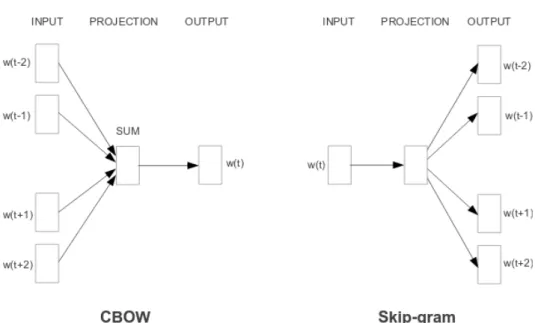
In Mikolov et al. (2013) two methods for computing word embeddings are pro-posed (Figure 2.1):

• Continuous Bag-of-Words Model (CBOW): This model tries to predict a word

wtgiven the context. This means that the previous sequence of words (vectors

wt−1...wt−i) and the following sequence of words (vectors wt+1...wt+i)) are used as input to a neural network architecture.

• Skip-gram Model: The objective is to predict the context words given a word

wt. It improves the quality of the resulting word vectors, but it also increases the computational complexity (Mikolov et al., 2013).

The main benefit of these representations is the generalization it brings. Similar words will have similar vectors and so the distance between them will be small (as opposed to one-hot vectors where all vectors are equidistant from one another). Another benefit is that we can represent the words using a lower dimensional vector.

2.3.2 Artificial Neural Networks

Inspired by biological neural networks, Artificial Neural Network (ANN) are com-puting systems that are made up of interconnected processing elements (called

(41)

per-Figure 2.1: CBOW and Skip-gram Word Embedding Models. (Mikolov et al., 2013)

ceptrons).

The networks receive a series of inputs x1, x2...xdx (which can be expressed as

elements of a vector x∈Rdx_{). These inputs are processed by perceptrons and then}

a series of outputs y1, y2, ...ydy (which can be seen as elements of a vector y∈ R

dy₎

are produced.

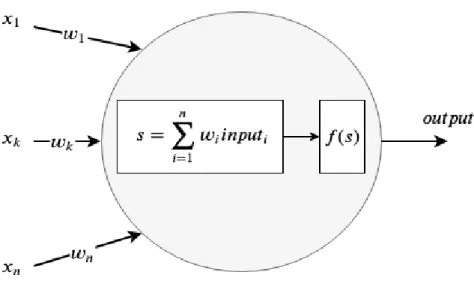
In Figure 2.2 we see an example of a simple perceptron. The perceptron applies a weighted sum of the inputs (for simplification purposes we omit the bias), activation function and then feeds forward the results.

An example of a simple network is the multilayer perceptron in which perceptrons are structured in layers, as in Figure 2.3, that are classified in three types:

• Input Layer: A layer in which the perceptrons receive the input and feed it to the next layer.

• Hidden layer (one or several): A layer in which perceptrons gather the inputs from the previous layer (which can be the input layer or another hidden layer), perform the computations and feed the result to the next layer.

(42)

Figure 2.2: Example of a perceptron.

provide the final output of the function that the network is approximating.

Figure 2.3: Example of an ANN.

As perceptrons are structured on layers, each layer can be modeled as in Equa-tion (2.17):

h=f(Wihx) (2.17)

wherexis the output of the previous layer (each element in the vector is the output of one perceptron) or the input vector. f(x) is a non-linear activation function such

(43)

as the f(x) = ₍₁₊1_e−x₎ (also known as sigmoid function or σ) or f(x) = tanh(x).

The matrix Wih ∈ R|h|×|x| is composed of the individual weights wij of the link connecting the output of the j-th perceptron of the previous layer (i.e. xj) with the i-th perceptron in the hiden layer (hi).

The output layer is modeled as in Equation (2.18):

y=g(Whoh) (2.18)

g(x) is also a non-linear activation function. In the case of using the ANN as classification function a popular function of g(x) is the softmax function g(xi) =

exi

P

jexi

. This will produce an output y that encodes the probabilities so each yi encodes the probability of the input belonging to the i-th class (which implies that

P

yi = 1).

The purpose of an ANN is to approximate a function φ(x). When a certain inputxis provided to the input layer of the ANN, the information is propagated to the next hidden layer. Each hidden layer performs the computations (modeled in Equation (2.17)) and emit the signal to the next layer. Eventually, the output layer will provide an output y. This process is known as forward propagation. After exe-cuting the forward propagation, the errorφ(x)−y is computed. Then, the gradient of the error with respect to the weights Wof the different layers is calculated. This process is known as backpropagation as it is computed backward from the output layer to the input layer. Finally, using an optimizer such as Stochastic Gradient Descent (SGD), the error can be reduced by changing the weights in the direction of the gradient.

ANNs are trained using a set of pairs (x, φ(x)). After adapting the weights by performing several iterations of forward propagation and backpropagation, the outputs of the ANN converge to an approximation of the function φ(x).

(44)

2.3.3 Recurrent Neural Networks

Recurrent Neural Networks (RNNs) are ANNs that form directed cyclic graphs. Having this structure allows the RNN to compute a sequence of vectors instead of a single vector.

Each vector xt in the sequence (x1,x2, ...xTx) is sequentially processed (Figure

2.4). At the step of processingxt, the information of the previous output vectorht−1

is also gathered. Then, the hidden state ht and the output yt are produced. The diagram presented in Figure 2.4 can be unfolded to take time out of the equation as in Figure 2.5.

Figure 2.4: Example of an RNN.

Figure 2.5: Example of an unfolded RNN.

(45)

previous hidden layer ht−1), Equation (2.17) is extended as in Equation (2.19):

ht =f(Wihxt+Uihht−1) (2.19)

where Wih and Uih are the weight matrices to be adjusted during training of the RNN.

RNNs obtain the information of the previous hidden state ht−1 when

process-ing xt, which implicitly contains the information of the previous elements of the sequence. However, the long-distance dependencies are more difficult to learn the more the bigger the gap between xt and a previous element xt−k is.

In order to solve this long-distance dependency problem Long Short-Term Mem-ories (LSTM) (Hochreiter and Schmidhuber, 1997) was proposed as a variation of RNNs. As the experiments involving RNNs executed in this work consist of LSTM, in Section 2.3.4 we explain them in more detail. Later, alternatives to LSTM such as Gated Recurrent Units (GRUs) (Cho et al., 2014) were proposed. Nonetheless, it has been shown that both approaches have similar performance (Chung et al., 2014).

2.3.4 Long Short-Term Memory

LSTM is an improvement over the general RNN architecture. The particularity of LSTM is that it has two inputs (ht−1 and ct−1) and two outputs (ht and ct), where the signal ct contains the long-distance information. As presented in Figure 2.6,

ct encodes the signal ct−1 with minor updates. This causes the value of ct (at the iteration t) to retain information from the previous steps.

The process that is executed in an LSTM cell in Figure 2.6 can be broadly described via three main steps:

1. Forget step: In this step, it is decided whether the information of the memory cell ct−1 should be kept or forgotten. This is measured by the forget gateftas

(46)

Figure 2.6: Diagram of LSTM.

in Equation (2.20).

ft =σ(Wfxt+Ufht−1). (2.20)

2. Update step: In this step, it is decided what should be stored in the memory state. In this step the candidate values ˜ctare created and the input gate layer

it, as Equation (2.21) and Equation (2.22), respectively:

˜

ct =tanh(Wcxt+Ucht−1) (2.21)

it =σ(Wixt+Uiht−1). (2.22)

3. Output creation step: During the last step, the outputsctandhtare produced.

• ctis a combination of how much is forgotten of the previousct−1 and how

much it is updated with new values. It is computed as in Equation (2.23):

(47)

• ht combines the cell statect (normalized with tanh function to make the values be in the range (−1,1)) with the output gate ot which modulates how much memory content is considered.

ht=ottanh(ct) (2.24)

where ot is the output gate. It depends on the current output and the previous hidden state as in Equation (2.25).

ot=σ(Woxt+Uoht−1). (2.25)

2.3.5 Encoder-Decoder Architecture

An RNN transforms a sequence of vectors into another target sequence, but both sequences are of the same length. The Encoder-Decoder framework (Cho et al., 2014; Sutskever et al., 2014) is an architecture introduced to solve this problem.

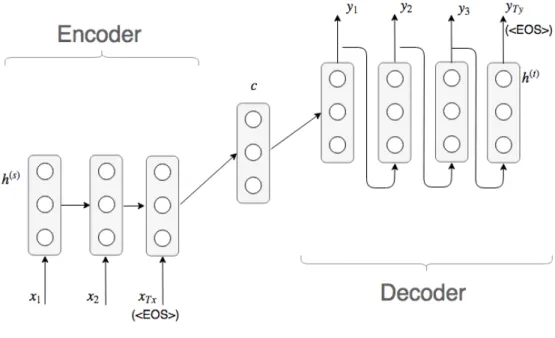
In Figure 2.7 we can find the structure of a basic Encoder-Decoder framework. It consists of two RNNs (an encoder and a decoder) that transform a sequence

X = (x1,x2, ...,xTx) into another sequence Y = (y1,y2, ...,yTy), where the sequence

can differ in length.

• Encoder: The encoder converts the sequence (x1,x2, ...,xTx) into a context

vector c that summarizes the sentence. This vector c is constructed by con-sidering the hidden vectorsh(_ts_x) (wheretx ∈[1, Tx]) of the encoder (we useh

(s)

i to denote the i-th vector of the sequence generated by the encoder andh(_it) to denote the i-th vector generated by the decoder). When the last element of the sequence hEOSi is encoded, the context vector c is sent to the decoder.

• Decoder: The decoder performs the inverse process of the encoder. Given the context vectorcit produces the vectorsh(_t_yt) (until the elementhEOSiis found) that are decoded as the targets sequence of vectors. (y1,y2, ...,yTy).

(48)

Figure 2.7: Encoder-Decoder model

2.3.6 Attention Model

The problem of the encoder-decoder framework is that it encodes the whole sequence as a single vector. However, especially for the longer sequences, it may lead to an information loss. This has a negative impact on the decoder has it only has access to the vectorc to generate the sequence of sentences.

The Attention Model (Bahdanau et al., 2014) was introduced to solve this prob-lem. Using this mechanism, instead of using a single fixed context vectorcto encode the input sequence, a context vector for each output time step ct is created. This helps the decoder to identify the parts in the input sequence that are relevant in order to generate the subsequent words. The vector ct is computed as the weighted sum of h(s) _{as in Equation (2.26):} ct = Tx X i=1 αtih (s) i (2.26)

where the weights αti indicate how much attention should yt pay to each h

(s)

i (i.e. how muchyt is related to the element xi of the input sequence) and it is computed

(49)

as a softmax function as shown in Equation (2.27). αti = exp(a(h(_t−t)₁,h(_is))) PTx k=1exp(a(h (t) t−1,h (s) k )) (2.27) where the function a is the alignment model. The alignment model we use in this work is computed as in Equation (2.28):

a(h(_t−t)₁,h_i(s)) =h(_t−t)₁Wah

(s)

i (2.28)

whereWais a weight matrix that is trained jointly with the other parts of the NMT model.

2.4 Translation Performance Evaluation Metrics

Translation performance evaluation metrics are used to evaluate the translation quality of the output of a translation model. These metrics compare the hypothesis (the output of the system) against a reference and determine how similar they are. In this work we are measuring the translated outputs using the following metrics:

• Bilingual Evaluation Understudy (BLEU) (Papineni et al., 2002) uses match-ing n-grams between the hypothesis and reference to give a quality score. The score is in the range [0,1] but often is given as a percentage measure.

The BLEU score is computed as in Equation (2.29):

BLEU(hyp, ref) =BP ·exp

N

X

n=1

1

N logP Rn (2.29)

where N typically has a value of 4, and P Rn is the precision computed as the number ofn-grams in common (between the hypothesis and the reference) divided by the number of n-grams in the hypothesis. However, the number of common n-grams should be limited to the maximum number of instances in the reference. For example, for the reference sentence “the airport” the

(50)

unigram precision of the hypothesis “the the” would be 2₂ = 1. For this reason the precision is clipped, and is computed as in Equation (2.30):

P Rn =

X

ngr∈N grnn(hyp)

min(Chyp(ngr), Cref(ngr))

X

ngr∈N grnn(hyp)

Chyp(ngr)

(2.30)

which would cause the unigram precision in the example to be 1₂.

BP is the brevity penalty defined as BP = min(1, e1−

|ref|

|hyp|_{). It is introduced}

to penalize those candidates that are shorter than the reference (those longer than reference are already penalized by the precision measure).

• Translation Edit Rate (TER) (Snover et al., 2006) computes the minimum number of edits required to make the hypothesis match the reference. The edits include insertion, deletion or substitution of single words and shifts of word sequences. It is computed as in (2.31):

T ER= # edits

average # of reference words. (2.31)

• Metric for Evaluation of Translation with Explicit Ordering (METEOR) (Baner-jee and Lavie, 2005) provides a score matching words and phrases of the hy-pothesis and reference. There are three types of match:

– exact: two unigrams match if they are exactly the same,

– stem: two unigrams match if they are the same after they have been stemmed,

– synonymy: two unigrams match if they are synonyms of each other. All the words in the candidate must match at most one word in the reference. The number of matches is used to compute the precisionP = #match_|hyp| and recall

(51)

R= #match_|ref| to compute the METEOR score as in Equation (2.32):

M ET EOR= 10P R

R+ 9P(1−P enalty) (2.32)

where P enalty = 0.5#chunk_#match

3

and #chunk indicates the minimum number of chunks in which all the words in the hypothesis can be grouped. A chunk is the sequence of words (in adjacent positions) in the hypothesis that are also mapped to a sequence of words in the reference.

Unlike the other evaluation metrics we are presenting here, this is a language-dependent evaluation metric as the unigrams are aligned using stemmer and synonym tables.

• Charactern-gram F-score (CHRF) (Popovic, 2015): It is an evaluation metric that operates at the character level. It computes the F-score as in Equa-tion (2.33):

CHRF β = (1 +β2) CHRP ·CHRR

β2 _·_CHRP ₊_CHRR (2.33)

where:

– CHRP: Percentage of n-grams (character level) in the hypothesis which are in the reference (precision).

– CHRF: Percentage of n-grams (character level) in the reference which are also present in the hypothesis (recall).

– β: is a hyperparameter that assigns β times more importance to recall than to precision. In this work we are computing the value where β = 3, which Popovic (2015) demonstrated to be correlated with human judg-ment.

Improving transductive data selection algorithms for machine translation

Improving Transductive Data

Selection Algorithms for Machine

Translation

Alberto Poncelas Rodriguez

B.Sc., M.Sc.

Doctor of Philosophy (Ph.D.)

Dublin City University

School of Computing

Supervisors:

Prof. Andy Way, Dr. Gideon Maillette de Buy Wenniger

Contents

List of Figures

List of Tables

Abbreviations

Improving Transductive Data Selection

Algorithms for Machine Translation

Alberto Poncelas Rodriguez

Abstract

Acknowledgments

Chapter 1

Introduction

1.1

Document-Specific Machine Translation

1.1.1

Domain identification problem

1.1.2

Transductive Learning

1.1.3

Adaptation of Machine Translation Models

1.1.4

Cloud-Based Models

1.2

Proposal of the Thesis

1.3

Research Questions

1.4

Contributions

1.5

Outline of the Thesis

1.6

Publications

Chapter 2

Background

2.1

Mathematical and NLP Concepts

2.2

Statistical Machine Translation

2.2.1

Word-Based Statistical Machine Translation

2.2.2

Phrase-Based Statistical Machine Translation

2.2.3

Moses Toolkit

2.3

Neural Machine Translation

2.3.1

Word Vector Models

2.3.2

Artificial Neural Networks

2.3.3

Recurrent Neural Networks

2.3.4

Long Short-Term Memory

2.3.5

Encoder-Decoder Architecture

2.3.6

Attention Model

2.4

Translation Performance Evaluation Metrics