Lattice determination of Sigma-Lambda mixing

arXiv:1411.7665v2 [hep-lat] 16 Apr 2015

ADP-14-36/T895 DESY 14-220 Edinburgh 2014/20 Liverpool LTH 1027 April 15, 2015

A lattice determination of Sigma – Lambda

mixing

R. Horsley

_{, J. Najjar}

_{, Y. Nakamura}

_{, H. Perlt}

_,

D. Pleiter

, P. E. L. Rakow

, G. Schierholz

,

A. Schiller

, H. St¨

uben

and J. M. Zanotti

– QCDSF-UKQCD Collaboration –

a _{School of Physics and Astronomy, University of Edinburgh,}

Edinburgh EH9 3FD, UK

b _{Institut f¨ur Theoretische Physik, Universit¨at Regensburg,}

93040 Regensburg, Germany

c _{RIKEN Advanced Institute for Computational Science,}

Kobe, Hyogo 650-0047, Japan

d_{Institut f¨ur Theoretische Physik, Universit¨at Leipzig,}

04109 Leipzig, Germany

e _{J¨ulich Supercomputer Centre, Forschungszentrum J¨ulich,}

52425 J¨ulich, Germany

f _{Theoretical Physics Division, Department of Mathematical Sciences,}

University of Liverpool, Liverpool L69 3BX, UK

g _{Deutsches Elektronen-Synchrotron DESY,}

22603 Hamburg, Germany

h _{Regionales Rechenzentrum, Universit¨at Hamburg,}

20146 Hamburg, Germany

i _{CSSM, Department of Physics, University of Adelaide,}

Adelaide SA 5005, Australia

Abstract

between between these states. We describe the formalism necessary to de-termine the QCD mixing matrix and hence find the mixing angle and mass splitting between the Sigma and Lambda particles due to QCD effects.

1

Introduction

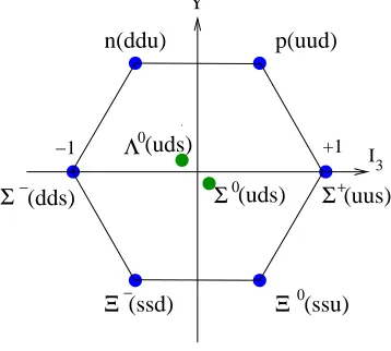
Mass breaking effects in hadron octets (and decuplets) are mainly due to a com-bination of quark mass differences and electromagnetic effects, but can also some-times have an additional component due to mixing between the hadron states. In this article we consider the baryon octet as shown in Fig. 1 where the spin 1 2

baryons are plotted in theI3–Y plane. The particles on the (outer) ring, namely

+

0 −

0

+1 −1

Ξ

Σ

p(uud)

Ξ

(uds)

I

3

Λ0(uds)

Σ−(dds)

n(ddu)

(ssd) (ssu)

Σ (uus)

Y

Figure 1: The lowest octet for the spin 1₂ baryons plotted in the I3–Y plane.

the n(ddu), p(uud), Σ−_{(dds), Σ}+_{(uus) and Ξ}−_{(ssd), Ξ}0_{(ssu) all consist of}

com-binations of aabquarks (where we use the notation of denoting a quark, q, by a,

b, . . .which can be the up u, down d or strange s quark). a here are the flavour doubly represented quarks, whileb is the flavour singly represented quark. Foru

–d quark mass differences these isospin breaking effects are small. Examples for the lowest baryon octet are the n₋p, Σ−_−Σ+ _{and Ξ}− _−Ξ0 _{mass differences.}

In [1] we investigated the hadronic QCD contribution to these isospin breaking splittings using lattice techniques. In this article we extend these results to the Σ0_−Λ0 _{baryon octet masses. The method developed here for the Σ}0_−Λ0 _mass

splitting will automatically encompass the other splittings.

The Σ0 _{and Λ}0 _masses1 _{are accurately known; from the Particle Data Group}

[2] we have

M_Σexp0 = 1.192642(24) GeV, M

exp

Λ0 = 1.115683(6) GeV, (1) 1_{We use Σ to stand for the unmixed Sigma particle (pure isospin 1) and Σ}0 _{to denote the}

giving a mass splitting of

(MΣ0 −M_Λ0)exp = 76.959(23) MeV. (2) This is very much larger than the other mass splittings mentioned above, which are all of the order of a few MeV. It is also more complicated than other mass splittings as while both baryons have the same quark content, namely u, d, s, most of the mass difference is due to their different wave functions. However there will also be additional mixing between these states. This will be apparent when we later consider Σ(ll′_{s) and Λ(ll}′_{s) where l and l}′ _{are distinct quarks, but} mass degenerate, which already has this large mass splitting.

Understanding how this mixing works will be useful for understanding other mixing cases, such asη₋η′_{orω−φmeson mixing, for which lattice simulations are} considerably more difficult as there are computationally intensive disconnected terms in the correlation function to consider, [3, 4, 5, 6]. In these latter cases a state at the centre of the octet (the pure ‘η8’ octet state) mixes with a further

singlet state, ‘η1’. The case here of Σ0 −Λ0 mixing is a little different as the

particles have the same quantum numbers but now lie in the same octet (as shown in Fig. 1). In Fig. 2 we sketch the expected situation for the Lambda and

M2 B

Λ Σ

mu+md−2ms

Λ

Σ

H

L

Figure 2: A sketch of the heavy,H, and light,L, baryon (masses)2_againstm

u+md−

2ms for fixed mu−md. The mass splitting between the Sigma and Lambda masses

in the isospin limit (mu =md) is given by the difference between the (red) circles; if mu 6= md then there is an additional mass difference due to mixing, the filled (blue)

circles. Further explanation of the figure is given in the text.

Sigma hadrons, plotting M2

B against mu +md−2ms. The lines represent lines

(blue) lines are formu−md6= 0. The central point is the quark mass symmetric

point, when all quark masses are the same, when there is no difference between the Lambda and Sigma masses. In the isospin limit, when mu = md 6= ms we

sit at the points denoted by an open (red) circle. The mass splitting between the Sigma and Lambda particles is given by the vertical difference between these points.

However ifmu 6=md then we have mixing between the ‘Lambda’ and ‘Sigma’

particles, as also depicted in the figure by (blue) lines. The physical Σ0 _{and Λ}0

masses are now given by the (blue) filled circles. We see that there is then an additional mass splitting.

As can also be seen from the figure, depending on the numerical values of the quark masses, the physical Σ0 _{and Λ}0 _{masses can have a larger or smaller}

component of the original ‘Σ’ and ‘Λ’ particles. To avoid confusion we shall call in future the lower branch the ‘Light’ orLbranch with associated massML, while

the upper is the ‘Heavy’ orH branch with mass MH. For example in the isospin

limit mu =md≡ml we have

MH = (

MΣ ml < ms

MΛ ml > ms

, ML= (

MΛ ml< ms

MΣ ml> ms

. (3) At the physical point, denoted by a ∗_{, we set}

MΣ0 =M_H∗ , M_Λ0 =M_L∗. (4) In the following we denote the pure octet, i.e. unmixed Σ and Λ mass states, by the Hermitian matrix

M2

ΣΣ MΣΛ2

M2

ΛΣ MΛΛ2

!

, (5)

while the mixed mass states will be denoted by M2

H, ML2. We determine the

mixing angle,θΣΛ, which rotates eq. (5) with rotation matrix

R= cosθΣΛ e

iφΣΛsinθ

ΣΛ

−e−iφΣΛ_sinθ

ΣΛ cosθΣΛ

!

, (6)

to the diagonal form

M2

H 0

0 ML2 !

, (7)

whereφΣΛis the phase. Note that for the general symmetry arguments used here

mixing of roughly the same order of magnitude as isospin breaking effects. Thus we consider ‘pure’ QCD effects only. The method also applies to mixing ofJP ₌

1 2

+

baryons in the singly charmed sector. For csu(or csd) baryons the hadronic mixing will be far larger than electromagnetic effects.

Previous determinations of Σ – Λ mixing include using the quark model, e.g. [7], chiral perturbation theory, e.g. [8] and from ‘sum rule’ methods, e.g. [9, 10]. The plan of this article is as follows. In the next section, section 2, we first discuss in more detail the calculational strategy that we employ here. In partic-ular as summarised in section 2.3, and discussed further in Appendices A and B we make a SU(3) flavour expansion about a point with degenerate mass u, d

ands quarks. Section 3 then gives the Σ – Λ mass mixing expansion up to NLO (i.e. next-to-leading order or quadratic in the quark masses). We have actually computed the expansion to NNLO (i.e. next-next-to-leading order), but as we only use these to help to estimate systematic errors, the complete expansions are relegated to Appendix C. We also show numerical simulations with two mass degenerate sea quark masses as sufficient to determine the expansion coefficients also for the non-degenerate quark mass case. In section 4 we modify the expan-sion, to consider ratios, rather than lattice or scale dependent quantities. Some comments on matrix elements are given in section 5. Our numerical simulations are then detailed in section 6 and correlation functions and determination of the expansion coefficients are given in sections 6.1 and 6.2, together with results for mass degenerate quarks. Finally our results and discussion are given in section 7.

2

The

SU

(3)

flavour expansion

2.1

Mass matrix symmetries

When all three quarks have the same mass, an SU(3) transformation U on the quark fields is a symmetry of the action; it leaves the quark mass matrix, _M unchanged. We, however, are more interested in what happens in the case of unequal quark masses

M=



 

mu 0 0

0 md 0

0 0 ms 



 , (8)

when we make an SU(3) transformation

M′ _=UMU†_{. (9)}

This is easiest to see if the transformation U is simply a permutation. For example, if we interchangemd andmswe still get the same set of baryon masses,

(see Fig. 1); all that changes is the names we give them. In this case, Mn and

MΞ0 would be interchanged, as wouldM_p and M_Ξ+ and so on. A rotation of the quark mass matrix simply leads to a corresponding rotation of the baryon mass matrix, M,

M(U_MU†) =UM(_M)U†. (10) TheU matrices in eq. (9) belong to a 3_×3 matrix representation ofSU(3), while the U matrices in eq. (10) belong to an 8_×8 representation of the same group.

We can see from eq. (10) that the mass matrix and the (mass matrix)2 _both

transform in the same way

M2 _→(UMU†)(UMU†) =UM2U† (11) (where, as always, M2 _{is shorthand for MM). Therefore, as far as symmetry}

arguments go, it makes no difference whether we discuss the hadron mass matrix, or the mass-squared matrix. Note also that we can see from eq. (11) that the eigenvectors of M and of M2 _{are the same.}

We consider in future theSU(3) flavour breaking expansion ofM2 _{rather than}

M, [8]. Thus we set

M2 =



             

M2

n 0 0 0 0 0 0 0

0 M2

p 0 0 0 0 0 0

0 0 M2

Σ− 0 0 0 0 0

0 0 0 M2

ΣΣ MΣΛ2 0 0 0

0 0 0 M2

ΛΣ MΛΛ2 0 0 0

0 0 0 0 0 M2

Σ+ 0 0 0 0 0 0 0 0 M2

Ξ− 0

0 0 0 0 0 0 0 M2

Ξ0



             

. (12)

The reason is that as in [1] we have found again that better numerical fits in the quark mass range considered are obtained using the hadron mass matrix squared.

In Appendix A an explicit example for the transformation u_↔d is given.

2.2

The

Σ

–

Λ

mass matrix

2.2.1 Derivation

The SU(3) flavour expansion classifies mass polynomials according to the S3

permutation group and theSU(3) flavour group. S3 is the symmetry group of an

equilateral triangle, C3v. This group has 3 irreducible representations, [11], two

different singlets,A1 and A2 and a doublet E, with elements E+ and E−. Some

n p Σ− _{Σ Λ Σ}+ _Ξ− _Ξ0 _S

3 SU(3)

1 1 1 1 1 1 1 1 A1 1

−1 ₋1 0 0 0 0 1 1 E+ ₈

a

−1 1 ₋2 0 0 2 ₋1 1 E− ₈

a

1 1 ₋2 ₋2 2 ₋2 1 1 E+ ₈

b

−1 1 0 mix 0 1 ₋1 E− ₈

b

1 1 1 ₋3 ₋3 1 1 1 A1 27

1 1 ₋2 3 ₋3 ₋2 1 1 E+ ₂₇

−1 1 0 mix 0 1 ₋1 E− ₂₇

1 ₋1 ₋1 0 0 1 1 ₋1 A2 10,10

0 0 0 mix 0 0 0 A2 10,10

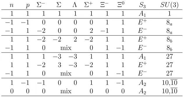
Table 1: Mass matrix contributions for octet baryons, classified by permutation and

SU(3) symmetry. (See Table V in [12].)

In [12] we classified the 10 matrices (Ni, i= 1, . . . ,10) which can contribute

to the octet baryon mass matrix eq. (12) according to their permutation, S3 and

SU(3) symmetry, see Table 1. The compact notation of Table 1 gives just the diagonal elements (the rows/columns being denoted byn, p, . . .). From Table 1 we see that seven of the matrices are diagonal, they can be read off directly from the table. For example the first row gives the 8_×8 matrix: diag(1,1,1,1,1,1,1,1). The table also contains three matrices which mix the Σ and Λ, the fifth, eighth rows which mix at the quadratic quark mass level and the tenth row which mixes with the cubic terms. All the matrices are explicitly listed in Appendix B. Thus we write

M2 =

10

X

i=1

KiNi, (13)

whereKi are some functions of the quark masses (to be determined).

We now need the three non-diagonal matrices in full. From Appendix B they are N5, N8 and N10. We thus have

E− ₈

b



             

−1 0 0 0 0 0 0 0 0 1 0 0 0 0 0 0 0 0 0 0 0 0 0 0 0 0 0 0 _√2

3 0 0 0

0 0 0 _√2

3 0 0 0 0

0 0 0 0 0 0 0 0 0 0 0 0 0 0 1 0 0 0 0 0 0 0 0 ₋1



             

E− ₂₇               

−1 0 0 0 0 0 0 0 0 1 0 0 0 0 0 0 0 0 0 0 0 0 0 0 0 0 0 0 ₋√3 0 0 0 0 0 0 ₋√3 0 0 0 0 0 0 0 0 0 0 0 0 0 0 0 0 0 0 1 0 0 0 0 0 0 0 0 ₋1

               (15)

A2 10,10

              

0 0 0 0 0 0 0 0 0 0 0 0 0 0 0 0 0 0 0 0 0 0 0 0 0 0 0 0 ₋i 0 0 0 0 0 0 i 0 0 0 0 0 0 0 0 0 0 0 0 0 0 0 0 0 0 0 0 0 0 0 0 0 0 0 0

               . (16)

We are now ready to write down the general form of the Σ₋Λ mass matrix. From Table 1 we see that the A1 terms always make equal contributions to the

Σ and Λ; and theE+ _{terms always make opposite contributions to the Σ and Λ.}

From eqs. (14) and (15) we see thatE−_{terms contribute a real symmetric mixing} term, and from eq. (16) that A2 terms contribute an imaginary, antisymmetric

mixing. The allowed form of the Σ₋Λ mass matrix eq. (5) is therefore

M2

ΣΣ MΣΛ2

M2

ΛΣ MΛΛ2

!

(17)

= PA1

1 0 0 1

!

+PE+ 1 0 0 ₋1

!

+PE−

0 1 1 0

!

+PA2

0 ₋i i 0

!

,

wherePG means a function of the quark masses with the symmetryGunder the

S3 permutation group.

We can also give a permutation argument for eq. (17). The Σ and Λ form an

E representation of the permutation group, with the pure Σ even under u _↔ d

and the Λ odd. If mu 6=md there will be mixing between these states. Because

the Σ and Λ have opposite behaviours under u _↔d exchange, the mass matrix for the Σ₋Λ system must have the behaviour

even odd odd even

!

, (18)

under the operation u _↔ d. The possible symmetries of the terms in the mass matrix are given by

The A1 and the E+ member of the E doublet are even under u ↔ d, so they

must be responsible for the diagonal part of the mass matrix. The mixing terms in the mass matrix are odd, so they must come fromE− _{and A}

2 expressions.

From the above discussion we note that the formalism includes the no–mixing case when mu =md; we simply set

PE− = 0, P_A2 = 0, (20)

and the upper component of eq. (17), now in a diagonal form, gives the degenerate mass of the Sigma baryons: Σ _≡ (Σ−_,Σ0_,Σ+_{) (which upon interchanging the}

quarks also gives the other baryon masses on the outer ring N _≡ (n, p), Ξ _≡ (Ξ−_,Ξ0_{)), while the lower component gives Λ.}

2.2.2 Diagonalisation

We now diagonalise the 2_×2 (mass matrix)2 _{of eq. (17) giving eigenvalues}

MH2 = PA1 +

q

P2

E+ +P_E2−+PA22

ML2 = PA1 −

q

P2

E+ +P_E2−+PA22, (21) while if the eigenvectors are written as

eH =

cosθΣΛ

e−iφΣΛ_sinθ

ΣΛ

!

, eL= −

eiφΣΛsinθ

ΣΛ

cosθΣΛ

!

, (22) (cf eq. (6)) we have

tan 2θΣΛ =

q

P2

E−+PA22

PE+

, tanφΣΛ=

PA2

PE−

, (23) for the mixing angle,θΣΛ, and phase, φΣΛ. Note that eq. (21) trivially gives the

H and Lmasses and also the mass difference MH −ML.

Alternatively thePGcoefficients have some nice links to theH andLmasses.

PA1 gives the average (mass)

2

1 2

MH2 +ML2

=PA1, (24) while the other three coefficients contribute symmetrically to the splitting of the two states

1 2

MH2 −ML2

=qP2

2.3

The

SU

(3)

flavour expansion

Our strategy, as discussed in detail in [12] is to start from a point in the quark mass plane with all three sea quark masses equal,

mu =md =ms≡m0, (26)

and extrapolate towards the physical point, denoted by a star, ∗_{, keeping the} average sea quark mass

¯

m = 1

3(mu+md+ms) (27)

constant at the valuem0. As we approach the physical point, theu anddquarks

become lighter, but the s quark becomes heavier. Pions are decreasing in mass, but K and η increase in mass as we approach the physical point. Keeping ¯m

constant greatly reduces the number of mass polynomials which can occur in Taylor expansions of physical quantities within an SU(3) multiplet. As we are expanding about the symmetric point, it is useful to introduce the notation

δmq ≡mq−m ,¯ q=u, d, s . (28)

Note that it follows from the definition that

δmu+δmd+δms = 0, (29)

so we could eliminate one of theδmqs. However we often keep all three terms as

we can then write some expressions in a more obviously symmetrical form. We can also generalise theSU(3) flavour expansion to the case when the mass of the valence quarks can be different to the mass of the sea quarks, i.e. we leave the ‘unitary line’. We call this the ‘partially quenched’ or PQ case. To do this we introduce

δµq =µq−m ,¯ q =u, d, s , (30)

where µq is the valence quark mass. In distinction to the sea quarks there is no

restriction of the form eq. (29) on the values of the valence quark masses. We give our results in this slightly more general case and then specialise to the unitary case δµq →δmq and then to the physical point δmq →δm∗q. This generalisation

will prove to be useful for the numerical determination of the SU(3) expansion coefficients.

In the following we give SU(3) flavour symmetry breaking expansions up to cubic terms in the quark’s mass, i.e. to O(δµ3

q) (in both the sea and valence

Polynomial S3 SU(3)

1 A1 1

δµu+δµd+δµs A1 1

2δµs−δµu−δµd E+ 8

δµu−δµd E− 8

(δµu+δµd+δµs)2 A1 1

(δµu+δµd+δµs)(2δµs−δµu−δµd) E+ 8

(δµu+δµd+δµs)(δµu−δµd) E− 8

(δµs−δµu)2+ (δµs−δµd)2+ (δµu−δµd)2 A1 1 27

(δµs−δµu)2+ (δµs−δµd)2−2(δµu−δµd)2 E+ 8 27

(δµs−δµu)2−(δµs−δµd)2 E− 8 27

δm2

u+δm2d+δm2s A1 1 27

Table 2: All the quark mass polynomials needed for partially quenched masses, clas-sified by symmetry properties. The table includes entries up to O(δµ2_q). (Table XIV of [12].)

3

The

Σ

–

Λ

mixing mass formula

3.1

Expansion of the

P

coefficients

We now return to the evaluation of the Σ – Λ mass matrix as discussed in sec-tion 2.2 and demand that under all SU(3) transformations

M → M′ _=UMU† _{⇔ M}2₍

M′_{) =UM}2₍

M)U†_{. (31)}

Physically there is no change, just a relabelling of the states. For example md↔

ms is equivalent to relabelling Mn ↔MΞ0, . . .

The most general form of the partially quenched octet baryon mass matrix, for 1 + 1 + 1 valence and sea quarks, up to order δµ3

q, in the case where ¯m is

held constant can now be determined. In Appendix B we illustrate explicitly the computation to leading order (LO) of the SU(3) flavour expansion and Σ – Λ mixing. We find that the coefficients2 _{in the Σ – Λ mixing matrix, eq. (17), are}

PA1 = M

2

0 + 3A1δµ¯

+1

6B0(δm 2

u+δm2d+δm2s) +B1(δµ2u+δµ2d+δµ2s)

+1

4(B3+B4)

h

(δµs−δµu)2+ (δµs−δµd)2+ (δµu−δµd)2 i

+C0δmuδmdδms+ 3C1δµ¯(δm2u +δm

2

d+δm

2

s)

−4(C5+C7)δµuδµdδµs+ 1₂Q1(δµs+δµu)(δµs+δµd)(δµu+δµd)

2_{Note thatA}

1andA2are used both for theS3representation and the expansion coefficient.

+27₄Q2(δµs−δµ¯)(δµu−δµ¯)(δµd−δµ¯),

PE+ = 3

2A2(δµs−δµ¯)

+1₂B2(2δµ2s−δµ2u−δµ2d)

+1

4(B3−B4)

h

(δµs−δµu)2+ (δµs−δµd)2−2(δµu−δµd)2 i

+3

2C2(δµs−δµ¯)(δm 2

u+δm

2

d+δm

2

s) + 6(C3−C4)(δµs−δµ¯)δµ¯2

+1 6Q3

h

(δµs−δµu)2+ (δµs−δµd)2−2(δµu−δµd)2 i

δµ¯ +1

8Q4(δµs−δµ¯)(δµ 2

u+δµ2d+δµs2−3δµ¯2),

PE− =

√

3

2 A2(δµd−δµu)

+√₂3B2(δµ2d−δµ2u) +

√

3

4 (B3−B4)

h

(δµs−δµd)2−(δµs−δµu)2 i

+√₂3C2(δµd−δµu)(δm2u+δm2d+δm2s) + 2

√

3(C3−C4)(δµd−δµu)δµ¯2

+₈√1

3Q4(δµd−δµu)(δµ 2

u+δµ2d+δµ2s−3δµ¯2)

−√23Q3(δµd−δµu)(δµs−δµ¯)δµ ,¯

PA2 = C9(δµs−δµu)(δµs−δµd)(δµu−δµd), (32) where

Q1 ≡ 2C3+C5+C7

Q2 ≡ C5−C6+C7+C8

Q3 ≡ 4(C3−C4) + 3(C5−C7)

Q4 ≡ 2(C3−C4) + 3(C5−C7)−9(C6+C8), (33)

and

δµ¯_≡ 1₃(δµu+δµd+δµs). (34)

We can check that all the polynomials that occur here are polynomials of the ap-propriate symmetry from Table 2 (i.e. Table XIV of [12]), or linear combinations of those polynomials. For example forE+ _{we have written}

1 2(2δµ

2

s−δµ2u−δµ2d) = 13(δµu+δµd+δµs)(2δµs−δµu−δµd) (35)

+1₆((δµs−δµu)2+ (δµs−δµd)2−2(δµu−δµd)2).

PE+ and P_E− form a doublet, i.e. they are related by S₃ symmetry, and involve

the same parameters.

Using these expansions eqs. (21) and (23) now give the H and L masses, together with the mixing angle θΣΛ and phase φΣΛ. Note that in the unitary

limit δµq→δmq these expressions simplify greatly

PA1 = M

2

0 + 121(2B0+ 12B1+ 9B3+ 9B4)(δm 2

u+δm2d+δm2s)

PE+ = 3

2A2δms+ 1

8(2B2+ 3B3−3B4)

h

3δm2s−(δmu −δmd)2 i

+1₈(12C2+Q4)δms(δm2u+δm2d+δm2s)

PE− =

√

3

2 A2(δmd−δmu) +

√

3

4 (2B2+ 3B3−3B4)δms(δmu−δmd)

+ 1

8√3(12C2+Q4)(δmu−δmd)(δm 2

u +δm

2

d+δm

2

s)

PA2 = C9(δms−δmu)(δms−δmd)(δmu −δmd). (36)

3.2

Mass formulae, octet hadrons,

2 + 1

case

Let us now consider the equal mass valence up and down quark limit, i.e.

δµu =δµd≡δµl; (37)

then PE− = 0 = PA2 (and PA1, PE+ simplify) which means that θΣΛ = 0, i.e. there is no Σ – Λ mixing, eq. (17) is already diagonal and so

M_Σ2 =PA1 +PE+, M

2

Λ =PA1−PE+, (38) with3 _A

2 >0.

However as there is now no mixing then the mass formula must also auto-matically describe the Σ+_{, Σ}− _{and hence all the ‘outer’ baryons, with flavour} structure aab, eq. (12). Replacingδµl by δµa and δµs by δµb we find

M_Σ2(aab) _≡ M_Σ2(aa′_b)

= M₀2+A1(2δµa+δµb) +A2(δµb−δµa)

+1

6B0(δm 2

u+δm

2

d+δm

2

s)

+B1(2δµ2a+δµ

2

b) +B2(δµ2b −δµ

2

a) +B3(δµb−δµa)2

+C0δmuδmdδms

+[C1(2δµa+δµb) +C2(δµb−δµa)](δm2u +δm2d+δm2s)

+C3(δµa+δµb)3+C4(δµa+δµb)2(δµa−δµb)

+C5(δµa+δµb)(δµa−δµb)2+C6(δµa−δµb)3. (39)

The notation used here is meant to indicate thata,a′ _(anda′′_{) are distinct quarks} (in the baryon wave function), but are mass degenerate, i.e. µa = µa′ (= µ_a′′)4

This agrees with our previous results in [1] and [12] (and justifies the notation for the expansion coefficients of eq. (32)). The valence flavour structure of eq. (39)

3_{From eq. (32) we have P}

E+ = 3₂A2(δµs−δµ¯) +. . . =A2(δµs−δµl) +. . .. From eq. (3) (and Fig. 2), generalising to PQ quarks, eq. (30), we see that withA2 >0 if δµl < δµs then

MH describes MΣ while ifδµl > δµs then ML describes MΣ. Hence MΣ2 is always given by

PA1+PE+. SimilarlyM

2

Λ is given byPA1−PE+.

4_{It should be clear from the context whether we are referring to the Sigma particle or}

then describes the broken isospin case ofp_≡Σ(uud),n _≡Σ(ddu), Σ+ _≡Σ(uus),

Σ− _{≡ Σ(dds), and Ξ}0 _{= Σ(ssu), Ξ}− _{= Σ(ssd) as well as the isospin degenerate} Σ0 _≡Σ(ll′_{s). Furthermore now that we have cubic terms present, the} Coleman-Glashow mass relation [13] is violated,

Mn2−Mp2−MΣ2−+M_Σ2+ +M_Ξ2−−M_Ξ20

= 2(C4−3C6)(δµs−δµu)(δµs−δµd)(δµd−δµu) (40)

(compare with eq. (38) in [12]).

At the cubic level we have four new coefficients C3, C4, C5, C6 involving the

valence quarks alone, and three new coefficients C0, C1, C2 which involve the sea

quark masses, and which drop out for calculations on the symmetric background,

δmq = 0. Eq. (39) assumes that ¯m, the average sea quark mass, is held constant.

A large number of additional terms appear if that constraint is relaxed. If we work on single background all the sea quark terms can be absorbed into the valence parameters; the B0 and C0 terms can be absorbed into M02; C1 and C2

can be absorbed intoA1 and A2 respectively.

Useful for numerical simulations is to take mass degenerateuanddsea quarks, so we have 2 + 1 flavours rather than 1 + 1 + 1 in the generation of configurations

δmu =δmd ≡δml, (41)

which (together with eq. (29)) is equivalent to the replacements

δm2l ↔ 16(δm 2

u+δm2d+δm2s), δm3l ↔ −12δmuδmdδms, (42)

in eq. (32) for PG, G=A1, E+,E−, A2.

Similarly we can write down the mass of the octet Lambda baryon as

M2

Λ(aa′b) = M02+A1(2δµa+δµb)−A2(δµb−δµa)

+1₆B0(δm2u+δm2d+δm2s)

+B1(2δµ2a+δµ2b)−B2(δµ2b −δµ2a) +B4(δµb−δµa)2

+C0δmuδmdδms

+[C1(2δµa+δµb)−C2(δµb−δµa)](δm2u+δm2d+δm2s)

+C3(δµa+δµb)3 + (C4−2C3)(δµa+δµb)2(δµb−δµa)

+C7(δµa+δµb)(δµb−δµa)2+C8(δµb−δµa)3. (43)

If all three quark masses are the same then all the masses become degenerate,

MΣ2(aaa′′)≡MΣ2(aa′a′′)≡MΛ2(aa′a′′). (44)

mass MΣ = MΣ(lls) = MΣ(ll′s) and Xis, Ξ−,Ξ0 ≡ Ξ(ssl) with mass MΞ =

MΣ(ssl), but can also be extended to incorporate the fictitious baryon, Ns(sss′′)

with massMΣ(sss′′). Furthermore the expansion in eq. (43) also incorporates not

only the Lambda, Λ _≡ Λ(ll′_{s) with mass M}

Λ = MΛ(ll′s), but can be extended

to the fictitious baryon Λ2sl(ss′l) with massMΛ(ss′l). For three mass degenerate

valence quarks, we see that this mass formula reduces to the previous formula

MΛ(ll′l′′) =MΣ(lll′′) and MΛ(ss′s′′) = MΣ(sss′′).

The Λ mass formula involves several parametersB4,C7 and C8 which do not

appear in the other baryon masses. We can understand why some terms in M2 Λ

are constrained by the other hadron masses, while others are independent. The partially quenched quantities

(XN2)P Q ≡ ₃1(MN2 +MΣ2 +MΞ2), (XΛ2)P Q≡ 12(M 2

Λ+MΣ2) (45)

agree with each other exactly if δµs = δµl (unbroken valence SU(3), eq. (44)).

The quantity (X2

Λ)P Q −(XN2)P Q is a 27-plet, so it should be O((δµs−δµl)2) if

valence SU(3) is broken. Therefore any terms in M2

Λ which survive, or vanish

more slowly than (δµs−δµl)2, asδµs →δµl are constrained by the other baryon

masses; any terms which vanish like (δµs−δµl)2 or faster can have new

indepen-dent coefficients unconnected to the other baryon masses. The B4, C7 and C8

terms are the only terms in M2

Λ which vanish fast enough as δµs →δµl to evade

this (X2

Λ)P Q→(XN2)P Q constraint, as from eqs. (39) and (43) we find5

(X_Λ2)PQ₋(XN2)PQ = ₆1(3B4−B3)(δµs−δµl)2

+₁₈1(3C7−C5−9C6+ 9C8)(δµs−δµl)3

+1

9(3C7−6C3−C5)(δµs+ 2δµl)(δµs−δµl)

2_{. (46)}

At the O(δµ2

q) level all the coefficients M02, Ai, Bi occur in eqs. (39), (43),

and so can be found from a 2 + 1 flavour partially quenched calculation. (The coefficients are functions of ¯m, and so will not change from a 1 + 1 + 1 simulation to a 2 + 1 simulation provided that ¯m is held constant.) This will no longer hold at O(δµ3

q), to find PA2 we would need to measure the other A2 mass combina-tion, which is the Coleman–Glashow violacombina-tion, eq. (40) or eq. (38) of [12], which requires 1 + 1 + 1 valence quarks and a more general expansion than given in eqs. (39) and (43), so we have introduced a new coefficient, C9, here.

5 _{For completeness, we also give here the result for (X}2 Λ)

PQ

−(X2 N)

PQ _{in the full 1 + 1 + 1}

case, generalising eq. (46),

(XΛ2) PQ

−(XN2) PQ

= 1

4(3B4−B3)(δµ 2 u+δµ

2 d+δµ

2 s−3δµ¯

2

) +3

4(3C7−C5−9C6+ 9C8)(δµs−δµ¯)(δµu−δµ¯)(δµd−δµ¯)

+1

2(3C7−6C3−C5)(δµ 2 u+δµ

2 d+δµ

2 s−3δµ¯

2_{)δµ ,¯}

4

Scale independent quantities

4.1

Ratios

We now restrict ourselves to giving results to NLO (which will be sufficient for our numerical determinations). For completeness the full NNLO expressions are given in Appendix C.

Numerically it is advantageous to consider scale independent quantities, as previously discussed and used in [1, 12]. As stated in section 2.3 flavour blind (or singlet) quantities are suitable to form both scale independent mass ratios and to determine the scale. We denote these quantities generically by XS. One

useful type can be considered as the ‘centre of mass’ of the multiplet. Thus for the baryon octet, one possibility is

XN2 = 16(M 2

p +Mn2 +MΣ2+ +M_Σ2−+M_Ξ20 +M_Ξ2−)

= M2

0 + (16B0+B1+B3)(δm 2

u+δm2d+δm2s). (47)

At the physical point this has the value [2]

XNexp = 1.1610 GeV. (48)

As discussed in [12] flavour blind quantities, due to the vanishing of the linear

δmq terms, (see eq. (47)) remain almost constant as we approach the physical

point, so aN = (aNXN)/XNexp determines the lattice spacing aN(κ0), [12]. (We

have introduced theN subscript as we are using XN to set the scale.)

We shall in future consider for the baryon octet the dimensionless ratios

˜

M2 _≡ M

2

X2

N

, . . . , (49)

and we wish to rewrite eq. (21) in the form

˜

M2

H = P˜A1+

q

˜

P2

E+ + ˜P_E2−+ ˜PA22 ˜

ML2 = P˜A1−

q

˜

P2

E+ + ˜P_E2−+ ˜PA22, (50) and eq. (23) as

tan 2θΣΛ =

q

˜

P2

E−+ ˜PA22 ˜

PE+

, tanφΣΛ=

˜

PA2 ˜

PE−

, (51) where

PG →P˜G =

PG

X2

N

This can be achieved by defining

˜

Ai =

Ai

M2 0

, B˜i =

Bi

M2 0

, (53)

together with the replacement

B0 →B˜0 = −6

B1+B3

M2 0

=₋6( ˜B1+ ˜B3). (54)

The ˜PG, G=A1,E+, E−, A2 scale independent flavourSU(3) expansion

coeffi-cients are then given to NLO by

˜

PA1 = 1 + 3 ˜A1δµ¯

+1₆B˜0(δm2u+δm2d+δms2) + ˜B1(δµ2a+δµ2b +δµ2c)

+1₄( ˜B3+ ˜B4)

h

(δµc−δµa)2+ (δµc−δµb)2+ (δµa−δµb)2 i

,

˜

PE+ = 3

2A˜2(δµc−δµ¯)

+1₂B˜2(2δµc2−δµ2a−δµ2b)

+1₄( ˜B3−B˜4)

h

(δµc−δµa)2 + (δµc−δµb)2−2(δµa−δµb)2 i

,

˜

PE− =

√

3

2 A˜2(δµb−δµa)

+√₂3B˜2(δµ2b −δµ2a) +

√

3

4 ( ˜B3−B˜4)

h

(δµc −δµb)2 −(δµc −δµa)2 i

,

˜

PA2 = 0, (55)

and

δµ¯_≡ 1

3(δµa+δµb+δµc) (56)

(where we have written the more generalδµa, δµb, δµc rather than the previous

δµu,δµd,δµs respectively).

Similarly the changes to the baryon masses for mass degenerate up and down quarks are relatively simple. For completeness we give the scale independent flavour SU(3) expansions

˜

MΣ2(aab) = 1 + ˜A1(2δµa+δµb) + ˜A2(δµb −δµa) (57)

+ ˜B0δm2l + ˜B1(2δµ2a+δµ2b) + ˜B2(δµ2b −δµ2a) + ˜B3(δµb−δµa)2,

and

˜

M_Λ2(aa′_{b) = 1 + ˜A}

1(2δµa+δµb)−A˜2(δµb−δµa) (58)

+ ˜B0δm2l + ˜B1(2δµ2a+δµ2b)−B˜2(δµ2b −δµ2a) + ˜B4(δµb−δµa)2,

4.2

Analytic expressions

Finally we analytically expand out eqs. (50) and (51) to NLO. On the unitary line (which is all that we shall later need) this gives

tan 2θΣΛ =

(δmd−δmu)

√

3δms ×

(59)

"

1₋ 1 3

2 ˜B2+ 3 ˜B3−3 ˜B4

˜

A2

!

(δms−δmu)(δms−δmd)

δms

#

,

and for the sum and difference, after additionally expanding further in the masses (rather than (mass)2₎

1 2

˜

MΣ0 + ˜M_Λ0

= 1 + 1 8

−B˜3+ 3 ˜B4 −3₂A˜22 δm2u+δm2d+δm2s

, (60) and

˜

MΣ0 −M˜_Λ0 =

s

3 2A˜2

q

δm2

u +δm2d+δm2s× (61)

"

1 + 3 2

2 ˜B2+ 3 ˜B3−3 ˜B4

˜

A2

!

δmuδmdδms

δm2

u +δm2d+δm2s #

.

In the isospin limit, upon using eq. (41) we again see that the mixing angle in eq. (59) vanishes, but the Σ – Λ mass difference in eq. (61) still persists. Let us first examine the convergence of the series. If we expand in terms of the quark mass difference δmd−δmu and, now generalising eq. (41) slightly, the average

quark massδml where δml is given by

δml = (δmu+δmd)/2, (62)

then

− (δms−δm₃u_δm)(δms−δmd)

s

= 3

2δml+O((δmd−δmu)

2_),

3δmuδmdδms

2(δm2

u+δm2d+δm2s)

= 1

2δml+O((δmd−δmu)

2_{). (63)}

At (or close to) the physical pointδmd≈δmuso that in the expansion of tan 2θΣΛ,

as compared to ˜MΣ0 −M˜_Λ0 the NLO term is a factor ≈3 larger, and hence the convergence of the SU(3) symmetry flavour breaking series is expected to be worse for the mixing angle than for the mass difference.

As an estimate of the contribution of isospin breaking to Σ – Λ mass splitting we expand in the difference between the isospin breaking and isospin symmetric cases giving to LO

˜

MΣ0 −M˜_Λ0

− M˜Σ−M˜Λ

_δm

l = 1

8A˜2

(δmd−δmu)2

|δml|

Mass splitting formulae for the baryons on the outer ring were given in [1] (eqs. (12) – (15)). For example we have

˜

Mn−M˜p ≡M˜Σ(ddu)−M˜Σ(uud) (65)

= 1₂(δmd−δmu) h

˜

A1−2 ˜A2+ (2 ˜B1−4 ˜B2− 3₂A˜21+ 3 ˜A1A˜2)δml i

.

There are several differences between the isospin splitting between Σ0 – Λ0 and

n – p. For Σ – Λ mixing from eq. (64) we see that the mass splitting starts quadratically in (δmd−δmd) while from eq. (65) forn –p the splitting is linear.

Furthermore from eq. (61) we see that this difference depends principally on ˜A2

and not at all on ˜A1. (The ˜A1 term has cancelled in the unitary limit in eq. (36).)

This is completely opposite to the mass splittings of the baryons on the ‘outer ring’, [1] and eq. (65), which depend on ˜A1 as well as ˜A2. As ˜A1 is numerically

found to be much larger the result is then dominated by this coefficient.

We use these expansions in our numerical determinations. While for the central values ofMΣ0 −M_Λ0 and M_n−M_p, . . . , it matters little whether we use these expressions or directly use those in section 4.1, for the error (particularly of Mn−Mp, . . . but rather less so for MΣ0 −M_Λ0) the difference depending on just one or two coefficients leads to a better determination.

5

Matrix elements

While we are primarily interested in this article on masses, we now make a few comments here on matrix elements. We see from eq. (64) that in masses isospin breaking effects are second order inδmd−δmu. However, if we look at transition

amplitudes instead of masses, the effects of the mixing angle appear at first order inθΣΛ, i.e. at first order in δmd−δmu, making an experimental determination of

the mixing angle much more feasible.

It was pointed out in [14] that the semileptonic decays Σ− _{→ Λ}0_{eν¯ and}

Σ+ _→Λ0_e+_{ν are particularly sensitive to the Σ – Λ mixing angle. In the absence}

of mixing we would have

Σ− _{→Σ A =}√_2(γ

µ+F γµγ5)Vud

Σ+ _→Σ A =₋√2(γµ+F γµγ5)Vud

Σ− _{→Λ A =}q2

3Dγµγ5Vud

Σ+_→Λ A =q2

3Dγµγ5Vud, (66)

whereAis the amplitude,F andDare the axialSU(3) couplings andVud ∼cosθC

the appropriate CKM matrix element. There are two important points to note about these amplitudes. First, the Σ− _{→ Λ amplitude is equal to the Σ}+ _{→ Λ}

the Σ_→Λ amplitudes are purely axial, while the Σ_→Σ amplitudes have a large vector contribution.

If we now introduce mixing as defined in eq. (22)

Λ0 =₋sinθΣΛΣ + cosθΣΛΛ, (67)

we have

Σ+_→Λ0 A=

√

2γµsinθΣΛ+

q

2

3DcosθΣΛ+

√

2FsinθΣΛ

γµγ5

Vud (68)

Σ−_→Λ0 A=

−√2γµsinθΣΛ+

q

2

3DcosθΣΛ−

√

2F sinθΣΛ

γµγ5

Vud,

for the transition amplitudes to the physical (mixed) Λ0_.

We see two effects which might be experimentally measurable at levels of order several percent. Firstly, the Σ _→ Λ amplitudes have acquired a small vector component, which should change the angular distributions of the decay products. Secondly, the interference between the D and F components of the amplitudes works in opposite directions in the two cases. After correcting for phase space differences, we should see that the total Σ+ _{→ Λ}0 _{decay rate is}

enhanced, while the Σ− _{→ Λ}0 _{is suppressed by mixing. Both effects are first}

order in the mixing, and so first order in md−mu, and so they should be much

more significant than the effect of mixing on the hadron masses.

In principle mixing effects of this sort appear in all decays of the Σ0 _{and Λ}0_,

and all decays with a Σ0 _{or Λ}0 _{in the decay products. All the semileptonic decays}

effected by the Σ – Λ mixing are also discussed in [14].

6

Determination of the expansion coefficients

From eq. (17) we see that we need to find the 2_×2 mass matrix. We see from eqs. (59), (61) that to determine θΣΛ, MΣ0, M_Λ0 to LO we need to find the ˜A₂ coefficient; to NLO also ˜B2, ˜B3 and ˜B4. We also need, of course,δm∗u,δm∗d,δm∗s,

i.e. a determination of the physical point. As apparent from section 3.2, they can in principle all be determined from 2 + 1 simulations of the Σ and Λ masses. However we have in addition also determined the off-diagonal matrix elements of the 2_×2 mass matrix eq. (17) for some PQ quark masses with δµa 6=δµb 6=δµc.

Numerical simulations have been performed usingnf = 2 + 1 O(a) improved

clover fermions [15] atβ = 5.50 and mainly on 323_{×64 lattice sizes, [12]. Errors}

given here are statistical (using_∼O(1500) configurations) later together with an estimate of the systematic errors.

Once theSU(3) flavour degenerate sea quark mass,m0, is chosen, subsequent

sea quark mass points ml, ms are then arranged in the various simulations to

keep ¯m (= m0) constant. This ensures that all the expansion coefficients given

description of the numerical data on the unitary line over the relatively short distance from theSU(3) flavour symmetric point down to the physical pion mass. This proved useful in helping us in choosing the initial point on theSU(3) flavour symmetric line to give a path that reaches (or is very close to) the physical point. The bare quark masses (both valenceµq and unitaryµq →mq) in lattice units

are given by

µq =

1 2

1

κq −

1

κ0c !

with q =l, s,0, a, b , (69) and where vanishing of the quark mass along the SU(3) flavour symmetric line determinesκ0c. We denote theSU(3) flavour symmetric kappa value,κ0, as being

the initial point on the path that leads to the physical point. This is given in eq. (69) with q = 0 and replacing µ0 by m0. Keeping ¯m = constant = m0 then

gives

δµq =

1 2

1

κq −

1

κ0

!

. (70)

We see thatκ0c has dropped out of eq. (70), so we do not need its explicit value

here. While the choice of partially quenched quark masses is not restricted, along the unitary line the quark masses are restricted and we have

κs =

1

3

κ0 −

2

κl

. (71)

So a given κl determines κs here. The SU(3) flavour symmetric κ0 value chosen

here for this action was found to beκ0 = 0.12090 [12]. The constancy of flavour

singlet quantities along the unitary line to the physical point [12] leads directly from XN to an estimation of the lattice spacing here of aN(κ0 = 0.12090) ∼

0.079 fm.

6.1

Correlation functions

The wave functions (operators) used to determine the hadron masses are all taken to be Jacobi smeared. For the Σ(abc) and Λ(abc) we have

BΣ(abc)α(x) =

1

√

2ǫ

abc

ba α(x)

h

ab_(x)TD

Cγ5cc(x)

i

+aa α(x)

h

bb_(x)TD

Cγ5cc(x)

i

,

BΛ(abc)α(x) =

1

√

6ǫ

abc

2ca α(x)

h

ab_(x)TD

Cγ5bc(x)

i

(72)

+ba α(x)

h

ab_(x)TD

Cγ5cc(x)

i −aa

α(x) h

bb_(x)TD

Cγ5cc(x)

i

.

whereC =γ2γ4 and the superscriptTD denotes a transpose in Dirac space6. The

Σ wave function is even under the interchangea _↔b, while the Λ wave function is odd under this interchange.

The correlation functions (on a lattice of temporal extension T and spatial volume Vs) are given from the correlation matrix7

Cij(t) =

1

Vs

TrDΓunpol

* X

~ y

Bi(~y, t) X

~ x

¯

Bj(~x,0) +

∝ AiAje−MLt+BiBje−MHt, 0≪t ≪T /2, (73)

with i, j = Σ(abc),Λ(abc). This matrix is diagonalised, yielding MH and ML.

As many of our choices of PQ valence quark masses have degenerate mass

a and b quarks, then as discussed in section 3.2, some simplification for the Σ wave function is possible. In this case we note that the Grassmann contractions lead toCΣ(aa′_b)Λ(aa′_b) = 0 identically, so that, as expected, the correlation matrix

eq. (73) is diagonal. Furthermore for the outer octet baryons we can use instead the wave function

BΣ(aab)α(x) =ǫabcaaα(x) h

ab(x)TD

Cγ5bc(x)

i

, (74)

for valence quarksa and b. The corresponding correlation function is

CΣ(aab)Σ(aab)(t) =

1

Vs

TrDΓunpol

* X

~ y

BΣ(aab)(~y, t)

X

~x

¯

BΣ(aab)(~x,0)

+

∝ Ae−MΣt_{, 0}

≪t_≪T /2. (75)

This determines the MΣ(aab) masses. Considering the correlation functions,

CΣ(aa′_b)Σ(aa′_b)(t) and C_{Σ(aab)Σ(aab)}(t) the Grassmann contractions can be shown

to be equivalent so

CΣ(aab)Σ(aab)(t)∝CΣ(aa′_b)Σ(aa′_b)(t), (76)

and so the masses are the same, MΣ(aab) = MΣ(aa′_b), as indicated in in eq. (39).

Similarly when all the quark masses are degenerate, then CΣ(aaa′′_)Σ(aaa′′₎(t) ∝

CΛ(aa′_a′′_)Λ(aa′_a′′₎(t) or M_Σ(aaa′′₎ =M_Λ(aa′_a′′₎ as expected.

Fitting to eq. (50) then determines the ˜A, ˜B coefficients. Together with a knowledge of the physical (and unitary) quark masses,δm∗

u,δm∗d,δm∗s, this leads

to an evaluation of the physical Σ0 _{and Λ}0 _{masses, see eq. (4).}

6.2

Numerical results for the expansion coefficients

Although simulations between theSU(3) flavour symmetric point and the phys-ical point are in principle enough to determine the expansion coefficients, in practice it is advantageous to increase the range to try to determine the NLO terms more reliably (i.e. with reduced error bars). However we also hope that the

7_Γ

SU(3) flavour breaking expansion developed here remains valid. As we see later in this section, for the Σ – Λ splitting there is a further constraint. This leads to a choice of valence quark masses in the range_|δµa|+|δµb|+|δµc| ∼<0.2. This

translates to nucleon masses of <_∼2 GeV, so roughly the physical baryon masses lie in the middle of our fit range. The corresponding pion mass range is from about 800 down to 200 MeV, the SU(3) flavour symmetric pion lying at about 420 MeV.

In order to determine these ˜A and ˜B coefficients, additional PQ masses have been determined on the set of gauge configurations that have all three sea quark masses equal, i.e. at theSU(3) flavour symmetric point κ0 = 0.12090. For these

particular masses δml = 0 = δms automatically. These masses are a mixture

of masses with three distinctive valence quark masses (so we have mixing and

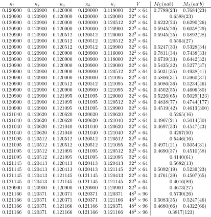
H and L masses), together with two mass degenerate quark data, when there is no mixing. Thus we now make a simultaneous fit to eq. (50) using the available data: the unitary data from [12] (the 323_{×64 lattice data forM}

N, MΛ, MΣ,MΞ

in Table XXII) together with some lighter quark mass data on a 483_{×96 lattice.}

Specifically we have used 23 valence quark masses on the 323_{×64 lattice with}

(κl, κs) = (0.12090,0.12090), four valence quark masses on each of the 323×64

lat-tice ensembles (0.12104,0.12062), (0.121095,0.120512) and (0.121145,0.120413) and a further four on the 483_{×96 lattice ensemble with (0.121166,0.120371). All}

the fit data used are given in Appendix D.

There are two LO ( ˜A) and four NLO ( ˜B) coefficients to determine. Thus we have a six parameter fit for the fit functions in eq. (50). It was found advantageous to preserve the identity of the Σ and Λ particles whenever possible, so for the mass degenerate PQ results, eqs. (57) and (58) were used. In Table 3 we give the

˜

A1 10.17(12)

˜

A2 1.849(124)

˜

B1 13.71(4.19)

˜

B2 -20.02(4.70)

˜

B3 -4.125(5.742)

˜

B4 -30.63(5.97)

Table 3: Fit results for LO and NLO expansion coefficients.

results of this fit with bootstrap errors. With our normalisation for the expansion coefficients all the numbers are_∼O(10), except ˜A2 which is rather smaller. The

(MINUIT) fit used gave χ2_{/dof∼38/60∼0.6 per degree of freedom.}

Two simple plots which illustrate the fit results are first the completely mass degenerate case (when as discussed previously in section 6.1 all outer baryon, Σ and Λ masses are the same), which may be illustrated by defining

Secondly we can consider the ‘symmetric’ difference case (between Σ and Λ) by setting

Dsym_{ΣΛ ≡} M˜

2

Σ(aab)−M˜Λ2(aa′b)−M˜Σ2(bba) + ˜MΛ2(bb′a)

4(δµb−δµa)

= A˜2+ ˜B2(δµa+δµb). (78)

(Again in these expressions and elsewhere a′_{, a}′′_{, . . . are mass degenerate but} distinct quarks.) At this order DΣΛsym is just a function of δµa+δµb; at higher

orders (see Appendix C, eq. (106)) there are terms _∝ δµa−δµb. Note that the

choice for D_ΣΛsym tends to suppress them (and indeed eliminates them at NLO); this was the reason for the choice of this ‘symmetric derivative’.

For the SΣΛ we have the results shown in Fig. 3. For SΣΛ, the fit is very

0.0 0.1 0.2

δµa

0 5 10

SΣΛ

S_ΣΛ

Figure 3: SΣΛ versusδµa(SΣΛis defined in eq. (77)), together with a fit also given in

eq. (77). Points used in the fit are denoted by filled circles (those outside the fit range are given by open circles).

good and as indicated this could be easily extended to larger quark masses. As mentioned before ˜A1 is the relevant coefficient for mass splittings on the outer

baryon ring.

In Fig. 4 we plot DΣΛsym against δµa+δµb. We see that the data is not linear

inδµa+δµb. (As explained before we would not expect the data in this plot to

lie on a unique curve due to the possible presence in the fit of terms proportional to δµa−δµb. However due to the choice of DΣΛsym deviations should be small.)

0.0 0.1 0.2

δµa+δµb

0.0 0.5 1.0 1.5 2.0 2.5 3.0

DΣΛ

sym

D_ΣΛsym

Figure 4: Dsym_ΣΛ versusδµa+δµb, (D_ΣΛsym is defined in eq. (78)), together with the fit

also given in eq. (78). The same notation as in Fig. 3.

Σ–Λ mass splitting, this necessitates the restricted fit region, as compared to Fig. 3. (It should however also be noted that the unitary quark masses have

|δma| ∼<0.01.)

The reason for this behaviour is due to spin–spin interaction between the quarks. It is known (e.g. [16]) that in quark models the mass splittings are partially due to the QCD spin-spin interaction between the quarks. From the Dirac equation we know that the magnetic moment of a fermion _∝ 1/ma, this

holds in QCD too, for the chromomagnetic moment, which might suggest a spin– spin interaction of the form_∝ 1/(mamb). This has also recently been proposed

in [17].

6.3

The physical point

By considering the equivalent pseudoscalar SU(3) flavour breaking mass expan-sion as for the baryon octet and matching to the pseudoscalar meson masses gives

δm∗

u,δm∗d,δm∗s. Again note that by considering the outer ring of the pseudoscalar

octet, provided that the average quark mass ¯m is held constant, the expansion coefficients can be determined from partially quenched 2 + 1 flavour simulations rather than 1 + 1 + 1 flavour expansions. This was discussed in [1] (and in partic-ular the subtraction of QED effects) and we just quote the result of the analysis here, as given in Table 4. To cover uncertainties in electromagnetic effects arising from violations of Dashen’s theorem, we assign a relative error _∼ 15% to the splitting δm∗

δm∗

u δm∗d δm∗s

-0.01140(3) -0.01067(3) 0.02207(4)

Table 4: Results for the bare quark mass in lattice units at the physical point, slightly updated from [1].

6.4

Comparison with ‘fan’ plots

We now compare the fit results with the mass values along the unitary line, i.e. which describe the evolution of the baryon masses along a path from the SU(3) symmetric point down to the physical point in the isospin degenerate limit, i.e.

mu =md≡ml. For this comparison we take the physical quark mass, in lattice

units, from Table 4 as

δm∗

l ≡(δm∗u+δmd∗)/2 = −0.01103(2). (79)

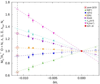
In Fig. 5 we show the ‘fan’ plot for all the ‘Σ’ and ‘Λ’ type particles. We have

N(lll′′_{)[= Λ}

3l(ll′l′′)], Λ(ll′s), Σ(lls), Ξ(ssl), Λ2sl(ss′l) and Ns(sss′′)[= Λ3s(ss′s′′].

(Ns(sss′′) and Λ2sl(ss′l) are fictitious baryons, but provide additional useful data

for the fits.) As this is the diagonal case there is no mixing and from eq. (38) the fit is given by ˜M2

N =PA1+PE+, ˜M

2

Λ =PA1−PE+. We find good agreement with the expected results.

It can easily be seen (‘ruler test’) that the fits are dominated by the LO in theSU(3) flavour symmetry breaking expansion. Given the fit results, this is not so surprising, as for the unitary results we have a maximum quark mass given by _|δml| ∼0.01, which is rather small (certainly in comparison with many of the

PQ masses used) and indicates that at least in the region we are interested in the low orderSU(3) flavour breaking expansion describes the data well.

For completeness we give here the values at the 2 + 1 QCD physical point (open circles in Fig. 5) of ˜M∗2

N = 0.6612(58), ˜MΛ∗2 = 0.9155(89), ˜MΣ∗2 = 1.052(4),

˜

M∗2

Ξ = 1.286(9), ˜MΛ∗22sl = 1.365(5) and ˜M

∗2

Ns = 1.687(6). For a comparison to these values, the stars in Fig. 5 represent the average of the squared experimental masses of the appropriate particles, as defined in the figure caption.

7

Results and Conclusions

We now give results for the QCD contribution to the baryon masses and their splittings.

7.1

Outer ring of the baryon octet

−0.010 −0.005 0.000 δm_l

0.6 0.8 1.0 1.2 1.4 1.6 1.8

MO

2 /X

N

2 O = N,

Λ

,

Σ

,

Ξ

,

Λ2sl

, N

s

pure QCD N(lll’’)

Λ(ll’s)

Σ(lls)

Ξ(ssl)

Λ2sl(ss’l)

Ns(sss’’)

sym. pt.

Figure 5: The baryon ‘fan’ plot for the ‘Σ’ and ‘Λ’ type particles ˜M2

O (O = N, Λ,

Σ, Ξ, Λ2sl,Ns) versus δml. Filled up triangles, squares, left triangles, right triangles,

diamonds and down triangles are the N(lll′′_{), Λ(ll}′_{s), Σ(lls), Ξ(ssl), Λ}

l2s(ss′l) and Ns(sss′′) results respectively using 323 ×64 sized lattices. The common symmetric

point is the filled circle. The open up triangles, left triangles, right triangles, down-triangles are from comparison 243 _×48 sized lattices (and not used in the fits here). The vertical dashed line from eq. (79) is thenf = 2 + 1 pure QCD physical point, with

the open circles being the numerically determined pure QCD hadron mass ratios for 2 + 1 quark flavours. For comparison, the stars represent the average of the (mass)2 of M∗2

N (lll′′) = (Mnexp 2(ddu) +Mpexp 2(uud))/2, MΛ∗2(lls) = MΛexp 20 (uds), M_Σ∗2(lls) = (M_Σexp 2− (dds) +M

exp 2

Σ+ (uus))/2 andM_Ξ∗2(ssl) = (M

exp 2

Ξ− (ssd) +M

exp 2

Ξ0 (ssu))/2.

in the ms – ml plane does not quite go through the physical point, while the

systematic errors arising from a finite lattice spacing are small.

We find the results for the masses and splittings of Table 5. For the splittings,

particle exp [GeV] result [GeV]

Mp uud 0.9383 0.9427(41)(40)

Mn ddu 0.9396 0.9454(40)(40)

MΣ+ uus 1.1894 1.1874(23)(50)

MΣ− dds 1.1974 1.1947(22)(51)

MΞ0 ssu 1.3149 1.3145(49)(56)

MΞ− ssd 1.3217 1.3191(48)(56)

splitting result [MeV]

Mn−Mp 2.70(15)(11)(40)

MΣ−−M_Σ+ 7.27(22)(31)(109)

MΞ−−M_Ξ0 4.57(19)(19)(68)

Table 5: Left panel: Baryon masses on the outer ring of the octet. The second column gives the quark content, while the third column, ‘exp’, gives the experimental masses from [2]. The last column, ‘result’, gives the result from this work. The first error is the statistical error, while the second is the total systematic error (in quadrature). X_Nexp

from eq. (48) has been used to convert to GeV. Right panel: Baryon mass splittings on the outer ring. The third error is due to possible violations in Dashen’s theorem, section 6.3.

rather than using eq. (50) directly (i.e. the results of the left panel of Table 5) we use the expressions in section 4.2. As discussed there, for the central values it makes little difference, however the error is now better determined. For the baryons on the outer ring of the octet the central values (both for masses and mass splittings) are in agreement with previous results, [1]. Note that we are not trying to compare the mass splittings with the experimental values, due to electromagnetic effects (not considered here).

7.2

Σ

–

Λ

mixing

We now turn to the result for Σ – Λ mixing. In Table 6 we give the Σ0 _{and Λ}0

particle exp [GeV] result [GeV]

MΣ0 uds 1.1926 1.1910(23)(51)

MΛ0 uds 1.1157 1.1109(54)(47)

Table 6: Σ0 and Λ0 masses. The same notation as for the left panel of Table 5.

masses. The Σ0 _{– Λ}0 _{mass difference is}

(The same discussion for the determination of the errors as for the previous results, section 7.1, also holds here.) This is to be compared with the experi-mental result, eq. (2) of 76.96(2) MeV. As both particles have the same quark content (and are uncharged) we do not expect much electromagnetic contribu-tion. Between the LO and NLO result there is only a few percent difference. Furthermore taking the difference between theMΣ0 −M_Λ0 mass splitting in Ta-ble 6 and M∗

Σ(lls)−MΛ∗(ll′s) (i.e. the isospin limit) gives a tiny contribution due

to isospin breaking, consistent with zero and which our present results are not precise enough to reliably estimate.

For the mixing angle we find

tan 2θΣΛ = 0.0123(45)(25), (81)

which, as anticipated, gives a very small angle, θΣΛ ∼ 0.006(3) rads<_∼1o.

Com-paring with e.g. a quark model result [7] givesθΣΛ ∼0.01 rads which is compatible

with our result.

We note that the LO value of tan 2θΣΛ from eq. (59) is∼0.0191 so in this case

with our determined ˜A and ˜B values for the SU(3) flavour breaking expansion, there is some reduction in the value of the angle when going to NLO. However in distinction to the Σ0 _{– Λ}0 _{mass difference the non-leading term is now much}

larger. This is because numerically (δms−δmu)(δms−δmd)/3δms|∗ ∼ 0.0166

to be compared with 3δmuδmdδms/2(δm2u +δm2d+δm2s)|∗ ∼ 0.0056, which as

expected from the discussion in section 4.2 is a factor 3 smaller. Thus theSU(3) symmetry flavour breaking expansion for the mixing angle in eq. (59) appears less convergent than for the Σ0 _{– Λ}0 _{mass difference, eq. (61). In order to account for}

this, we have increased the relative systematic error associated with the flavour symmetry expansion to _∼15%.

7.3

Conclusions

In this article we have extended our earlier work describing the QCD contribution to isospin breaking effects in baryon masses [1] to now also include states with the same quantum numbers, in this case the Σ0 _{and Λ}0_{, and their isospin mixing.}

This gives a complete description of theSU(3) flavour symmetry expansion of the (baryon) octet. As an example we have numerically investigated Σ0 _{– Λ}0 _mixing.

Acknowledgements

Appendix

A

Mass matrix symmetries – an example

To illustrate the transformations of the hadron mass matrices with an explicit example, let us write out in full the symmetry matrices for the transformation

u_↔d. A 3_×3 SU(3) matrix which exchanges the u and d quarks in the quark mass matrix eq. (8) is (see [12], eq. (128))

U = exp

iπ

2(λ1+

√

3λ8)

=



 

0 ₋1 0

−1 0 0

0 0 ₋1





 . (82)

(The minus signs ensure that _|U_| = 1, as required for an SU(3) matrix). If we act with this U on the quark mass matrix it simply swaps the u and d quark masses.

U



 

mu 0 0

0 md 0

0 0 ms   U †₌   

md 0 0

0 mu 0

0 0 ms 



 . (83)

To transform the baryon mass matrix we need an 8_×8 matrix corresponding to eq. (82).

U = exp

iπ

2(λ1 +

√

3λ8)

=               

0 1 0 0 0 0 0 0 1 0 0 0 0 0 0 0 0 0 0 0 0 1 0 0 0 0 0 ₋1 0 0 0 0 0 0 0 0 1 0 0 0 0 0 1 0 0 0 0 0 0 0 0 0 0 0 0 1 0 0 0 0 0 0 1 0

               . (84)

found by using an 8_×8 set of λ matrices (defined in [12], eq. (144)).

What happens to the baryon mass matrix when we rotate it with this U?

U                M2

n 0 0 0 0 0 0 0

0 M2

p 0 0 0 0 0 0

0 0 M2

Σ− 0 0 0 0 0

0 0 0 M2

ΣΣ MΣΛ2 0 0 0

0 0 0 M2

ΛΣ MΛΛ2 0 0 0

0 0 0 0 0 M2

Σ+ 0 0

0 0 0 0 0 0 M2

Ξ− 0

0 0 0 0 0 0 0 M2

Ξ0               

=



             

M2

p 0 0 0 0 0 0 0

0 M2

n 0 0 0 0 0 0

0 0 M2

Σ+ 0 0 0 0 0

0 0 0 M2

ΣΣ −MΣΛ2 0 0 0

0 0 0 ₋M2

ΛΣ MΛΛ2 0 0 0

0 0 0 0 0 M2

Σ− 0 0

0 0 0 0 0 0 M2

Ξ0 0

0 0 0 0 0 0 0 M2

Ξ− 

             

.

The n and p switch masses, as do the Σ− _{and Σ}+ _{and the Ξ}0 _{and Ξ}−_{, all as} expected whenu_↔d. In the central block, which tells us about the Σ0_Λ0 _sector,

we see that the diagonal entries are unchanged; the off-diagonal entries have their sign flipped. This is just what should happen underu_↔d; the eigenvalues (masses of the two states) will be the same, but the mixing angle will be reversed,

θΣΛ→ −θΣΛ.

B

The octet baryon mass matrix

B.1

The outer octet baryon masses

Here we discuss the mass matrix for partially quenched octet baryons in more detail than we could in the body of the paper. The arguments given here are similar to those given in section B.4 of [12] for the meson mass matrix, and in section 4.1 for the partially quenched decuplet mass formula.

If we have a diagonal quark mass matrix, strangeness, ‘upness’ and ‘downness’ are all conserved quantum numbers. There are therefore only ten non-zero entries in the 8_×8 octet mass matrix, namely the eight diagonal entries, and the two entries corresponding to Σ – Λ mixing. Σ – Λ mixing is permitted because both baryons have the same flavour content (uds); any other mixing would violate flavour conservation.

Since there are ten non-zero entries, we can express the mass matrix in terms of a basis of ten 8_×8 matrices. In [12] we classified these ten matrices according to their symmetries; see Table 1. Seven of the matrices are diagonal, they can be read off directly from the table. The table also contains three matrices which mix the Σ and Λ.

N1=           

1 0 0 0 0 0 0 0 0 1 0 0 0 0 0 0 0 0 1 0 0 0 0 0 0 0 0 1 0 0 0 0 0 0 0 0 1 0 0 0 0 0 0 0 0 1 0 0 0 0 0 0 0 0 1 0 0 0 0 0 0 0 0 1

          

N2=

          

−1 0 0 0 0 0 0 0 0 −1 0 0 0 0 0 0 0 0 0 0 0 0 0 0 0 0 0 0 0 0 0 0 0 0 0 0 0 0 0 0 0 0 0 0 0 0 0 0 0 0 0 0 0 0 1 0 0 0 0 0 0 0 0 1

          

N3=

          

−1 0 0 0 0 0 0 0 0 1 0 0 0 0 0 0 0 0 −2 0 0 0 0 0 0 0 0 0 0 0 0 0 0 0 0 0 0 0 0 0 0 0 0 0 0 2 0 0 0 0 0 0 0 0 −1 0 0 0 0 0 0 0 0 1

          

N4=

          

1 0 0 0 0 0 0 0 0 1 0 0 0 0 0 0 0 0 −2 0 0 0 0 0 0 0 0 −2 0 0 0 0 0 0 0 0 2 0 0 0 0 0 0 0 0 −2 0 0 0 0 0 0 0 0 1 0 0 0 0 0 0 0 0 1

          

N5=

           

−1 0 0 0 0 0 0 0 0 1 0 0 0 0 0 0 0 0 0 0 0 0 0 0 0 0 0 0 2

√

3 0 0 0

0 0 0 √2

3 0 0 0 0

0 0 0 0 0 0 0 0 0 0 0 0 0 0 1 0 0 0 0 0 0 0 0 −1

           

N6=

          

1 0 0 0 0 0 0 0 0 1 0 0 0 0 0 0 0 0 1 0 0 0 0 0 0 0 0 −3 0 0 0 0 0 0 0 0 −3 0 0 0 0 0 0 0 0 1 0 0 0 0 0 0 0 0 1 0 0 0 0 0 0 0 0 1

           (86)

N7=

          

1 0 0 0 0 0 0 0 0 1 0 0 0 0 0 0 0 0 −2 0 0 0 0 0 0 0 0 3 0 0 0 0 0 0 0 0 −3 0 0 0 0 0 0 0 0 −2 0 0 0 0 0 0 0 0 1 0 0 0 0 0 0 0 0 1

          

N8=

          

−1 0 0 0 0 0 0 0 0 1 0 0 0 0 0 0 0 0 0 0 0 0 0 0 0 0 0 0 −√3 0 0 0 0 0 0 −√3 0 0 0 0 0 0 0 0 0 0 0 0 0 0 0 0 0 0 1 0 0 0 0 0 0 0 0 −1

          

N9=

          

1 0 0 0 0 0 0 0 0 −1 0 0 0 0 0 0 0 0 −1 0 0 0 0 0 0 0 0 0 0 0 0 0 0 0 0 0 0 0 0 0 0 0 0 0 0 1 0 0 0 0 0 0 0 0 1 0 0 0 0 0 0 0 0 −1

          

N10=

          

0 0 0 0 0 0 0 0 0 0 0 0 0 0 0 0 0 0 0 0 0 0 0 0 0 0 0 0 −i 0 0 0 0 0 0 i 0 0 0 0 0 0 0 0 0 0 0 0 0 0 0 0 0 0 0 0 0 0 0 0 0 0 0 0

          

These matrices are orthogonal, in the sense Tr[NiNj] = 0 if i6=j.

We can write the (mass matrix)2 _{in terms of the basis matrices}

M2 ₌X i