This is a repository copy of Multiscale modelling and identification of a class of lattice dynamical systems.
White Rose Research Online URL for this paper: http://eprints.whiterose.ac.uk/74642/
Monograph:
Guo, L.Z., Billings, S.A. and Coca, D. (2009) Multiscale modelling and identification of a class of lattice dynamical systems. Research Report. ACSE Research Report no. 987 . Automatic Control and Systems Engineering, University of Sheffield
[email protected] https://eprints.whiterose.ac.uk/
Reuse
Unless indicated otherwise, fulltext items are protected by copyright with all rights reserved. The copyright exception in section 29 of the Copyright, Designs and Patents Act 1988 allows the making of a single copy solely for the purpose of non-commercial research or private study within the limits of fair dealing. The publisher or other rights-holder may allow further reproduction and re-use of this version - refer to the White Rose Research Online record for this item. Where records identify the publisher as the copyright holder, users can verify any specific terms of use on the publisher’s website.
Takedown
If you consider content in White Rose Research Online to be in breach of UK law, please notify us by
Multiscale modelling and identification of a
class of lattice dynamical systems
Guo, L. Z., Billings, S. A. and Coca, D.
Department of Automatic Control and Systems Engineering
University of Sheffield
Sheffield, S1 3JD
UK
Multiscale modelling and identification of a
class of lattice dynamical systems
Guo, L. Z., Billings, S. A., and Coca, D.
Department of Automatic Control and Systems Engineering
University of Sheffield
Sheffield S1 3JD, UK
Abstract
A new multiscale modelling framework is introduced to describe a class of lattice dy-namical systems (LDS), which can be used to model natural systems involving multiphysics and the multi-resolution facets of a single spatio-temporal dynamical system. The emphasis of the paper is on the multi-resolution facets, with respect to the spatial domain, of a single spatio-temporal dynamical system by using a Haar wavelet decomposition technique. A multiscale identification method for such systems is then proposed, which can be consid-ered as a dual of the multigrid method. The proposed identification method involves three steps: the system dynamics at some specific scale of interest are identified using a recur-sive least-squares algorithm; the residual is then projected onto coarser scales using Haar wavelets and the parameter estimation errors are minimized; and finally a coarse correction procedure is applied to the original scale. An outstanding advantage of the proposed iden-tification method is a saving on the computational costs. Numerical examples are provided to demonstrate the application of the proposed new approach.
1
Introduction
Lattice dynamical systems (LDS) and the subset coupled map lattices (CML), are systems of
differential equations, indexed by points in a homogeneous lattice such as the d-dimensional
integer lattice Zd, which incorporates some aspect of the spatial structure of the lattice. These
hierarchical structure on homogeneous lattices (Hilgers and Beck 1999). All these studies have significantly enriched the theory and applications of lattice dynamical systems and motivated an investigation of such systems from a multiscale point of view which is described in this paper.
As a generalisation to the above models, a multiscale modelling framework is introduced in this paper to describe a class of lattice dynamical systems, which can be used to model both sys-tems involving multiphysics in nature and the multi-resolution facets of a single spatio-temporal dynamical system. Actually multiscale methods have been extensively studied for the past two decades with applications in the field of applied sciences (Glimm and Sharp 1997, Krumhansl 2000, and Li and Kwauk 2003). This has been mainly driven by the requirements of the analysis of the systems which involve natural multiscale effects such as molecular dynamics and by the progress of computational capability both in software and hardware. Apart from these multiscale methods, it is also interesting to investigate a single spatio-temporal dynamical system from a multiscale or multi-resolution point of view. There are some advantages of doing this for a sin-gle dynamical system: i) it may reduce the computational cost if a coarser scale can be used; ii) it can separate high frequency components from low frequency components so as to be able to deal with these separately. Some multiscale modelling methods are described in the litera-ture, including a multiscale theory for linear dynamic processes (Stephanopoulos, Karsligil, and Dyer 2008), the heterogeneous multiscale method (E, Engquist, Li, Ren, and Vanden-Eijnden 2007), the multiscale modelling of cancer (Martins, Ferreira Jr., and Vilela 2007), the variational multiscale method (Hughes, Frijoo, Mazzwi, and Quincy 1998), Bayesian multiscale modelling (Ferreira and Lee 2007), and multiscale autoregressive models (Daoudi, Frakt, and Willsky 1999). All of these methods made important contributions to multiscale theory and applications from different individual perspectives. The emphasis of the current paper is on the multi-resolution facets, with respect to the spatial domain, of a single spatio-temporal dynamical system and on multiscale parameter estimation using a Haar wavelet decomposition technique. The multiscale identification method for such systems can be considered as a dual of the multigrid method. The proposed identification method involves three steps: the system dynamics at some specific scale of interest are identified using a recursive least-squares algorithm; the residual is then projected onto coarser scales using Haar wavelets and the parameter estimation errors are minimized; and finally a coarse correction procedure is applied to the original scale. An outstanding advantage of the proposed identification method is a saving of the computational costs.
2
Multiscale lattice dynamical systems
2.1
Lattice dynamical systems (LDS)
In this section, lattice dynamical systems are introduced and definitions and terminology used
later are summarised. Let Λ∈Zdbe and-dimensional integral periodic lattice of points. Lattice
dynamical systems defined over the d−dimensional integral lattice Λ can be described by the
following system
u(t) =F(u(t−1)), t= 1,2,· · · (1) for the discrete-time case, or
˙
u(t) =F(u(t)), t≥0 (2)
for a continuous-time description, in which u = {ui}i∈Λ ∈ H (i will be a multi-indexed array
when d > 1) is the state of the system and t represents the time instant. H, the phase space
of the system, can be the Banach space or Hilbert space l∞
= {u : u∞ = supi∈Λ|ui| < +∞}
or l2 ={u :u
2 = (i∈Λ|ui|2)1/2 <+∞} and F is an operator over H. Equation (2) actually
represents an infinite system of (coupled) differential equations, one equation at each point of the lattice representing the local dynamics at that specific point interacting with other lattice points. In this paper we consider the case of systems with finite-range interaction, and which are
invariant under translations of the lattice. Let a finite subsetQ∈Λ of lattice points be the fixed
neighbours which will describe the range of the coupling. In this case, equation (2) can be given
more specifically at each lattice point, by defining a map F :H →H,F(u)i =F({ui+i′}i′∈Q), as
follows
u(i, t) =u(t)i =F(u(t−1))i =F({u(i+i′, t−1)}i′∈Q), t= 1,2,· · ·, i∈Λ (3)
for discrete-time case, or
˙
u(i, t) = ˙u(t)i =F(u(t))i =F({u(i+i′, t)}i′∈Q), t≥0, i∈Λ (4)
for continuous-time case, where the mapF can be in C1, Cp, or C∞
depending on the problems concerned. Various properties of solutions for lattice dynamical systems can be found in the literature under a variety of assumptions on the structure and parameters of the systems including linear and nonlinear cases.
2.2
Multiscale lattice dynamical systems (MLDS)
the spatio-temporal dynamical evolution at each site within a multiscale environment: a term describing the reaction behaviour, a term describing the coupling with other lattice points within the same spatial scale, and a term describing the coupling between different scales.
Similar to the previous discussion, the d-dimensional integral lattice Zd is considered as the
basic spatial structure. A multiscale lattice dynamical system with M scales is defined here as a
d-dimensional lattice Zd where each site evolves at scale m, m= 0,1,· · ·, M in time through a
map of the form:
um(i, t) =Rm(um(i, t−1)) +D1m({um(i+i′
, t−1)}i′∈Q) +Dm2 ({um
′
(i+i′
, t−1)}i′∈Q′,m′∈S′) (5)
m= 0,1,· · ·, M, m′
=m∈S′
⊂ {0,1,2,· · ·, M}, t= 1,2,· · ·, for the discrete-time case, and
˙
um(i, t) =Rm(um(i, t)) +D1m({um(i+i′
, t)}i′∈Q) +Dm2 ({um
′
(i+i′
, t)}i′∈Q′,m′∈S′) (6)
m = 0,1,· · ·, M, m′
= m ∈ S′
⊂ {0,1,2,· · ·, M}, for the continuous-time case, where um(i, t)
denotes the field value at site i, at the indicated time t, and at scale m. The three terms in
the right hand side of eqn. (6) determine the dynamics of the system: (a) the first term Rm(·)
accounts for the local reaction at its own spatial level m, (b) the second term Dm
1 (·) represents
the diffusive coupling within the same spatial level m with neighbour Q, and (c) the last term
Dm
2 (·) indicates the diffusive coupling between different spatial scales, where S
′
denotes the levels involved. The multiscale lattice dynamical system model (6) describes a large class of spatio-temporal dynamical systems. The following are two important examples in the literature regarding multiscale modelling of spatio-temporal systems.
• Hierarchical CML (Hilgers and Bech 1999). Hierarchical CML was proposed to model
hydrodynamical turbulence by Higers and Bech. They used these lattice dynamical systems to improve the efficiency of the simulation of the spatio-temporal stochastic processes. Interestingly, the hierarchical structure proposed by them is not towards the lattice itself but rather the levels of the energy cascade. The hierarchical CML can be treated as a special class of the proposed multiscale lattice dynamical systems, where
R(um(i, t)) = λmum(i, t)
D1m(um(i, t)) =
nearest neighboursσ
um(i+σ, t)
D2m(um(i, t)) = ξm(t)um−1
(i, t) (7)
• Coupled maps on hierarchical lattices (Cosenza and Tucci, 2000). These models were
Fm(um(i, t)) = (1−kγ)um(i, t)
Dm1 (um(i, t)) = 0
Dm2 (um(i, t)) = γ
daughters d
um+1(id, t) +γ
parents p
um−1(i
p, t) (8)
2.3
Haar wavelet multiresolution as multiscale lattice dynamical
sys-tems
In this section, we will consider how to obtain a multiscale LDS model from a linear LDS model through a Haar wavelet multiresolution analysis. As a special class of multiscale lattice dynamical systems, the multiscale models obtained in this way are essentially multiresolution facets, with respect to the spatial domain, of a single lattice dynamical system model. The Haar wavelets and multiresolution analysis theory can be found in Chui (1992). For the purpose of clarity and simplicity and without loss of generalisation, a one-dimensional linear lattice dynamical system with the two nearest neighbours is considered as an example system in this paper
u(i, t) =a0u(i, t−1) +a1u(i+ 1, t−1) +a−1u(i−1, t−1) +b0f(i, t−1), t= 1,2,· · ·, i∈Z (9)
where the coefficients a0, a1, and a−1 can be interpreted as associated with the reaction and the
coupling parameters, and b0 is the control parameter for the external input f.
2.3.1 Multi-resolution representation
From a multiscale point of view, the LDS (9) can be considered as an approximation of an
underlying spatio-temporal system in a space V2m, which we will consider as at its finest scale
available. It follows that (9) can be rewritten explicitly as
um
a(i, t) =a0uma(i, t−1) +a1uma(i+ 1, t−1) +a−1uma(i−1, t−1) +b0fam(i, t−1), t= 1,2,· · ·, i∈Z
(10)
Let um
a(k, t) and umd(k, t) be the Haar wavelet approximation and detail coefficients at the mth
scale and kth shift with respect to spatial variable i, and at time instant t. Then the wavelet
decomposition and reconstruction formula between scales m and m−1 for the signalu(i, t) are
um−1
a (k, t) =
1
√
2u
m
a(2k, t) +
1
√
2u
m
a(2k+ 1, t)
um−1
d (k, t) =
1
√
2u
m
a(2k, t)−
1
√
2u
m
and
um
a(2k, t) =
1
√
2u
m−1
a (k, t) +
1
√
2u
m−1
d (k, t)
uma(2k+ 1, t) = √1
2u
m−1
a (k, t)−
1
√
2u
m−1
d (k, t) (12)
Note that the above approximation equation can be equivalently written as the following two
equations fork an even number
um−1
a (
k
2, t) =
1
√
2u
m
a(k, t) +
1
√
2u
m
a(k+ 1, t)
um−1
a (
k
2 + 1, t) =
1
√
2u
m
a(k+ 2, t) +
1
√
2u
m
a(k+ 3, t) (13)
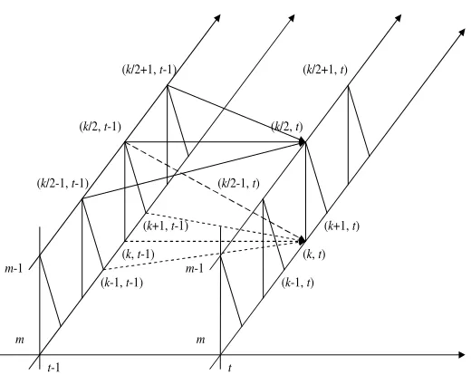
This relationship is shown in the tree in Fig.1.
From eqns. (13) and (10), many different multiscale relationships including coarse-to-fine, fine-to-coarse, and the lattice dynamical systems at different scales can be derived depending on the applications. Some of these will be derived and shown in the next two sections.
2.3.2 Lattice dynamical systems without external inputs
Given a linear lattice dynamical system (9) and its fine-scale approximation (10) withf = 0, the
following multiscale dynamical relations can be obtained
a). Coarse-to-fine equations (assume that k is an even number)
uma(k, t) = (a0−a1)uma(k, t−1) +a−1uma(k−1, t−1) +
√
2a1uma−1(
k
2, t−1)
uma(k+ 1, t) = (a0−a−1)uam(k+ 1, t−1) +a1uma(k+ 2, t−1) +
√
2a−1uma−1(
k
2, t−1)(14)
b). Fine-to-coarse equations (assume thatk is an even number)
um−1
a (
k
2, t) = a0u
m−1
a (
k
2, t−1) +
√
2
2 (a1u
m
a(k+ 2, t−1) +a1uma(k+ 1, t−1)
+a−1uma(k, t−1) +a−1uma(k−1, t−1))
um−1
a (
k
2 + 1, t) = a0u
m−1
a (
k
2 + 1, t−1) +
√
2
2 (a1u
m
a(k+ 4, t−1) +a1uma(k+ 3, t−1)
t-1 t m-1
m
m-1
m
(k,t) (k+1,t)
(k-1,t) (k,t-1)
(k+1,t-1)
(k-1,t-1)
(k/2,t) (k/2+1,t)
(k/2-1,t) (k/2-1,t-1)
[image:9.612.138.398.242.449.2](k/2,t-1) (k/2+1,t-1)
c). Lattice dynamical system equations at scale m−1
um−1
a (
k
2, t) = 2a0u
m−1
a (
k
2, t−1) + (−
a2 0
2 + 2a1a−1)u
m−1
a (
k
2, t−2) +a
2 −1um
−1
a (
k
2 −1, t−2)
+a21um−1
a (
k
2 + 1, t−2) (16)
The coarse and fine relationships (14) in a) and (15) in b) can be easily derived as follows.
Because of the nature of the tree structure by Haar wavelets, that is, (k/2, t) is the average of
(k, t) and (k+ 1, t) while (k/2 + 1, t) is the average of (k+ 2, t) and (k+ 3, t)(see Fig. 1), there
is a need to distinguish the case where k is an even number or an odd number when considering
the lattice dynamics (10) at (k, t) and (k+ 1, t). Rewritting (10) for k and k+ 1 (k is assumed
to be even) as follows
uma(k, t) = a0uma(k, t−1) +a1uam(k+ 1, t−1) +a−1uma(k−1, t−1)
uma(k+ 1, t) = a0uma(k+ 1, t−1) +a1uma(k+ 2, t−1) +a−1u
m
a(k, t−1) (17)
Inserting (13) yields (14) while adding the two equations in (17) together and using (13) again yields (15).
The relationship (16) at scalem−1 in c) can be done by introducing a spatial translation operator
Sp :Spu(k, t) =u(k+p, t) and a temporal translation operatorTq :Tqu(k, t) = u(k, t+q). Then
it follows that they have the following simple properties
• S0u(k, t) =u(k, t) and T0u(k, t) =u(k, t);
• Sp1Sp2 =Sp1+p2,Tq1Tq2 =Tq1+q2, p
1, p2, q1, q2 ∈R;
• SpTq=TqSp with TqSpu(k, t) =u(k+p, t+q),p, q∈R;
• Spau(k, t) =au(k+p, t) and Tqau(k, t) = au(k, t+q),p, q∈R, a∈R.
To derive the lattice dynamical model at scalem−1 from scalem, will require the reconstruction
equations. Rewritting the reconstruction equations (12) for k even as follows
uma(k, t) = √1
2u
m−1
a (
k
2, t) +
1
√
2u
m−1
d (
k
2, t)
uma(k+ 1, t) = √1
2u
m−1
a (
k
2, t)−
1
√
2u
m−1
d (
k
2, t)
uma(k+ 2, t) = √1
2u
m−1
a (
k
2+ 1, t) +
1
√
2u
m−1
d (
k
2 + 1, t)
uma(k+ 3, t) = √1
2u
m−1
a (
k
2+ 1, t)−
1
√
2u
m−1
d (
k
Substituting um
a(k, t), uma(k+ 1, t−1), uma(k−1, t−1) given directly or indirectly by (18) into
(10) with k an even number yields
1
√
2u
m−1
a (
k
2, t) +
1
√
2u
m−1
d (
k
2, t) = a0(
1
√
2u
m−1
a (
k
2, t−1) +
1
√
2u
m−1
d (
k
2, t−1)))
+a1(
1
√
2u
m−1
a (
k
2, t−1)−
1
√
2u
m−1
d (
k
2, t−1)))
+a−1(
1
√
2u
m−1
a (
k
2 −1, t−1)−
1
√
2u
m−1
d (
k
2 −1, t−1)))
(19)
Rearranging gives
(um−1
a (
k
2, t)−(a0 +a1)u
m−1
a (
k
2, t−1)−a−1u
m−1
a (
k
2 −1, t−1))
+(um−1
d (
k
2, t)−(a0−a1)u
m−1
d (
k
2, t−1) +a−1u
m−1
d (
k
2 −1, t−1)) = 0 (20)
and with the spatial and temporal operators
(1−(a0+a1)T−1−a−1T−1S−1)uma−1(
k
2, t) + (1−(a0−a1)T
−1+a
−1T−1S−1)umd−1(
k
2, t) = 0 (21)
By repeating the same procedure, the following equation for the case of k+ 1 can be given
(1−(a0+a−1)T−1−a1T−1S1)uma−1(
k
2, t) + (−1 + (a0−a−1)T
−1
−a1T−1S1)umd−1(
k
2, t) = 0 (22)
By solving the equations (21) and (22) through eliminating the details ud, yields
(−2 + 4a0T−1+ (−a20+ 4a1a−1)T−2+ 2a2−1T
−2S−1+ 2a2 1T
−2S1)um−1
a (
k
2, t) = 0 (23)
which gives the lattice dynamical model at scale m− 1 (16) by expressing the system in its
conventional way without the operators.
2.3.3 Lattice dynamical systems with external inputs
For the linear lattice dynamical systems with external inputf, the following multiscale dynamical
a). Coarse-to-fine equations (assume that k is an even number)
uma(k, t) = (a0−a1)uma(k, t−1) +a−1u
m
a(k−1, t−1) + √
2a1uma−1(
k
2, t−1)
+b0fam(k, t−1)
uma(k+ 1, t) = (a0−a−1)uam(k+ 1, t−1) +a1uma(k+ 2, t−1) +
√
2a−1uma−1(
k
2, t−1)
+b0fam(k+ 1, t−1) (24)
b). Fine-to-coarse equations (assume thatk is an even number)
um−1
a (
k
2, t) = a0u
m−1
a (
k
2, t−1) +
√
2
2 (a1u
m
a(k+ 2, t−1) +a1uma(k+ 1, t−1)
+a−1uma(k, t−1) +a−1uam(k−1, t−1)) +b0fam(k, t−1)
um−1
a (
k
2 + 1, t) = a0u
m−1
a (
k
2 + 1, t−1) +
√
2
2 (a1u
m
a(k+ 4, t−1) +a1uma(k+ 3, t−1)
+a−1uma(k+ 2, t−1) +a−1uam(k+ 1, t−1)) +b0fam(k+ 1, t−1) (25)
c). Lattice dynamical system equations at scale m−1
um−1
a (
k
2, t) = 2a0u
m−1
a (
k
2, t−1) + (−
a2 0
2 + 2a1a−1)u
m−1
a (
k
2, t−2) +a
2 −1um
−1
a (
k
2−1, t−2)
+a21um−1
a (
k
2 + 1, t−2) +b0f
m−1
a (
k
2, t−1)−
1
2(2a0−a−1−a−1)b0f
m−1
a (
k
2, t−2)
+a1b0
2 f
m−1
a (
k
2 + 1, t−2) +
a−1b0
2 f
m−1
a (
k
2 −1, t−2)−
1
2(a1−a−1)b0f
m−1
a (
k
2, t−2)
+a1b0
2 f
m−1
a (
k
2 + 1, t−2)−
a2b0
2 f
m−1
a (
k
2−1, t−2) (26)
The coarse and fine relationships (14) in a) and (15) in b) can be obtained in the similar way as
above. The relationship (16) at scale m−1 in c) can be treated in a similar way but with an
extra term representing the forces, where the equations to be solved are
(1−(a0+a1)T−1 − a−1T−1S−1)uma−1(
k
2, t) + (1−(a0 −a1)T
−1+a
−1T−1S−1)umd−1(
k
2, t)
= b0T−1(fam−1(
k
2, t) +f
m−1
d (
k
2, t))
(1−(a0+a−1)T−1 − a1T−1S1)uma−1(
k
2, t) + (−1 + (a0 −a−1)T
−1
−a1T−1S1)umd−1(
k
2, t)
= b0T−1(fam−1(
k
2, t)−f
m−1
d (
k
3
Multiscale identification of the linear lattice dynamical
model
In this section, a least squares based multiscale method is proposed for the identification of the linear lattice dynamical system (10), that is
u(i, t) = a0u(i, t−1) +a1u(i+ 1, t−1) +a−1u(i−1, t−1), t= 1,2,· · ·, i∈Z (28)
3.1
Recursive least squares estimates of the parameters at scale
m
The approximation in finite dimensional space V2m can be written as
uma(i, t) =a0uma(i, t−1) +a1uma(i+ 1, t−1) +a−1uma(i−1, t−1) +wm(i, t) (29)
where t= 1,2,· · · and i= 0,1,· · ·,2m−1 or in matrix form as
ym(t) = φm(t−1)Tθm+wm(t) (30)
where ym(t) = (uma(0, t), uma(1, t),· · ·, uam(2m − 1, t))T, θm = (a−1, a0, a1)T, and the modelling
error vector or noise wm(t) = (wm(0, t), wm(1, t),· · ·, wm(2m−1, t))T, and
φm(t−1)T =
⎛
⎜ ⎜ ⎜ ⎜ ⎝
um
a(−1, t−1) uma(0, t−1) uma(1, t−1)
um
a(0, t−1) uma(1, t−1) uma(2, t−1)
...
um
a(2m−2, t−1) uma(2m−1, t−1) uma(2m, t−1)
⎞
⎟ ⎟ ⎟ ⎟ ⎠
(31)
in which the um
a(−1, t−1) and uma(2m, t−1) are the boundary conditions. A standard least
squares estimate to the problem (30) is given by
ˆ
θnm = (Rnm)−1n
t=1
φm(t−1)ym(t) (32)
with the least squares criterion
Jmn(θ) = 1 2
n
t=1
ym(t)−φm(t−1)Tθ2 (33)
where Rn
m =
n
t=1φm(t −1)φm(t− 1)T and n the number of time samplings. The recursive
estimation equation is
ˆ
θmn = ˆθn−1
m + (Rnm)
−1φ
For the deterministic case where wm(t) = 0 for allt, it follows that
Rnmθ˜nm =Rn−1
m θ˜n
−1
m =constant (35)
with ˜θn
m =θ
∗
m−θˆnm. It follows that limn→∞θ˜mn = 0 if limn→∞λminRnm =∞where λminRnm is the
smallest eigenvalue of Rn
m . In the stochastic case, it has been shown that if the noise wm(t) is
a martingale difference sequence, then under certain assumptions (e.g. Lai and Wei 1982) the
least squares estimate ˆθn
m of the true parameter θ
∗
m satisfies
θˆnm−θ∗
m2 =O(
logλmaxRnm
λminRnm
) (36)
provided thatλminRnm → ∞ as n→ ∞. Here λmaxRnm and λminRnm are the largest and smallest
eigenvalues of the matrix Rn
m. Moreover, the least squares estimates are strongly consistent if
λminRnm → ∞and the following excitation condition
lim
n→∞
logλmaxRnm
λminRnm →
0, a.s. (37)
is satisfied.
3.2
Multiscale view of the parameter estimation
In this section a coarser scale correction method to the least squares estimates obtained at certain
scale m will be presented. The proposed method is similar to the coarse grid correction to the
multigrid method but here this procedure is used in the parameter estimation process.
From the earlier discussion, the least squares estimates ˆθn
m of the system parameters θ
∗
m at scale
m leads to two possible errors: the first is the parameter estimate error ˜θn
m and the other is the
residual em(t) =ym(t)−φm(t−1)Tθˆnm. From (30), it follows that
em(t) = ym(t)−φm(t−1)Tθˆnm =φm(t−1)Tθm∗ +wm(t)−φm(t−1)Tθˆnm =φm(t−1)Tθ˜nm+wm(t) (38)
which shows the relationship between the residual and estimate errors of the least squares method. Consider the following criterion
Jm−1
m (ηm−1) =
1
2 < φm(t−1)
T(ˆθn
m+ηm−1),θˆmn +ηm−1 >−< ym(t),θˆnm+ηm−1 > (39)
where <·,·> denotes the bilinear form defined by
< u, v >=
2m
i=1
uivi, u, v ∈R2
m
A direct solution to the minimisation of (39) can be obtained easily as
φm(t−1)Tηm−1 =ym(t)−φm(t−1)Tθˆnm =em(t) (41)
which is in exactly the same form as the residual equation (38), which can be rewritten as
em(k, t) = ˜a0uma(k, t−1) + ˜a1uma(k+ 1, t−1) + ˜a−1u
m
a(k−1, t−1), i= 0,1,· · ·,2m−1 (42)
Projecting this equation from space V2m onto the coarser space V2m−1 by multiplying by the
2m−1
×2m Haar wavelet transform matrixP
P = √1
2 ⎛ ⎜ ⎜ ⎜ ⎜ ⎝
1 1 0 0 · · · 0 0
0 0 1 1 · · · 0 0
. ..
0 0 0 0 · · · 1 1
⎞ ⎟ ⎟ ⎟ ⎟ ⎠ (43)
on both sides of the eqn. (41) yields the following coarse relationship in coarse space V2m−1
φm−1(t−1)Tηm−1 =em−1(t) (44)
where em−1(t) = P em(t) = (em
−1
a (0, t), ema−1(1, t),· · ·, ema−1(2m−1−1, t))T, ηm−1 = (˜a−1,˜a0,˜a1)T,
and
φm−1(t−1)
T =P φ
m(t−1)T =
⎛ ⎜ ⎜ ⎜ ⎜ ⎝
um−1
a (0, t−1) um
−1
a (0, t−1) um
−1
a (1, t−1)
um−1
a (1, t−1) uma−1(1, t−1) uma−1(2, t−1)
.. . um−1
a (2m
−1−1, t−1) um−1
a (2m
−1−1, t−1) um−1
a (2m
−1, t−1)
⎞ ⎟ ⎟ ⎟ ⎟ ⎠ (45)
in which um−1
a (k+ 1, t−1) = 1/
√
2(um
a(2k+ 1, t−1) +uma(2k+ 2, t−1)), k= 0,1,· · ·,2m
−1−1.
Similar results can be achieved by using Haar wavelet detail transform Q
Q= √1
2 ⎛ ⎜ ⎜ ⎜ ⎜ ⎝
1 −1 0 0 · · · 0 0 0 0 1 −1 · · · 0 0
. ..
0 0 0 0 · · · 1 −1 ⎞ ⎟ ⎟ ⎟ ⎟ ⎠ (46)
Next let us see how the Haar wavelet transforms P and Q change the eigenvaules of the matrix
φm(t−1)φm(t−1)T. Firstly, notice that PTP +QTQ=I so that
φm(t−1)φm(t−1)T = φm(t−1)(PTP +QTQ)φm(t−1)T
By adding up both side of (47), it follows that
Rnm =Rnm−1+Hmn−1 (48)
whereHn
m−1 =
n
t=1φm(t−1)QTQφm(t−1)T. It is interesting to see that the covariance matrix
Rn
m at scale m can be divided into a low frequency part Rmn−1 and a high frequency part Hmn−1
at scale m−1. It can be checked that the 3×3 matrices φm(t−1)PTP φm(t−1)T and φm(t−
1)QTQφ
m(t−1)T have the same eigenvalues: 1/2(λ1(t−1)2+λ2(t−1)2),1/2λ3(t−1)2 assuming
that λ1(t−1)2, λ2(t−1)2, λ3(t−1)2 are the three eigenvalues of the matrixφm(t−1)φm(t−1)T.
This shows that the matrices φm(t−1)PTP φm(t−1)T and φm(t−1)QTQφm(t−1)T are only
semi-positive definite but this does not affect the positive definiteness of the matrixRl
m−1because
Rl
m−1 =
l
t=1φm(t−1)PTP φm(t−1)T =tl=1φm−1(t−1)φm−1(t−1)T will be positive definite
as long as φm−1(0)φm−1(0)T is chosen to be positive definite.
3.3
Convergence analysis
The proposed multiscale method involves the following three steps
• Recursive least squares estimates for the parameters at scale m;
• Recursive least squares estimates of the estimation errors of the parameters at scale m−1
• Coarse correction from m−1 to m
The coarse correction is accomplished by simply adding the coarse estimates to the fine estimates as follows
ˆ
θnm ←θˆmn + ˆηml −1 (49)
Applying the standard least squares method to the problem (44) again gives the following esti-mate
ˆ ηl
m−1 = (R
l m−1)
−1l
t=1
φm−1(t−1)em−1(t) (50)
where the matrix Rl
m−1 =
l
t=1φm−1(t−1)φm−1(t−1)T and l the number of time samplings.
For the deterministic case, again the least squares solution to (44) satisfies
Rlm−1η˜lm−1 =Rl −1
m−1η˜l −1
m−1 =constant (51)
with ˜ηl
m−1 =η ∗
m−1−ηˆml −1 = ˜θnm−ηˆlm−1. Now let ˜θnm+l =θ
∗
Rml −1θ˜
n+l
m = Rlm−1(θ ∗
m−(ˆθnm+ ˆηml −1)) (52)
= Rlm−1(θ
∗
m−θˆnm)−Rlm−1ηˆ
l m−1
= Rlm−1θ˜nm−Rlm−1ηˆml −1
= Rlm−1η˜ml −1
= Rl−1
m−1η˜l −1
m−1
= Rl−1
m−1θ˜n+(l −1)
m
so that
Rlm−1θ˜mn+l =Rl
−1
m−1θ˜n+(l −1)
m =constant (53)
Hence, since (Rl
m−1)+ is a sequence of decreasing semi-positive definite matrices, both (Rlm−1)+
and ˜θn+l
m converge. This shows that liml→∞θ˜nm+l= 0 if λminRml −1 → ∞. Moreover
(˜θnm+l)TRlm−1θ˜mn+l ≤(˜θn+(l
−1)
m )TRlm−1θ˜n+(l −1)
m ≤ · · · ≤(˜θnm)TR0m−1θ˜mn (54)
Since Rl
m−1 =R
l−1
m−1 +φm−1(l−1)φm−1(l−1)T, it has
λminRlm−1 ≥λminRml−−11 ≥ · · · ≥λminR0m−1 (55)
It follows that
θ˜nm+l2 ≤κ(Rl−1
m−1)θ˜n+l −1
m 2 (56)
and
θ˜mn+l2 ≤κ(R0m−1)θ˜mn2 (57)
where κ(R) =λmaxR/λminR is the condition number of the matrix R.
This shows that liml→∞θ˜nm+l = 0 if liml→∞λminRml −1 = ∞ when the system is deterministic,
where λminRlm−1 is the smallest eigenvalue of R
l m−1.
4
Numerical results
In this section, a numerical simulation is conducted to illustrate the proposed multiscale param-eter estimation method. We will continue to use the example system (10), that is
5 10 15 20 25 30 35 40 45 50 −0.1
0 0.1 0.2 0.3 0.4 0.5 0.6 0.7 0.8 0.9
Simulation steps
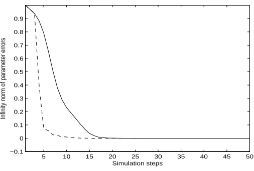
[image:18.612.185.438.80.251.2]Infinity norm of parameter errors
Figure 2: The parameter estimate errors for case 1 without noise (solid: LS at scale m, dashed:
Multiscale method)
where i = 0,1,· · ·,2m −1 representing an approximation in finite dimensional space V
2m. The
numerical studies are carried out for four different cases, chosen to illustrate the properties of the new algorithm.
Case 1. In this simulation, the parameters were chosen as a0 = 0.1, a1 = 0.5, a−1 = −0.2 and
m= 6. The initial conditions of the lattice dynamical system were
u(i,0) = sin(2iπ
2m) +
1
2sin(
16iπ
2m ) +
1
2sin(
32iπ
2m ) (59)
and Dirichlet boundary conditions were considered. The reason for the choice of this initial condition is to include different frequency components. The recursive least squares algorithm
was run for three simulation steps at fine scale m = 6 and then projected to coarse scale m= 5
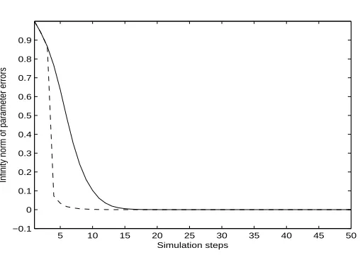
for the rest of the computation. Moreover, to test the performance of the proposed multiscale identification method, the same procedure was applied to the system with a white noise of zero
mean and std = 0.3. Fig.2 and Fig.3 shows the infinity norm of the parameter estimate errors
e(t)∞ for the cases without noise and with noise. These results indicate that the multiscale
identification method has a faster convergence rate than the conventional recursive least squares method.
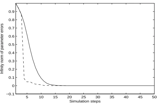
Case 2. In this case, the parameters were still chosen asa0 = 0.1, a1 = 0.5, a−1 =−0.2 andm= 6
but the initial conditions of the lattice dynamical system were chosen as a Gaussian white noise with zero mean and std = 1. The same procedure as in case 1 was employed and the results are shown in Fig.4 and Fig.5.
From all these numerical results, it can be observed that
5 10 15 20 25 30 35 40 45 50 −0.1
0 0.1 0.2 0.3 0.4 0.5 0.6 0.7 0.8 0.9
Simulation steps
[image:19.612.185.439.116.286.2]Infinity norm of parameter errors
Figure 3: The parameter estimate errors for case 1 with noise (solid: LS at scale m, dashed:
Multiscale method)
5 10 15 20 25 30 35 40 45 50
−0.1 0 0.1 0.2 0.3 0.4 0.5 0.6 0.7 0.8 0.9
Simulation steps
Infinity norm of parameter errors
Figure 4: The parameter estimate errors for case 2 without noise (solid: LS at scale m, dashed:
[image:19.612.186.440.437.617.2]5 10 15 20 25 30 35 40 45 50 −0.1
0 0.1 0.2 0.3 0.4 0.5 0.6 0.7 0.8 0.9
Simulation steps
[image:20.612.185.438.80.251.2]Infinity norm of parameter errors
Figure 5: The parameter estimate errors for case 2 with noise (solid: LS at scale m, dashed:
Multiscale method)
compared to applying the least squares method at a single scale.
2) Due to the projection from fine to coarse, the computational costs are reduced because of the reduction of the dimension of the problem.
5
Conclusions
A multiscale modelling framework for a class of lattice dynamical systems has been introduced. It has been demonstrated that the proposed framework not only includes many existing models as special cases but also connects the multiresolution analysis to the multiscale problem. Apart from that, a new multiscale identification method has been presented by using a Haar wavelet decomposition method and a recursive least squares algorithm. It has been shown by numerical studies that the convergence properties of the parameter estimation can be improved by the proposed multiscale method.
With the proposed framework, there are plenty of problems to be solved such as a detailed analysis of the convergence and consistency in the presence of noise and how to extend the proposed identification method to nonlinear lattice dynamical systems.
6
Acknowledgement
References
[1] Chow, S. and Mallet-Paret, J., (1995) Pattern Formation and Spatial Chaos in
Lat-tice Dynamical Systems-Part I, IEEE Trans. Circuits and systems - I: Fundamental
theory and applications, Vol. 42, No. 10, pp. 746-751.
[2] Chui C. K., (1992) An Introduction to Wavelets, San Diego: Academic Press, Inc.
[3] Cosenza, M. G. and Tucci, K., (2000) Transition to turbulence in coupled maps on
hierarchical lattices, Chaos, Soliton, and Fractals, Vol. 11, pp. 2039-2042.
[4] Cosenza, M. G. and Kapral, R., (1994) Spatiotemporal intermittency on fractal
lattices, Chaos, Vol. 4, No. 1, pp.99-104.
[5] Daoudi, K., Frakt, A., and Willsky, A., (1999) Multiscale autoregressive models and
wavelets, IEEE Trans. on Information Theory, Vol. 45, No. 3, pp. 828-845.
[6] E, W., Engquist, B., Li, X., Ren, W., and Vanden-Eijnden, E., (2007) The
hetero-geneous multiscale method: A review, Communications in Computational Physics,
Vol. 2, No. 3, pp. 367-450.
[7] Ferreira, M. and Lee, H., (2007) Multiscale Modeling - A Bayesian Perspective,
Springer, New York.
[8] Glimm, J. and Sharp, D. H., (1997) Multiscale science, A challenge for the
twenty-first century, SIAM News, Vol. 30, pp. 1-7.
[9] Hilgers, A. and Beck, C., (1999) Hierarchical coupled map lattices as cascade models
for hydrodynamical turbulence, Europhysics Letters, Vol. 45, No. 5, pp. 552-557.
[10] Kaneko, K.(Ed.), (1993) Theory and Applications of Coupled Map Lattices, John
Willy and Sons, New York.
[11] Krumhansl, J. A., (2000) Multiscale science: Materials in the 21st century,Materials
Science Forum 327C8 (2000), pp. 1-8.
[12] Li, J. and Kwauk, M., (2003) Exploring complex systems in chemical engineeringthe
multi-scale methodology, Chem Eng Sci Vol. 58, pp. 521C535.
[13] Lai, T. L. and Wei, C. Z., (1982) Least-squares estimates in stochastic regression
models with applications to identification and control of dynamical systems, Annals
Statistics, Vol. 10, No. 1, pp. 154-166.
[14] Martins, M. L., Ferreira Jr., S. C., and Vilela, M. J., (2007) Multiscale models for
the growth of avascular tumors, Physics of Life Reviews, Vol. 4, pp. 128-156.
[15] Sakaguchi, H. and Ohtaki, M., (2004) Sidebranch structure of dendritic patterns in
a couple map lattice model, Journal of the Physical Society of Japan, Vol. 73, No.
[16] Stephanopoulos, G., Karsligil, O., and Dyer M., (2008) Multiscale theory for linear
dynamic processes - Part 1. Foundations, Computers and Chemical Engineering,
Vol. 32, pp. 857-884.
[17] Hughes, T., Frijoo, G., Mazzwi, L., and Quincy, J., (1998) The variational multiscale
method - a paradigm for computational mechanics, Computer Methods in Applied