Multiple classification ripple round rules: classifications as conditions

(1)

164

5 Simulation Studies

Knowledge based systems are notoriously difficult to evaluate objectively for several reasons. Particularly it is difficult to get experts to give their time to the training of the project and it is virtually impossible to convince them to train the same system multiple times. Further to this, it is difficult to get a true gauge of how correct or optimal the system really is as it is often difficult to convince the expert or other independent experts to verify the results of the system after the fact. To compound these problems further still, different experts will have different opinions on what correct is, and are likely to perform somewhat inconsistently from one train of a system to the next. Because of these features, multiple experts should really be assessed and contrasted multiple times each. Since experts are - virtually by definition - scarce, and their time valuable, this kind of assessment is very rare (Kang, Compton et al. 1995).

To get around these issues the use of simulated experts was proposed (Compton, Preston et al. 1995; Kang, Compton et al. 1995), which are a previously trained knowledge based system. The aim is to train this KBS on the task and use it, instead of a human expert, to provide the classifications and justifications for these classifications that the RDR system needs. Eventually, the system should be as proficient at the task as the simulated expert. In doing this the simulated expert should interact with the system in as similar a fashion to a human expert as possible, so as to gain some insight into how the system will perform under normal conditions.

(2)

165

A discussion and evaluation of the simulated experts study is outlined here, with the stress test discussed later in the chapter.

5.1 Multiple Classification Simulated Experts

The concept of simulated experts can be found in the literature dating back to the very first evaluations of MCRDR. They have since been found to be of use in several applications where sufficient human expert time was unavailable.

5.1.1 Literature Review

In order to properly explain a study that involves the use of simulated experts the reader must be familiar with not just the method being evaluated, which has been discussed earlier in this document, but also the topic of machine learning. The use of simulated experts relies on the premise that it is possible to use an existing KBS as an artificial expert to train a new KBS. Since there are very few previously trained KBSs available for use, one must be able to create these KBSs on demand.

Machine Learning

The topic of machine learning was briefly discussed earlier in the Literature Review chapter, but a little more detail is required here in order to explain how simulated expert evaluation is applied.

As has already been noted, the area of machine learning is vast and well documented, with many “competing” approaches being available, each with their own strengths and weaknesses. The varying methods are quite diverse, with each typically having its own knowledge representation structure and corresponding inference approach, as well as their own method or methods of mining significant features from the input datasets.

(3)

166

typically unsuitable as simulated experts, since their representations of knowledge is difficult to extract meaningful rule conditions from. In fact, of the popular approaches only those methods which use traditional rule-based or decision tree based knowledge-representations are particularly suitable for this task, at least without extensive modification (Witten and Frank 2005).

Among these suitable approaches there are relatively few sub-methods that are actually used for the determination of insightful rule conditions from the dataset. To understand these a little better it is necessary to take a step back and consider the task at hand. A dataset is available, which lists a set of instances (or cases), each comprised of a set of values which correspond to a pre-determined group of common attributes that each instance has. Each instance in the dataset has also been pre-classified. Using this data as its only input the machine learning algorithm must produce a bank of knowledge which can be used to correctly classify each instance (or at least a majority of instances). More importantly it must extract knowledge that is as pure as possible, such that it will continue to correctly classify the future instances that it is presented with, without requiring further training. There are a host of ways in which this task might be performed, but most of the decision tree and rule-based approaches which have been identified as suitable for the task of simulated expert evaluation will tend to do this in a very similar manner (Quinlan 1986; Witten and Frank 2005).

Typically the algorithm will involve clustering based on each identified classification. For example, if there are three possible classes Class A, Class B, and Class C the algorithm will cluster each instance into its appropriate class. It will then attempt to determine which attribute or attributes, and associated value ranges, are best to use to encapsulate the particular class at the exclusion of the other classes. This is most often performed using information theory (Shannon 2001) (first published in 1949), particularly the concept of information gain (Witten and Frank 2005).

(4)

167

In C4.5 knowledge is represented using a common binary decision tree, where each node consists of a single attribute condition and a true and false branch, generated using the algorithm presented in Figure 5-1. The essential approach used to prune, is that each node in the tree is considered for pruning in a bottom-up sweep, and if pruning the node results in an increased accuracy on a test set of data the prune is accepted (Quinlan 1986). It should be noted, however, that there is some ambiguity on what is actually meant by the REP algorithm, as several differing algorithms exist which have been labelled as such (Elomaa and Kaariainen 2001), although they are largely similar in approach and all stem from the original work by Quinlan. It has been observed that REP works better with larger datasets and tends to over-prune the knowledge base. It should also be noted that there are alternatives available (Elomaa and Kaariainen 2001), however, the particular pruning strategy employed is of little consequence to this study and shall not be discussed any further.

Check for base cases:

• If all the samples in the dataset belong to the same class simply create a leaf node with that classification.

• If none of the features provide any information gain then create a decision node higher up the tree using the expected value of the class.

• If a previously-unseen class is encountered then create a decision node higher up in the tree using the expected value.

For each attribute a

Find the normalized information gain from splitting on a

Let a_best be the attribute with the highest normalized information gain Create a decision node that splits on a_best

Recur on the sublists obtained by splitting on a_best, and add those nodes as children of node

Figure 5-1 C4.5 Algorithm (Kotsiantis 2007)

(5)

168

1. The most frequently occurring diagnosis in the part of the database under consideration is selected as the target conclusion.

2. A premise is initialized with no clauses.

3. Iteratively, each available attribute-value combination is tested as a possible clause and the best selected according to a statistical test.

4. A decision is made using a similar test as to whether adding the selected clause improves the rule or not. If there is improvement the process iterates back to the third stage, and otherwise it terminates with the output of a rule if one has been generated.

(Gaines and Compton 1992; Gaines and Compton 1995)

These two methods have been shown to perform similarly with regards to accuracy, although Induct RDR tends to produce more compact trees (Catlett 1992; Gaines and Compton 1992). With both of these methods it is relatively easy to determine relevant rule conditions, making them suitable candidates. However, they are not ideal, since in a multiple classifications (multi-label) environment the rule conditions will not necessarily be related to a particular classification, and some reduction in performance is almost inevitable when incorrect decisions are made regarding which rule conditions apply to which classifications (Kang 1995). They are, however, quite sufficient for single classification tasks.

Multi-Label Machine Learning

When referring to machine learning it is typically understood that a single-label (single classification) method is being discussed, as this is by far the more commonly tackled task. However, there is a growing body of multi-label (multiple classification) machine learning approaches. It seems that work on Support Vector Machines (Cortes and Vapnik 1995), which are capable of performing well on both single and multi label classification tasks, has ignited some interest in multi-label domains more recently.

(6)

169

classification, and such a task is impractical with most documented multi-label-specific machine learning approaches (Tsoumakas, Katakis et al. 2006). However, there are problem transformation strategies for converting any single classification machine learning algorithm to multi-label tasks. These strategies could be employed to convert the otherwise suitable single classification methods into even more suitable methods, particularly if they make the task of determining which rule conditions apply for a given classification easier.

Several such strategies are explored and compared by Tsoumakas and Katakis in their 2007 overview of multi-label machine learning (Tsoumakas and Katakis 2007). In this paper they detail several known problem transformation approaches for applying single classification machine learning algorithms to multi-label datasets.

The first two approaches discussed are somewhat naive and lossy. The first involves collapsing the dataset down to a single classification task by selecting only one classification and discarding the rest for every multi-label instance. The second involves removing every multi-label instance from the dataset, leaving only those instances which have one classification behind. These approaches are unsuitable for most serious multi-label datasets, as they result in the loss of too much information (Tsoumakas and Katakis 2007).

The third approach shows a little more respect for the dataset and works by simply collapsing multi-label classifications into a single compound classification in much the same way the PEIRS RDR system discussed earlier was able to represent multiple classifications. This approach unfortunately tends to result in many potential classifications with very few exemplars, as the likelihood of a particular set of classifications being the same on multiple instances is small in more complex datasets with many potential classifications (Tsoumakas and Katakis 2007).

(7)

170

purposes of this study it is of particular interest as this approach will ensure that it is a trivial task to determine exactly which rule conditions are being used to determine a particular classification on a particular instance.

The fifth and last problem transformation approach discussed involves the expansion of the dataset by simply taking each instance which has multiple labels and creating a copy of that instance for each label (Tsoumakas and Katakis 2007). The results of this comparison study determined that, for the datasets trialled, problem transformation four (in which a binary classifier was trained for each possible classification) did tend to perform as well as or better than the alternatives (Tsoumakas and Katakis 2007).

Simulated Experts

As has already been indicated, the use of simulated experts to evaluate RDR systems was proposed and employed by Kang, Compton and Preston in the early 1990s to evaluate MCRDR. This approach has since become somewhat of a de-facto standard for preliminary evaluations of new RDR approaches, and has been applied to evaluate several different systems.

MCRDR

The use of simulated experts for KBS evaluation was pioneered with the development of MCRDR. The model used here was essentially to use a previously trained single classification RDR system as an expert to train an MCRDR system. The simulated expert was trained using three available datasets, the Tic-Tac-Toe, Chess End Game, and the Garvan thyroid diagnosis problems, all of which are available in the UC Irvine data repository, although the Garvan data used was an extended set. The KBSs used as simulated experts were built using the previously discussed Induct RDR machine learning algorithm (Kang 1995).

For each dataset in the study Kang trained an Induct RDR classifier. This classifier would become the simulated expert. Then nine randomly ordered versions of each dataset were produced. At this stage the MCRDR system commenced training on the given dataset from an empty knowledge base. The procedure this system followed runs as follows: -

(8)

171

2. Ask the simulated expert for their conclusion. 3. Ask the MCRDR system for its conclusion.

4. If they are in agreement on all counts, return to step 1. 5. While they are in disagreement:

a. If the simulated expert has a conclusion that the MCRDR system does not then insert a new rule into the MCRDR system to provide this conclusion.

b. If the MCRDR system has a conclusion that the simulated expert does not then insert a stopping refinement onto the incorrectly firing rule to correct this wrong conclusion.

6. Return to 1.

When creating rules in steps 5a and 5b the system would request the rule trace from the simulated expert in order to determine suitable conditions to use for the rule. If these conditions were unable to eliminate the cornerstone cases then differences between the current case and cornerstone cases could also be used (Kang 1995). After running each dataset it was possible to gain some insight into the structures and performance of the resultant MCRDR knowledge bases, particularly the instances of seen and used cornerstone cases, which were the primary cause of concern with the MCRDR approach. It was ultimately determined through this evaluation that the number of used cornerstone cases were quite within acceptable bounds for these trials (Kang 1995).

Prudent RDR

The same simulated expert evaluation that was used for MCRDR was also used to evaluate Prudent RDR. This method of RDR was designed to issue warnings when it provided a classification that it suspected may be incorrect. A simulated expert evaluation was particularly useful in determining those situations in which the Prudent RDR method provided warnings correctly and incorrectly, or when it missed warnings when it should have provided them (Compton, Preston et al. 1996).

Rated/Weighted MCRDR

(9)

172

far in that it used a randomly generated dataset with randomly generated classifications and weightings. The method was concerned not only with classifying a case, but also providing some weighting to these classifications, so the simulated expert had to also form some “opinion” of what the weightings should be such that the system might be measured against this. It was otherwise largely similar to previous offerings (Dazeley and Kang 2003).

Shortcomings

Clearly the use of simulated experts is not a complete substitute for a properly human-trained system in terms of evaluation. Simulated experts are consistent, reliable, and fast workers beyond any human expert, so attempting to measure features which are tied to these traits is obviously pointless. For example, it is a waste of time to measure how long it takes a simulated expert to create a rule since we are less concerned with how fast it takes a computer to query a previously trained system and more concerned with how long it takes a human to formulate the rules from their own experience.

Their shortcomings do go beyond this however. It was noted in the MCRDR evaluation that Kang chose to create only new rules and stopping rules. There were no exception rules which replaced a classification. The result of this is that no knowledge base could be more than one level deep, and as such it did not sufficiently evaluate the performance of a true MCRDR knowledge base. However, the reasons for this omission are understandable, as it is a more difficult task to determine situations where a particular classification should be replaced with another classification in a simulated expert environment, as the simulated expert has no understanding of the relationships between classifications. It is conceivable that the system might examine the conditions of incorrectly firing rules and see if they include a significant ratio of conditions which also apply to a classification which is not firing, and should be, but in practice this is unlikely to occur regularly. Further to this, it is not seen that this functionality is particularly important, as it is only necessary for the knowledge base to perform correctly and expediently, and there are no substantial gains in these criteria to be found from creating a replacement rule instead of a stopping rule and a new rule (Kang 1995).

(10)

173

classification experts. This was a necessary limitation since the available datasets and machine learning methods were only single classification, with multi-label machine learning being a relatively small field at this time, and indeed the additional computational power required for this task was somewhat scarcer than it is today. Even using datasets with compound classifications it would be impossible to extract from the rule trace those conditions which pertained to each of the classifications individually, necessitating the introduction of errors. Fortunately, using the multi-label machine learning methods discussed earlier it should now be possible to do a true multiple classification simulated expert evaluation.

However, if we are to be fair and honest, it is admitted that, past simulated expert studies have been, in the main part, perfectly adequate for the evaluation purposes they were employed. The predictions for knowledge base performance found in Kang’s PhD thesis are remarkably similar to those found in later, human-expert trained, MCRDR systems (Kang 1995; Kang, Yoshida et al. 1997; Bindoff, Tenni et al. 2006). Indeed, it is thought that they would still be more than adequate for the evaluation purposes of this chapter. It was more out of academic interest that the true multi-label simulated experts approach used in this study was developed, and it is not anticipated that this approach will have a significantly different outcome to past evaluations.

5.1.2 Method

As has been identified, past simulated expert evaluations have two key problems. Firstly, they do not necessarily provide a sufficiently thorough stress test of the true method, as simplified expert approaches to rule creation are undertaken, resulting in simplified knowledge base structures. Secondly, when applied to MCRDR methods they are typically concerned with single classification tasks, and thus do not necessarily provide a true insight into how the method performs in its natural environment, being multiple classification tasks.

(11)

174

datasets. To combat the insufficient stress-testing problem, as well as provide insights into the computational complexity or efficiency of the new MCRRR method, a stress testing module has also been developed through which it is possible to build very large nonsense knowledge bases incrementally on some of the same multi-label datasets used with the simulated experts. With this module the performance, in terms of computational time, of the inference strategy and the rule insertion process can be monitored as rules are incrementally inserted at a pre-defined rate per case.

Multiple Classification Simulated Experts

In order to create a multiple classification simulated expert a suitable machine learning approach must be applied using a suitable multi-label problem transformation method. Historically, the Induct RDR approach has been employed to the task of simulated expert evaluation of RDR methods, due to the fact that it produces compact knowledge bases of a reasonable accuracy and the rule trace is easily readable. There appears to be little reason to change this tradition for this study and there is some incentive to continue using this approach as it makes comparison against previous studies more plausible. However, there is also some incentive to not use Induct RDR precisely because it produces such compact knowledge bases, but this will be discussed later in the chapter.

Having settled on Induct RDR as a suitable machine learning approach, a problem transformation method must be decided upon which can convert the otherwise single classification machine learning method to the task of classifying multiple classification domains. The study performed by Tsoumakas determined that the approach whereby a separate binary classifier was trained for each potential classification tended to perform as well as or better than other methods (Tsoumakas and Katakis 2007). This alone would be a reasonable motivation to use this approach, but the far greater benefit of this approach over the others is that it allows for the ready distinction between which conditions apply to a particular classification, as a set of suitable conditions are determined on a per classification basis.

(12)

175

possible to consider multiple classifications correctly. However, as it had previously been demonstrated that training the simulated expert on small percentages of the available dataset was of very limited worth, it was decided that it was unnecessary to include this step, opting instead to always train the simulated expert on the entire available dataset and to train the RDR system using 80% of the cases, with the remaining 20% used for testing. As in the past, the RDR system was trained using simulated experts which had been trained individually on multiple randomised orderings of the dataset; in this instance 10 were used for all but one dataset. However, for the largest dataset doing so would be prohibitively computationally expensive, as such only 4 folds were applied to this dataset.

The algorithm for each instance of the simulated expert followed this procedure: - 1. Load the next available case.

2. Ask the relevant simulated expert for each classification whether their classification applies or not.

3. Ask the system for its classifications.

4. For each classification that the system provides, but which the relevant simulated expert does not:

a. Ask the simulated expert for its rule trace.

b. Find conditions in the rule trace which are false on the current case. c. Use one of these conditions to create a refinement rule to stop the

incorrect classification.

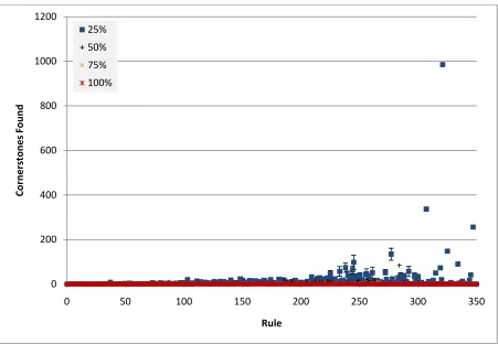
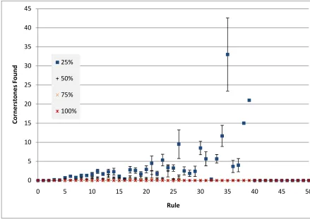
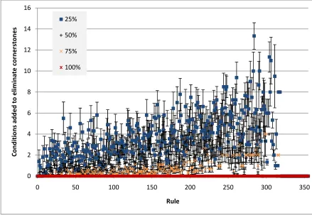
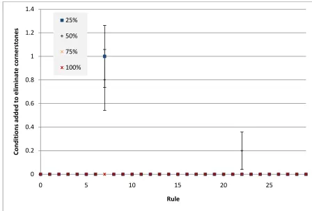
d. If there are cornerstone cases identified, continue to use more of the available conditions until they are all eliminated.

5. For each classification that is provided by a simulated expert and not provided by the system:

a. Ask the simulated expert for a rule trace.

b. Find conditions in the rule trace which are true on the current case. c. Use a number of these conditions to create a new rule to provide the

missing classification.

d. If there are cornerstone cases identified, continue to use more of the available conditions until they are all eliminated.

(13)

176

It was decided to use only one extra condition in step 4c because it has been observed in previous systems that the human expert will tend to provide very few conditions in exception rules, and this is unsurprising since they are already under the context of the parent conditions. With this approach the exception rule will only have to be as specific as necessary to eliminate the cornerstone cases being identified, and this is in line with past observations of human experts (Kang, Yoshida et al. 1997; Park, Kim et al. 2004; Bindoff, Tenni et al. 2006).

If we refer back to the expert processes described in the Literature Review and Medication Review chapters it can be seen that this algorithm does, for the main part, match the process that a human expert follows when training a knowledge base. The key differences concern the conditions used. Where a human expert will tend to use a number of conditions that spring to mind, the simulated expert will use a number of conditions from a list of pre-determined conditions depending on how specific they have been programmed to be. This is why the number of conditions used in step 5c was determined by the operational parameters of the particular run. Each experiment for each of the 10 simulated experts was run four times using 25%, 50%, 75% and 100% of the available conditions, respectively, to make their rule. This feature does to some extent simulate experts of varying “expertise”, or more correctly, specificity. The expert who used only 25% of the available rule conditions will make very general rules which tend to require a lot of refinements and the expert who uses 100% of the available conditions making very specific rules which will never need a refinement. A similar approach has been used in previous simulated expert studies (Kang 1995).

(14)

177

same feature could be modelled into the simulated expert system quite easily by imposing a random chance that the simulated expert would skip a classification; however this data would be of no relevance. The rate of error introduced would presumably be quite similar to the rate which had been coded into the system, and there would be no insight to be gained from this information. As such it is thought to be better in this situation to simply allow the simulated expert trained system to be infallible, always performing with 100% accuracy compared to the simulated experts up to the last evaluated case. Furthermore, to ensure this is the case the fool-proof method of using all previously seen cases as potential cornerstone cases is used in this study. Kang has previously demonstrated that the introduction of errors by using the less computationally intensive “past cases used to create a rule” approach to cornerstone cases is only very slight (Kang 1995), but the benefits of this approach computationally are typically very limited, since the increased cost involved in ensuring no duplicate cornerstone cases are created cancels out much of the benefit of having fewer cornerstone cases, although a well thought out indexing strategy can improve this. Further to this, since Kang already demonstrated that the introduction of errors is acceptably low, there is seen to be little reason to repeat this study here.

(15)

178

methods, and not with the problem of producing “truer” MCRDR knowledge bases since, as has already been stated, the intent here is not really to evaluate MCRDR again.

Evaluating MCRRR

The method described above, while it can be seen as an improvement in some areas on past simulated expert evaluations of MCRDR based methods, completely fails to evaluate the new MCRRR method. Since this new method is the one which is really on trial here, this is obviously an unacceptable omission.

Developing a simulated expert which is capable of creating an MCRRR knowledge base incrementally is a particularly difficult task for a variety of reasons. If nothing else, the multi-label datasets available for use are not intended to be domains in which any great level of grouping or intermediate classifications are necessary, and they are certainly not configuration or planning style problems.

Of more serious concern, however, is the simple fact that in order to produce a rule based on an existing classification which made any sense whatsoever it would be necessary for the simulated expert system to determine that there is an overlap in conditions between one classification and another, or a general trend would need to be evident that cases with a particular classification tended to have some other classification present. Doing this incrementally is seen to be challenging, since for the first approach once the system is aware that a classification has a particular set of conditions which overlap those of another classification at least one of the rules has already been created, and for the second approach the cases would need to be pre-processed in order to identify the trends. Some preliminary attempt was made to perform this pre-processing, although since only highly tenuous trends could be identified it was abandoned as unsuitable, at least for the domains available. It is conceded that perhaps an approach could be developed which could perform this task successfully, however it is felt that this is a sufficiently complex and uncertain task that it falls outside the scope of this study.

(16)

179

understand the reasons behind this better it is important to refresh our understanding of the differences between MCRDR and MCRRR. An MCRDR and an MCRRR knowledge base are not inherently different, it is simply the case that an MCRRR knowledge base can do some things that an MCRDR knowledge base cannot. Specifically, it allows for rules which use the presence or non-presence of a classification as one or more of their conditions. The advantages of this are not insignificant, with the expert potentially being able to express themselves with fewer over-all conditions needed, and the system being able to determine potentially many paths to a particular classification since the classification used as a condition might be determined from one or more of many sources which carry that classification. Further to this the system will be capable of providing its own corrections to some extent, as the expert may only have to correct one incorrect classification and the system will then “realise” that since that classification is now [not] present some other classification may now apply or stop applying as the case may be, and this correction may in turn propagate further as required.

As has been discussed previously in the Multiple Classification Ripple Round Rules chapter there are multiple ways in which a rule based on a classification or classifications might be applied, but the simplest of these, and the only way which is likely to have any application on the available datasets since they are not configuration or planning style tasks, is as a grouping rule. This style of rule is one where a particular classification may be reached through multiple rules but the grouping rule is unconcerned with which of these rules fires, only that the classification is satisfied. An example of this is shown in Figure 5-2. It should be noted that the difference between this style of rule and any other rule which uses a classification as a condition is largely in the way the expert approaches it, rather than any significant technical difference.

Root – Always true

P,Q ClassA X,Y ClassA

ClassA

H ClassB

(17)

180

In order for a grouping rule to be of clear value in the context of a simulation study it must reduce the overall number of conditions necessary, as there can be no value to the simulator in terms of the rule “making more sense that way” or “better matching how I understand it” in the same way that a human expert might experience. Unfortunately the benefit in terms of a reduction in overall conditions is unlikely to be high.

Consider again the example in Figure 5-2. The alternative to expressing the rule in this way is to have two rules “If P,Q then ClassB” and “If X,Y then ClassB”, meaning four overall conditions. The example given encapsulates this same knowledge with six overall conditions, P, Q, X, Y, H and ClassA! In order for a rule of this type to even match the overall conditions of the non-grouped alternative the intermediate classification (ClassA in this case) must be used twice. It must be used three times in order to provide a reduction in the number of overall conditions. In real-world examples where the intermediate classification may be a correct classification in its own right this is of no concern and the reduction is immediate, but if the intermediate classification exists for the sole purpose of being an intermediate classification then the reductions in conditions are likely to be quite small.

With all these limitations in mind it becomes apparent that a simulated expert evaluation of MCRRR itself would be quite difficult and of questionable value. However, it is still possible to determine a rough measure of the applicability of the method to the various datasets in terms of these grouping rules.

Hindsight Conversion

(18)

181

significant advantages offered by the MCRRR approach cannot be sufficiently evaluated, but it is difficult to imagine how it might be possible to do this, particularly as the available datasets are not built from configuration or planning style tasks. It is hoped that the configuration task outlined and evaluated in the Multiple Classification Ripple Round Rules chapter was sufficient in demonstrating its more significant capabilities in these areas.

The hindsight algorithm trialled in this study is as shown in Figure 5-3. This algorithm searches the knowledge base looking for rules which have pairs of conditions in common, and clustering these into sets of overlapped rules. These sets are then ordered by the size of their sets, so the sets with the most members are considered first and the sets with fewer members are considered last. Each set is then considered for conversion into a grouping rule, which involves checking to see that enough members of the set (rules) still exist, as some or all may have been deleted by previous iterations of the algorithm. If enough members still exist then it will create a grouping rule using the pair, delete all the rules in the set, and replace them with equivalents that use the intermediate classification instead of the original pair of conditions. The resultant knowledge base should perform exactly the same as the input knowledge base in terms of classifications provided (although with the addition of intermediate classifications), and assuming the threshold is three or more should have the same or less overall conditions.

Hindsight(Graph, Thresh) {

Overlaps = findOverlaps(Graph) Overlaps = sortBySize(Overlaps)

For each overlap pair (largest set to smallest set) {

If(overlapped rules still in existence >= Thresh)

{

buildGroupingRule(Graph) removeOverlappedRules(Graph) replaceOverlappedRules(Graph) }

} }

(19)

182

To determine the applicability of these new rules to the available domains the hindsight algorithm was applied with thresholds of 3, 4 and 5 to an MCRDR knowledge base which was produced by the simulated expert system training over 100% of the available cases. The total number of conditions were measured before the hindsight algorithm was applied, as well as after applying it with the various threshold values.

5.1.3 Datasets

The study was performed using a range of multiple classification datasets which are publically available6. A selection of these datasets were chosen based on size, and attribute types, since there are some efficiency concerns when operating with very large datasets and no suitably powerful facilities were available to complete these run-times. Despite this, the list of 7 datasets shown in Table 4 could be used. Included in this table are some relevant statistics about each dataset, a one word description of the domain they are derived from, the number of instances (cases) in the dataset, the number of nominal (text) and numeric attributes in each case, and the number of labels (classifications) in the dataset. Also included are the cardinality and density, where cardinality is defined as being the average number of labels per instance in the dataset, while density is defined as being the average number of labels per instance divided by the total number of labels in the dataset (Tsoumakas and Katakis 2007).

As can be seen, there is a good mix of nominal and numeric attribute datasets, as well as datasets with large and small numbers of labels, and a broad spectrum of sizes in terms of the number of cases. It is hoped that with this selection a sufficiently representative sample can be achieved.

6

(20)

183

Table 4 The multi class datasets used, and their relevant statistics.

Attributes N am e D om ai n In st an ce s N om in al N u m er ic L ab el s C ar d in al it y D en si ty

Emotions Music 593 0 72 6 1.869 0.311 Genbase Biology 662 1186 0 27 1.252 0.046 Scene Multimedia 2407 0 294 6 1.074 0.179 Yeast Biology 2417 0 103 14 4.237 0.303 Bibtex Text 7395 1836 0 159 2.402 0.015 Enron Text 1702 1001 0 53 3.378 0.064 Medical Text 978 1449 0 45 1.245 0.028

Dataset: Emotions

The emotions dataset consists of 72 (numeric) music features for 593 songs, and categorises each song into one or more of 6 classes of emotions. This dataset was collected for a study by Trohidis et al. (Trohidis, Tsoumakas et al. 2008).

Dataset: Genbase

The genbase dataset assigns motifs to protein families. Each instance in the dataset is a genetic sequence, represented by 1186 nominal values, which can have motifs belonging to one or more protein families, which are the 27 possible labels. The dataset was collected by Diplaris et al. (Diplaris, Tsoumakas et al. 2005).

Dataset: Scene

This dataset consists of 294 numeric attributes which attempt to describe an image. Each image is classified with zero or more of 6 classifications. The dataset was collected by Boutell et al. (Boutell, Luo et al. 2004).

Dataset: Yeast

(21)

184

Dataset: Bibtex

The Bibtex dataset was released as part of an effort to add automated tag suggesting features to content added by users on the Bibsonomy website7. It was discussed and treated as a multi-label machine learning problem by Katakis et al. (Katakis, Tsoumakas et al. 2008). This is the largest dataset used in this study, and as such only 4 folds of the 4 simulated experts were applied as opposed to the 10 folds each of the other datasets were subjected to.

Dataset: Enron

The Enron dataset is a collection of 1702 email messages selected for relevance from the Enron email database which was made publically available in 20078. Each message was annotated with categorizing labels by 2 students of the Applied Natural Language Processing course at UC Berkeley.

Dataset: Medical

This dataset was released as part of a competition to develop natural language methods to intelligently allocate ICD-9-CM (International Classification of Diseases) codes to clinical free text9. It has been adjusted to include a binary true/false statement for each possible word for each instance, such that it might be more readily used in multi-label machine learning applications.

5.1.4 Results & Discussion

For each of the datasets used in the study a series of evaluations were performed, aimed at indicating the performance and characteristics of the knowledge base produced by the various simulated experts. Each evaluation is listed below, with the results for each dataset. Although there was little intention to re-evaluate the MCRDR method itself it is, in some ways, more extensively evaluated here than past offerings, since it has been tested on a wider variety of datasets, and with true multi-label simulated experts. As such, inevitably some discussion is aimed in this direction, although the intention is more to demonstrate how each dataset behaved as an MCRDR system before its eventual conversion to MCRRR using the hindsight algorithm described earlier.

7

http://www.bibsonomy.org

8

http://www-2.cs.cmu.edu/~enron/

9

(22)

185

Growth of the Knowledge Base

This evaluation seeks to demonstrate how the knowledge base developed as it was trained by the various simulated experts. This provides an insight into the size of the knowledge base, as well as its rate of growth at various stages of training, indicating how fast and how much learning the system had to do. It is anticipated that a general trend will be seen with the 100%, overly specific, expert performing uniformly badly, of course requiring more rules since all their rules are too specific (although they should experience zero misclassifications), and the 50% expert performing typically the best. The average across the 10 (or 4 in the case of bibtex) simulated experts is shown. To give some indication of the variations experienced across this range error bars are shown which indicate one quarter of a standard deviation in each direction.

(23)

Figure 5-4 Growth of the knowledge base for the bibtex dataset.

The graph seen in Figure 5-5

which produced only around 35 r

low of only around 20 rules for the 50% and 75% experts. It appears that in both

terms of growth rate and overall performance these two experts have performed

best, learning the fastest and requiring the few

case mark it is noted that the 25%, 50%, and 75% experts were all learning about

the same low rate – so they were likely to be performing similarly well by this stage, it is simply that the 50% and 75% experts reached the

The 100% expert, as expected, performed uniformly poorly.

186

Growth of the knowledge base for the bibtex dataset.

is for the emotions dataset, a fairly simple domain

which produced only around 35 rules in the worst case for the 100% expert and a

best, learning the fastest and requiring the fewest rules. However, around the 200

so they were likely to be performing similarly well by this

stage, it is simply that the 50% and 75% experts reached the proficiency sooner.

The 100% expert, as expected, performed uniformly poorly.

is for the emotions dataset, a fairly simple domain

ules in the worst case for the 100% expert and a

est rules. However, around the 200

so they were likely to be performing similarly well by this

(24)

Figure 5-5 Growth of the knowledge bases for the emotions dataset.

Figure 5-6 shows the result for the enron dataset, another relatively large and

complex dataset. The divergence between experts is far lower in this dataset, and

the system is clearly still in a state of relatively high learni

approach 1400 cases seen. This is to be expected, since this dataset consists of a

large number of nominal attributes. Despite this the familiar trend of growth for

MCRDR knowledge bases is seen, with a sharp, high rate of learning e

gradually slows down, although it is clearly still quite far from reaching a plateau

here. Again we see a common result here, with the 100% and 25% experts requiring

more rules, the 50% expert performing well, but the 75% expert performing sligh

better still.

187

Growth of the knowledge bases for the emotions dataset.

shows the result for the enron dataset, another relatively large and

the system is clearly still in a state of relatively high learning even as the experts

MCRDR knowledge bases is seen, with a sharp, high rate of learning e

more rules, the 50% expert performing well, but the 75% expert performing sligh

Growth of the knowledge bases for the emotions dataset.

shows the result for the enron dataset, another relatively large and

ng even as the experts

MCRDR knowledge bases is seen, with a sharp, high rate of learning early which

(25)

Figure 5-6 Growth of the knowledge base for the enron dataset.

Figure 5-7 is a little harder to rea

rules and most rules having only one condition. Due to this there is very little

variance between the various experts.

188

Growth of the knowledge base for the enron dataset.

is a little harder to read into, with the genbase dataset requiring very few

rules and most rules having only one condition. Due to this there is very little

variance between the various experts.

d into, with the genbase dataset requiring very few

(26)

Figure 5-7 Growth of the knowledge base for the genbase dataset.

Figure 5-8 shows the results for the medical dataset, which demonstrates quite a

high variance in performance be

worst case. Interestingly, we can see again here that the 75% expert has performed

best, but the 100% and 50% experts are only slightly behind. This suggests that

misclassifications are a significant proble

However, all the experts do have a very similar low growth rate over the last 400

cases, suggesting that once each expert had overcome their difficult hump at around

the 250 case mark they were all performing wel

189

Growth of the knowledge base for the genbase dataset.

shows the results for the medical dataset, which demonstrates quite a

high variance in performance between experts despite having only 58 rules in the

misclassifications are a significant problem in this domain with under

cases, suggesting that once each expert had overcome their difficult hump at around

the 250 case mark they were all performing well.

shows the results for the medical dataset, which demonstrates quite a

tween experts despite having only 58 rules in the

m in this domain with under-specific rules.

(27)

Figure 5-8 Growth of the knowledge base for the medical dataset.

The story told by Figure 5-9

experts clearly performing far better than the more specific experts, and the 100%

expert in particular performing very badly, requiring far

dataset is one of the numeric datasets, and also has very few possible classifications

(only 6), and it does appear that producing more general rules with fewer conditions

is a good strategy in this style of dataset. Both the 25% and

this example able to achieve a near flawless performance from around only the 400

case mark, whereas the 75% expert took a little longer and particularly the 100%

expert never achieved this performance.

190

Growth of the knowledge base for the medical dataset.

is quite different, where we see the less specific

expert in particular performing very badly, requiring far more rules. The scene

is a good strategy in this style of dataset. Both the 25% and 50% experts were in

case mark, whereas the 75% expert took a little longer and particularly the 100%

expert never achieved this performance.

is quite different, where we see the less specific

more rules. The scene

50% experts were in

(28)

Figure 5-9 Growth of the knowledge base for the

The yeast dataset is another of these numeric datasets with few potential

classifications (14). A remarkably similar story is again seen for this dataset in

Figure 5-10. Since the error bars indicate very little deviance for the 25% and 50%

experts here, we can also see that the performance of these experts was very

consistent from run to r

191

Growth of the knowledge base for the scene dataset.

. Since the error bars indicate very little deviance for the 25% and 50%

experts here, we can also see that the performance of these experts was very

consistent from run to run.

. Since the error bars indicate very little deviance for the 25% and 50%

(29)

Figure 5-10 The growth of the knowledge base for the yeast dataset.

Accuracy of the Knowledge Base

This evaluation is designed to demonstrate the performance of the various

knowledge bases produced by the various experts as the system progresses through its training. Every 20 cases an accuracy value was determined by calculating the

number of cases which had the same outputs produced by the MCRDR system

(minus duplications) as those produced by the actu

Again, the average performance across the 10 runs of the experiment is shown, with

error bars indicating a quarter of a standard deviation in each direction.

The first accuracy result is shown in

of the experts in the bibtex dataset. It is quite difficult to tell which expert achieved

the best result overall, as the variance was not high. Howeve

the 75% and 100% experts performed marginally more accurately early, but were

overtaken by the 25% and 50% experts at around the 2500 case mark with the 100%

expert performing ultimately worst. Both the 25% and 50% experts reached 10

accuracy at around the 4500th case, while the 75% and 100% experts never quite

reached it.

192

The growth of the knowledge base for the yeast dataset.

Accuracy of the Knowledge Base

This evaluation is designed to demonstrate the performance of the various

the various experts as the system progresses through

its training. Every 20 cases an accuracy value was determined by calculating the

(minus duplications) as those produced by the actual simulated expert directly.

error bars indicating a quarter of a standard deviation in each direction.

The first accuracy result is shown in Figure 5-11, which represents the performance

the best result overall, as the variance was not high. However, it does appear that

expert performing ultimately worst. Both the 25% and 50% experts reached 10

case, while the 75% and 100% experts never quite This evaluation is designed to demonstrate the performance of the various

the various experts as the system progresses through

its training. Every 20 cases an accuracy value was determined by calculating the

al simulated expert directly.

, which represents the performance

r, it does appear that

expert performing ultimately worst. Both the 25% and 50% experts reached 100%

(30)

193

Figure 5-11 The accuracy of the system relative to the simulated experts with the bibtex dataset.

Since the emotions dataset is fairly simple the 20 case evaluation period is slightly coarse, producing not quite enough data early in the system’s training period. Despite this it is clear from Figure 5-12 that the system was very quickly learning from the simulated experts in all counts, with even the 100% expert achieving 80% accuracy by the 40 case mark. Interestingly the 75% expert is the fastest learner in terms of accuracy, with their rules being sufficiently specific to reduce misclassifications, but not so overly specific that classifications are missed. However, as the system progresses each of the 25%, 50% and 75% experts reached an accuracy of 98.32% at around the same period, although the 100% expert never quite got to the same level.

50% 55% 60% 65% 70% 75% 80% 85% 90% 95% 100%

0 1000 2000 3000 4000 5000

A

cc

u

rac

y

Case

25%

50%

75%

(31)

194

Figure 5-12 The accuracy of the system relative to the simulated experts with the emotions dataset.

Figure 5-13 which shows the accuracy for the enron dataset has a generally lower

accuracy, with the 75% expert again coming out on top. Being a nominal dataset with generally few conditions on each rule it is clear that being slightly over-specific is a marginally better strategy, for fear of simply choosing too few conditions and thus causing a misclassification soon after.

0% 10% 20% 30% 40% 50% 60% 70% 80% 90% 100%

0 50 100 150 200 250 300 350 400 450

A

cc

u

rac

y

Case

25%

50%

75%

(32)

195

Figure 5-13 The accuracy of the system relative to the simulated experts with the enron dataset.

The genbase dataset, whose results are shown in Figure 5-14 is again quite unremarkable, with the 4 different experts almost perfectly mirroring each other in performance. This is not surprising, since there are very few occasions in the genbase dataset where even 2 conditions might be used, so when talking in terms of percentages the variance in the number of conditions selected cannot be high.

0% 10% 20% 30% 40% 50% 60% 70% 80% 90% 100%

0 200 400 600 800 1000 1200

A

cc

u

rac

y

Case

25%

50%

75%

(33)

196

Figure 5-14 The accuracy of the system relative to the simulated experts with the genbase dataset.

The medical dataset is more interesting, shown in Figure 5-15. Here it can be seen that again the 75% expert is the only expert which appears to perform marginally better than the rest of the pack. This appears to match quite well with the enron, and to a lesser extent the bibtex, dataset. Since the medical dataset is, on paper, quite similar to the enron and bibtex dataset (large number of classifications, nominal values) we would expect this.

0% 10% 20% 30% 40% 50% 60% 70% 80% 90% 100%

0 100 200 300 400 500

A

cc

u

rac

y

Case

25%

50%

75%

(34)

197

Figure 5-15 The accuracy of the system relative to the simulated experts with the medical dataset.

The scene datasets results, shown in Figure 5-16, again reflect our expectations of a dataset with numeric attributes and few potential classifications, with the less specific experts performing best. In this example the 25% and 50% experts perform equally best throughout the study, although the 75% expert catches them after around the 800th case. The over-specific 100% expert performs uniformly badly throughout, with consistently far lower accuracies.

0% 10% 20% 30% 40% 50% 60% 70% 80% 90% 100%

0 100 200 300 400 500 600 700

A

cc

u

rac

y

Case

25%

50%

75%

(35)

198

Figure 5-16 The accuracy of the system relative to the simulated experts with the scene dataset.

The yeast dataset, being another numeric dataset, shows a very similar set of values in Figure 5-17. The 25% and 50% experts reach 100% accuracy by the 750th case, with the 75% expert being only marginally behind, and being in the high 90th percentile before even the 200th case is seen. The other interesting feature seen again here is that the 100% expert consistently performs a step below the rest, obviously never receiving the opportunities it requires to add those last few rules which would get it to 100% relative to the simulated expert. It seems clear that in datasets with numeric attributes a more specific expert is a worse performer in terms of accuracy.

0% 10% 20% 30% 40% 50% 60% 70% 80% 90% 100%

0 200 400 600 800 1000 1200 1400 1600 1800

A

cc

u

rac

y

Case

25%

50%

75%

(36)

199

Figure 5-17 The accuracy of the system relative to the simulated experts with the yeast dataset.

Average Conditions

This result indicates the number of conditions per rule as the knowledge base progresses in its training. To make some sense of the data each data point is a representation of the average number of conditions for the past 10 rules, with error bars again indicating a quarter of a standard deviation, although in this instance the standard deviation is of the averaged period of 10, rather than the number for each instance of the expert. Through this it is possible to gain a better understanding of how many conditions the various experts are tending to use at various stages in the development of the knowledge base. Obviously the delineation between the various experts will tend to be quite clear, since the very definition of the experts is made based on what percentage of the available rule conditions they will use for their rules. However, in cases where there are very few available conditions per rule this may not always hold true.

The results of this evaluation give us a little more insight into the results we have already seen. In Figure 5-18 we see the average number of conditions for each 10 rule cluster of the bibtex dataset. The number of conditions used here are relatively quite high for nominal datasets in this study, which is probably why the performance of this dataset relative to the other nominal datasets with a large

0% 10% 20% 30% 40% 50% 60% 70% 80% 90% 100%

0 200 400 600 800 1000 1200 1400 1600 1800

A

cc

u

rac

y

Case

25%

50%

75%

(37)

200

number of classifications, enron and medical, is unusual. That is, because there are so many conditions available for these rules it is more possible for an expert to be genuinely over-specific, whereas a less specific expert is less likely to be under-specific. This result also gives us a better understanding of why the 25% and 50% experts tend to perform similarly. This is simply because they tend to use a similar number of conditions, on average, while the 75% and 100% experts are more erratic. This is of course obvious on reflection, since a 25% expert is effectively going to suffer only 25% as much variation in the number of conditions they use relative to the number of conditions available.

Figure 5-18 The average number of conditions for every 10 rule cluster in the bibtex dataset.

Shown in Figure 5-19 is a similar, if less rich, story to that of the bibtex dataset above, with the 25% and 50% expert using a very similar number of conditions while the 75% and 100% experts are much more wild in their variation.

0 1 2 3 4 5 6 7 8

0 50 100 150 200 250 300

A

v

e

rag

e

c

o

n

d

it

io

n

s

p

e

r

1

0

r

u

le

s

Rule

(38)

201

Figure 5-19 The average number of conditions for every 10 rule cluster in the emotions dataset.

Figure 5-20 reflects a somewhat different story for the enron dataset. The 25% and

50% experts do vary quite substantially here, particularly between the 175th to 280th rule period. The reason for this is that the under-specific experts were producing rules with few conditions continuously, but then were later forced to create more specific rules because their new rules were too general and caused misclassifications in cornerstone cases. This is an example where the 25% and 50% experts were being genuinely under-specific, as the experts ultimately needed to produce more refined rules in order for these rules to be accurate.

0 1 2 3 4 5 6 7

0 5 10 15 20 25 30 35 40 45 50

A

v

e

rag

e

c

o

n

d

it

io

n

s

p

e

r

1

0

r

u

le

s

Rule

25%

50%

75%

(39)

202

Figure 5-20 The average number of conditions for every 10 rule cluster in the enron dataset.

We see in Figure 5-21 the number of conditions for the genbase dataset. Clearly it is for all experts only marginally above 1 throughout the experiment. As has already been mentioned, there were very few circumstances where there was more than 1 condition available for the expert to use, and even in these circumstances there were only 2, so even the 75% expert elected to use just one, since the experts were programmed to round up if they would otherwise select zero conditions, and round down otherwise.

0 1 2 3 4 5 6 7 8 9 10

0 50 100 150 200 250 300 350

A

v

e

rag

e

c

o

n

d

it

io

n

s

p

e

r

1

0

r

u

le

s

Rule

(40)

203

Figure 5-21 The average number of conditions for every 10 rule cluster in the genbase dataset.

Figure 5-22 shows the conditions for the medical dataset, and bears similarities to

the bibtex dataset in terms of pattern, with the 25% and 50% experts being relatively intertwined while the 75% and 100% experts show more variation. However, since the medical dataset has on average a fewer number of conditions available the differences are not quite as significant as were seen for that dataset.

0 0.2 0.4 0.6 0.8 1 1.2 1.4

0 5 10 15 20 25

A

v

e

rag

e

c

o

n

d

it

io

n

s

p

e

r

1

0

r

u

le

s

Rule

(41)

204

Figure 5-22 The average number of conditions for every 10 rule cluster in the medical dataset.

Figure 5-23 which shows the data for the scene dataset, and Figure 5-24 which

shows data for the yeast dataset, are both perfect examples of where being less specific pays off. With the very low number of possible classifications and the reasonably high number of potential conditions per rule, the 25% and 50% experts are able to vastly outperform the more specific experts using less conditions to create fewer rules in far less time and performing better as a result. The instances where 0 conditions per rule are shown on the graph actually indicate periods in which no new rules were created.

0 1 2 3 4 5 6

0 10 20 30 40 50 60

A

v

e

rag

e

c

o

n

d

it

io

n

s

p

e

r

1

0

r

u

le

s

Rule

(42)

205

Figure 5-23 The average number of conditions for every 10 rule cluster in the scene dataset.

Figure 5-24 The average number of conditions for every 10 rule cluster in the yeast dataset. 0 2 4 6 8 10 12

0 50 100 150 200

A v e rag e c o n d it io n s p e r 1 0 r u le s Rule 25% 50% 75% 100% 0 2 4 6 8 10 12

0 50 100 150 200 250

(43)

206

Depth of the Knowledge Base

Through this measure it is possible to get a feel for how many exceptions are being created. It is measured similarly to the conditions per rule, with the depth of each cluster of 10 rules being averaged. A depth of 1 is a new rule added to the root, while a depth of 2 indicates that the rule is an exception. As such, an averaged value of 1.5 would indicate that 5 of the last 10 rules were new rules, while 5 were exceptions. The error bars again indicate a quarter of a standard deviation in each direction, although in this context it is a standard deviation of the average across the period of 10 rules, as it was for the conditions per rule.

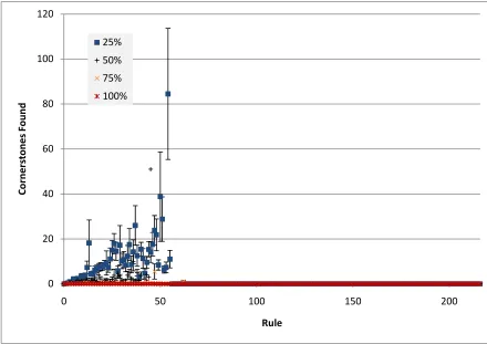
Figure 5-25 shows the average depth for each cluster of 10 rules in the bibtex

dataset, and is an example of what we might expect to see for this evaluation. It is clear that the 25% expert makes more exceptions even than the 50% expert who makes far more than the 75%, and of course the 100% expert never makes any. The other trait is of course that the number of exceptions increases as the system is trained, although at a faster rate for the less specific experts.

Figure 5-25 The average depth for every cluster of 10 rules for the bibtex dataset.

Figure 5-26 reflects a similar story for the emotions dataset, although with far

fewer examples to identify it from. It is otherwise fairly unremarkable. 1

1.1 1.2 1.3 1.4 1.5 1.6 1.7 1.8 1.9 2

0 50 100 150 200

A

v

e

rag

e

d

e