Autonomous Quadrotor Control Using Convolutional Neural Networks

Rochester Institute of Technology

RIT Scholar Works

Theses

3-2019

Autonomous Quadrotor Control Using

Convolutional Neural Networks

Amer Mahdy Hamadi

Follow this and additional works at:

https://scholarworks.rit.edu/theses

This Thesis is brought to you for free and open access by RIT Scholar Works. It has been accepted for inclusion in Theses by an authorized administrator of RIT Scholar Works. For more information, please [email protected].

Recommended Citation

1

Autonomous Quadrotor Control Using

Convolutional Neural Networks

by

Amer Mahdy Hamadi

A Thesis Submitted in Partial Fulfillment of the Requirements for the Degree of

Master of Science in Electrical Engineering

Department of Electrical Engineering and Computing Sciences

Rochester Institute of Technology -Dubai

2 Autonomous Quadrotor Control Using Convolutional Neural Networks

by

Amer Mahdy Hamadi

A Thesis Submitted in Partial Fulfillment of the Requirements for the Degree of Master of Science in Electrical Engineering Department of Electrical Engineering and Computing Sciences

Approved By:

Dr. Abdulla Ismail Date

Thesis Advisor/ Professor of Electrical Engineering- Department of Electrical Engineering and Computing

Dr. Muhieddin Amer Date

Thesis Committee member/ Professor of Electrical Engineering /Head of Department of Electrical Engineering and Computing

Dr. Jinane Al Mounsef Date

3 ACKNOWLEDGEMENTS

I would like to convey my sincere gratitude to my thesis advisor Dr. Abdulla Ismail, Professor of Electrical Engineering at Rochester Institute of Technology, for his guidance and continuous encouragement, it was great to learn from his vast knowledge and experience, and he was always available to direct me to the right track throughout this thesis.

I would also like to thank the thesis committee members Dr. Muhieddin Amer ,Head of Electrical Engineering at Rochester Institute of Technology and Dr. Jinane Al Mounsef , Assistance Professor of Electrical Engineering at Rochester Institute of Technology for their support and encouragement.

4

Declaration

I hereby declare that this thesis represents my original work and all used references are properly indicated and cited.

5

Abstract

Quadrotors are considered nowadays one of the fastest growing technologies. It is entering all fields of life making them a powerful tool to serve humanity and help in developing a better life style. It is crucial to experiment all possible ways of controlling quadrotors, starting from classical methodologies to cutting edge modern technologies to serve their purpose. In most of the times quadrotors would have combination of several technologies on board. The attitude angles and altitude control used in this thesis are based mainly on PID control which is modeled and simulated on MATLAB and Simulink. To control the quadrotor behavior for two different tasks, Obstacle Avoidance and Command by Hand Gesture, the use of Convolutional Neural Networks (CNN) was proposed, since this new technology had shown very impressive results in image recognition in recent years.

6

Table of Contents

Chapter1 Introduction to Quadrotors ... 12

1.1 Overview and Definitions: ... 12

1.2 QUAV Applications: ... 13

1.3 QUAV Components: ... 13

1.3.1 Sensors: ... 14

1.3.2 Brushless DC Motor: ... 17

1.3.3 Electronic Speed Controller: ... 17

1.4 Thesis Objectives: ... 18

1.5 Work Methodology: ... 18

1.6 Thesis Outline: ... 18

Chapter 2 Quadrotor Modeling ... 19

2.1 Quadrotor Configuration: ... 19

2.2 General Moments and Forces ... 20

2.3 Quadrotor Equations of Motion ... 22

2.4 Simulation ... 24

Chapter 3 PID Control of Quadrotor ... 27

3.1 PID Controller ... 27

3.2 PID Simulation and Results: ... 29

3.3 Results Discussion ... 34

Chapter 4 Control of Quadrotor Using Convolutional Neural Networks ... 35

4.1 Introduction to Neural Network ... 35

4.2 Deep Learning ... 36

4.3 Previous Work ... 37

4.4 Convolutional Neural Network ... 37

4.4.1 Convolutional Layer ... 39

4.4.2 Non Linear Activation Function ... 40

4.4.3 Pooling Layer ... 41

4.4.4 Dropout Layer ... 41

4.4.5 Classification layer ... 42

7

Chapter 5 Implementation ... 44

5.1 Controller Design and Implementation ... 44

5.2 CNN Implementation... 44

5.2.1 Obstacle Avoidance ... 44

5.2.2 Command by Hand Gesture ... 46

5.3 Setup of the test-bed (Experiment Setup) ... 48

5.4 Programming Quadrotor Behavior ... 50

5.5 Real-Time UAV Flight Experiments ... 51

Chapter 6 Conclusion and Future Works ... 53

References ... 54

Appendix A ... 56

MATLAB Code for Quadrotor Maneuvers. ... 56

Appendix B ... 57

Arduino UNO Pinout ... 57

Appendix C ... 58

8

List of Tables

Table 1.1 UAV Classification ... 13

Table 2.1 Quadrotor Parameters ... 25

Table 3.1 Response of Closed Loop system to PID gains ... 28

Table 3.2 Comparison of unit step responses for the QUAV PID controllers ... 34

Table 4.1 List of different CNN topologies that participated in ImageNet challenge ... 43

Table 5.1 Obstacle Avoidance CNN Layers ... 45

Table 5.2 The Confusion Matrix (ConfMat) ... 45

Table 5.3 A comparison before and after modification of AlexNet layers ... 47

9

List of Figures

Figure 1.1: Different types of recent UAVs ... 12

Figure1.2: Typical Quadrotor Components [7] ... 14

Figure 1.3: Flight Controller for Quadrotor with Sensors..[8] ... 15

Figure 1.4: Accelerometer and Gyroscope..[7] ... 15

Figure 1.5: Camera with Video Signal Transmitter ..[7] ... 16

Figure 1.6: Outrunner 1200 BL-DC Motor upper and bottom view ... 17

Figure 2.1: Pitch, roll and yaw torques of the quad-rotor ... 19

Figure 2.2: Quadrotor motion description- the arrow width is proportional to rotor speed [5] ... 20

Figure 2.3: The angular and translations subsystems ... 24

Figure 2.4: System model using Simulink ... 25

Figure 2.5: Angular Subsystem ... 26

Figure 2.6: Linear Translations Subsystem ... 26

Figure 3.1: Closed Loop PID control Block Diagram ... 27

Figure 3.2: System with PID controllers ... 29

Figure 3.3: The Roll φ controller ... 30

Figure 3.4: System step response for the Roll φ controller ... 30

Figure 3.5: The Pitch θ controller ... 31

Figure 3.6: System step response for the Pitch θ controller ... 31

Figure 3.7: The Yaw ψ controller ... 32

Figure 3.8: System step response for the Yaw ψ controller... 32

Figure 3.9: The Altitude z controller ... 33

10

Figure 3.11: Simulation for the Quadrotor in 3D space ... 34

Figure 4.1: Simple Neuron with essential components ... 35

Figure 4.2: Simple Artificial Neuron ... 35

Figure 4.3: Simple Neural Network ... 36

Figure 4.4: Deep Learning Classification ... 36

Figure 4.5: LeNet-5 architecture ... 37

Figure 4.6: Convolutional Neural Network learning representation ... 38

Figure 4.7: Left : Classic 3 layer Neural Network. Right: A CNN layer that arrange its neurons in three dimensions (width, height , depth). ... 38

Figure 4.8: A mathematical representation of the convolution operation ... 39

Figure 4.9: The activation function ... 40

Figure 4.10: Max and Average Pooling Layer ... 41

Figure 4.11: Dropout representation [17] ... 41

Figure 4.12: The Softmax layer ... 42

Figure 5.1: Two sample pictures for Left and Right classes each is 32x32 pixels ... 44

Figure 5.2 AlexNet Deep Neural Network ... 46

Figure 5.3: Left and Right gesture command images added to the dataset ... 46

Figure 5.4: Filters of the first convolutional layer ... 48

Figure 5.5: System block diagram ... 48

Figure 5.6: The Interface Circuit ... 49

Figure 5.7: CNN classify obstacle orientation and QUAV act to avoid it ... 50

Figure 5.8: CNN network recognizes a gesture and Quadrotor responds accordingly. ... 50

11

List of Symbols

A propeller disk area

Ac fuselage area

b thrust factor

c propeller chord

C propulsion group cost factor

d drag factor

g acceleration due to gravity

h vertical distance: Propeller center to CoG

H hub force

Ixx,yy,zz inertia moments

Jr rotor inertia

l horizontal distance: propeller center to CoG

m overall mass

Q drag moment

Rm rolling moment

T thrust force

U control inputs

x,y,z position in body coordinate frame X,Y,Z position in earth coordinate frame

θ pitch angle

ρ air density

φ roll angle

ψ yaw angle

Ω propeller angular rate

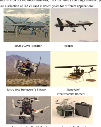
12 2000’s UAVs Predator Reaper

Micro UAV Honeywell’s T-Hawk Nano UAV PrexDynamics Hornet3

Quadrotor AsecTec “Pelican” AeryonLabs “Scout”

Figure 1.1: Different types of recent UAVs

Chapter1 Introduction to Quadrotors

1.1 Overview and Definitions:

UAV (Unmanned Aerial Vehicle) is an aircraft without a pilot, depending mainly on autonomous or remote flight control, this system is used in recent years in many civil and military applications, providing many advantages over manned systems such as reduced cost, no risk on crew for hazardous missions, maneuverability and long endurance [4]. Figure 1.1 shows a selection of UAVs used in recent years for different applications.

13

UAVs can be classified according to size , range, altitude or number of rotors . Table 1.1 shows the possible classification of UAV.

Table 1.1 UAV Classification

UAV

Size

Range

Altitude

Wing Configuration

No. of Rotors

(MAV) Close range High Altitude Long Endurance HALE Fixed Wing Sigle Rotor

Mini

(MUAV) Short range

Medium Altitude Long Endurance

MALE Flapping wing Multi rotors

Nano

(NAV) Medium Range Endurance Blimps

QUAV is a Quadrotor UAV that is lifted and propelled by four rotors [1].It is considered a benchmark research platform because of its high maneuverability and simple mechanical structure. However, the control design for this type of systems is a complex task.

1.2 QUAV Applications:

QUAV has a wide range of applications, including the following [4]:

 Security fields (supervision of aerial space, urban traffic),

 Natural risks management of supervision of active volcanoes and of environment (measuring air pollution, supervision of forests),

 Intervention in hostile environments (radioactive atmospheres, removal of mines without human intervention),

 Monitoring and management of ground installations (dams, lines with high tension, pipelines),

 Agriculture (detection and treatment of infested cultivations), and aerial shooting in the production of movies.

 Light shows around the world, including recently in 2018’s Winter Olympicsopening ceremony [6].

1.3 QUAV Components:

14

Figure1.2: Typical Quadrotor Components [7]

1.3.1 Sensors:

To design an aerial autonomous robot that can perform specific tasks, and to have the drone interact with surrounding environment fast and accurately, an effective selection of the sensors need to be done. The choice of the sensing device depends on the task required to be

15

Figure 1.4: Accelerometer and Gyroscope..[7] Figure 1.3: Flight Controller for Quadrotor with Sensors..[8]

• Gyroscope: it measures the angular velocity of a system Microchip-packaged Micro Electro Mechanical Systems (MEMS) gyroscopes are commonly used for the stabilization,

• Accelerometer: it measures the linear acceleration, (see Figure 1.4) .

16 Fig 8 Magnetometer/Compass..[7]

Figure 1.5: Camera with Video Signal Transmitter ..[7]

• Inertial Measurement Unit (IMU): it measures and reports on a craft’s velocity, orientation, and gravitational forces, using a combination of accelerometers, gyroscopes and a compass

• Global Positioning System (GPS): it provide the absolute location anywhere on Earth using four or more GPS satellites.

• Laser Range Finder (LRF): it uses a laser beam to determine the distance to an object

• Ultrasonic Sensor: it detects the distance of an object by sending high frequency sound wave and measuring the time required for the echo detected by special sensors, and determine the distance accordingly.

• Infrared Sensor: it uses the same concept of ultrasound sensor but using infrared waves and used for shorter distances.

17

Figure 1.6: Outrunner 1200 BL-DC Motor upper and bottom view

1.3.2 Brushless DC Motor:

The BL-DC motor is a permanent magnet synchronous motor where the magnetic fields are uniformly distributed in the air gap. A permanent magnet field excitation is used in rotor instead of electromagnets. The BL-DC motor replaces the mechanical commutator by using an electronic commutator in the form of an inverter in the ESC, allowing the armature of the machine to be on the stator, as in Figure. 7 [4].

1.3.3 Electronic Speed Controller:

18

1.4 Thesis Objectives:

The objectives of this thesis are to have thorough study of the quadrotor system, understand all factors that affect the system control, modeling the system to represent it mathematically, analyze the response for different input signals and design the appropriate controller to achieve system stability. Quadrotor control using neural network is proposed with two tasks. First is to avoid obstacles and the second task is to command the quadrotor with hand gesture. To achieve these objectives, a large library of data set is acquired, then building and training the neural network to classify different classes. This classification output sends commands to the Quadrotor accordingly, hence a microcontroller with appropriate interface circuit is designed and implemented. The two tasks are done in two different neural network architectures and their performances are examined.

1.5 Work Methodology:

The methodology includes selecting a mathematical model of the quadrotors, using state variable method, simulate the system using MATLAB to understand it thoroughly, looking for a set of specifications for good performance, design controllers using conventional PID, utilizing the CNN network to implement two different tasks and coming up with conclusions.

1.6 Thesis Outline:

Chapter 1 provides an overview of the UAV and classification and a general concept of Quadrotors configuration and components. Chapter 2 discusses the modeling of a Quadrotor. Chapter 3 gives a basic definition for PID controller, then the design of appropriate controllers for the system is determined. Chapter 4 discusses the Convolutional Neural Network

techniques and layers and shows case study examples. Chapter 5 discusses the CNN

19

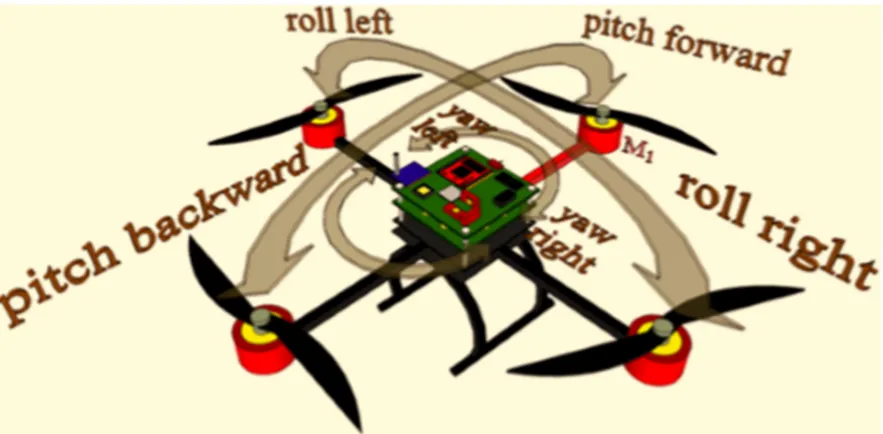
Figure 2.1: Pitch, roll and yaw torques of the quad-rotor

Chapter 2 Quadrotor Modeling

2.1 Quadrotor Configuration:

Quadrotors in general use two pairs of identical propellers (1,3) and (2,4) as described in Figure 2.1. Two turn clockwise (CW) and two counterclockwise (CCW). To achieve control of quadrotor , an independent variation of the speed of each rotor is used [4].

The basic Quadrotor motion is defined by using Euler angles yaw ψ, pitch θ, roll φ and vertical motion z. The motion in these directions can be achieved by having the following propeller speed variation [1]:

 Changing the speed of all propellers at the same time will generate vertical z motion.

 Changing 2 and 4 propellers conversely will create a roll φ rotation.

 Changing 1 and 3 propellers conversely will create a pitch θ rotation.

20

Figure 2.2: Quadrotor motion description- the arrow width is proportional to rotor speed [5]

(a)Yaw CCW (b)Yaw CW (c) Vertical Up (d)Roll CW (e) Pitch CCW

(f)Pitch CW (g) Vertical Down (h)Roll CCW

2.2 General Moments and Forces

The forces and moments responsible of Quadrotor motion are listed below[9]:

Rolling Moments

body gyro effect

propeller gyro effect

roll actuators action

hub moment due to sideward flight

21 Pitching Moments

body gyro effect

propeller gyro effect

pitch actuators action

hub moment due to forward flight

rolling moment due to sideward flight

Yawing Moments

body gyro effect

inertial counter-torque

counter-torque unbalance

hub force unbalance in forward flight

hub force unbalance in sideward flight

Forces Along z Axis

actuators action

weight

Forces Along x Axis

actuators action

hub force in x axis

friction

Forces Along y Axis

actuators action

22

2.3 Quadrotor Equations of Motion

The equations of motion of quadrotor are derived below using all the forces and moments listed in section 2.2

In this thesis, general assumptions were made that the quadrotor model is simplified as a rigid body with its structure distributed symmetrically around the center of mass. To simplify the model, the hub forces and rolling moments were neglected. The system state-space form can be written as 𝑋̇ = 𝑓(X,U) with U inputs vector and X state vector as follows [9]:

State vector

(2.1)

23

Where the inputs are:

From above we obtain after simplification:

(2.3)

(2.4)

(2.5)

24

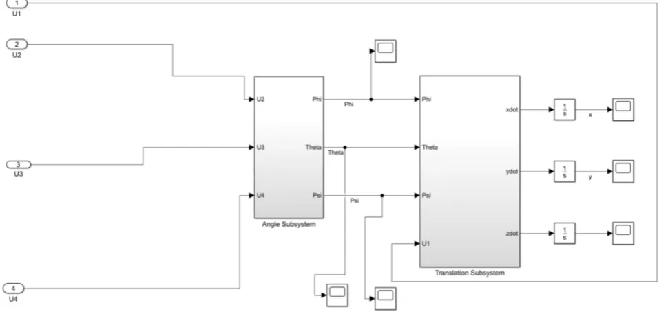
Ideally, the system derived from the above equation consists of two subsystems, the Angular and Translation subsystems as shown in Figure 2.3.

Figure 2.3: The angular and translations subsystems

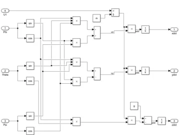
2.4 Simulation

In order to validate the presented system equations, a simulation environment is created under Simulink. The simulation is based on the full nonlinear model of the quadrotor presented by the

25

Figure 2.4: System model using Simulink

The Quadrotor parameters used in the simulation are summarized in Table 2.1 [9]

Table 2.1 Quadrotor Parameters

Parameter Value Parameter Value

Ixx 0.0075 a1 (Iyy-Izz)/Ixx

Iyy 0.0075 a2 Jr/Ixx

Izz 0.013 a3 (Izz-Ixx)/Iyy

l 0.23 a4 Jr/Iyy

d 7.50*10^(-7) a5 (Ixx-Iyy)/Izz

Jr 6.5*10^(-5) b1 l/Ixx

g 9.81 b2 l/Iyy

m 0.65 b3 1/Izz

b 3.13*10^(-5) la 0.23

26

Figure 2.5: Angular Subsystem

27

Chapter 3 PID Control of Quadrotor

3.1 PID Controller

PID controller is considered by far the most predominant form of control loop feedback mechanism used in industrial automation because of its remarkable effectiveness and implementation simplicity.

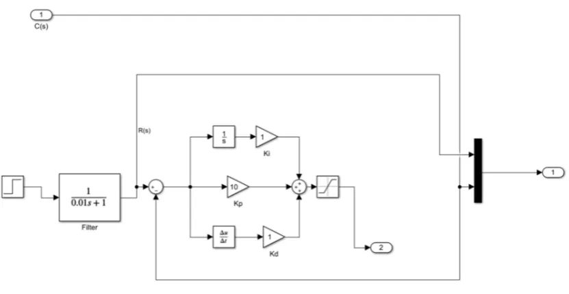
A basic PID control mechanism is shown in Figure 3.1.The error e(t) is calculated as the difference between a measured process variable and a desired set-point. The controller minimizes the error by the use of a manipulated variable. The PID controller process involves three separate constant parameters and is respectively: the proportional, the integral and the derivative values, denoted by P, I, D [2].

The closed loop system with the three objectives to be met is achieved by tuning the control parameters:

1. System stability

2. Fast transient response e.g. rise time, overshoot, and settling time.

3. Acceptable steady state accuracy [11].

Figure 3.1: Closed Loop PID control Block Diagram

The transfer function of the PID controller is given by:

28

The tracking error (e) represents the difference between the desired input value (r) and the actual output (Y). This error signal (e) will be sent to the PID controller, and the controller calculates both the derivative and the integral of this signal. The signal (u) just after the controller is now equal to the proportional gain (Kp) times the magnitude of the error plus the integral gain (Ki) times the integral of the error plus the derivative gain (Kd ) times the derivative of the error.

u = K

e + K

∫e dt + K

This signal (u ) will be sent to the plant, and the new output ( Y) will be acquired. This output ( Y) will be sent back to the sensor again to get the new error signal (e). The controller takes this new error signal and calculates its derivative and it is integral again. This process is repeated on and on again.

A proportional controller (Kp) will reduce the rise time and reduce, but not eliminate, the steady-state error. An integral control (Ki) eliminates the steady-state error, but it may worsen the transient response. While a derivative control (Kd) will increase the stability of the system, reduce the overshoot, and improve the transient response. The effect of each controller Kp,Ki,Kd on the system are summarized in Table 3.1.

Table 3.1 Response of Closed Loop system to PID gains

Tuning methods for PID controllers can be categorized according to their usage and nature. Standard tuning methods are the Analytical methods, Frequency response (such as loop-shaping), Heuristic methods (such as Z-N tuning rule, fuzzy logic and neural networks), Optimization methods and Adaptive tuning methods.

CL RESPONSE RISE TIME OVERSHO OT SETTLING TIME S-S ERROR

Kp Decrease Increase Small Change Decrease

Ki Decrease Increase Increase Eliminate

Kd _ChangeSmall Decrease Decrease Small _Change

29

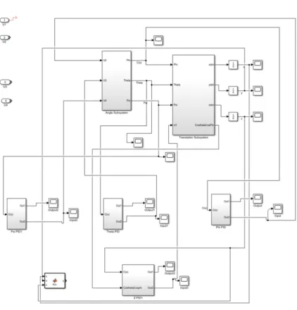
3.2 PID Simulation and Results:

Four PID controllers are added to the system to control roll, pitch, yaw and altitude as shown in Figure 3.2.

30

Roll Controller

The Roll φcontroller is implemented as shown in Figure 3.3

Figure 3.3: The Roll φ controller

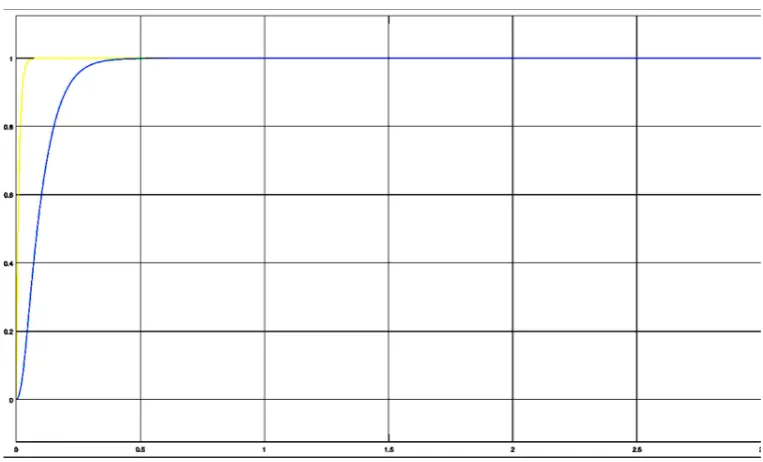
After tuning the values of Kp=9 , Ki=0, Kd=1 the system step response is shown in Figure 3.4.

31

Pitch Controller

The Pitch θ controller is implemented as shown in Figure 3.5

Figure 3.5: The Pitch θ controller

Tuning Kp=10 , Ki=1, Kd=1 the system step response is shown in Figure 3.6.

32

Yaw Controller

The Yaw ψ controller can be implemented as shown in Figure 3.7

Figure 3.7: The Yaw ψ controller

Tuning Kp=5 , Ki=5, Kd=1 the system step response is shown in Figure 3.8.

33

Altitude Controller

The Altitude z controller can be implemented as shown in Figure 3.9.

Figure 3.9: The Altitude z controller

Tuning Kp=150 , Ki=20, Kd=100 the step response is shown in Figure 3.10.

34

3.3 Results Discussion

The results from above the response figures are summarized in Table 3.2.

Table 3.2 Comparison of unit step responses for the QUAV PID controllers

Roll φ Pitch θ Yaw ψ Altitude z

Rise Time(sec) 0.4 0.3 0.4 1.7

Settling Time(sec) 0.45 0.35 2.5 5

Peak Overshoot (%) 0 0 4 8

Steady State Error(sec) 0 0 0 4

Examining Table 3.2 shows us a good understanding of the PID control response. The rise time required for Altitude is much longer than for the attitude angles which is obvious in real flight for the Quadrotor, where changing the altitude and reaching settling time is taking more time than merely changing the yaw angle, for example, which would take less than a second. However unlike the attitude angles, the Altitude control has a steady state error and noticeable 8% Overshoot.

The Rise and Settling times for unit step response for the Roll and Pitch angles were all under 0.5 second and have zero overshoot and Steady State Error, while the Yaw angle required more settling time and the response suffered from Peak Overshoot of 4%.

The PID control is proposed to stabilize the QUAV and according to the above response results and comparing to the previous work of the references [9], [3], the proposed strategy is successfully applied and the controllers are performing satisfactorily.

Since the system step response is not illustrating the Quadrotor behavior in real flight and to have a better idea of the response to multiple inputs at the same time, a 3-Dimentional visualization of the Quadrotor, as a simulation is running, is implemented as shown in Figure 3.11. In this system the Quadrotor is following an arbitrary trajectory of a ramp z input and a sinusoidal signal in pitch angle.

35

Chapter 4 Control of Quadrotor Using Convolutional

Neural Networks

4.1 Introduction to Neural Network

A Neural Network, is an interconnected processing nodes based on the structure and functions of the biological brain neural networks. Figure 4.1 shows a simple neuron cell where the input is derived from other cells through junctions called Synapses, then after processing the information an output is

transmitted through the Axon to other cells [10].

Figure 4.1: Simple Neuron with essential components

The artificial equivalent for this cell is the neural node in a neural network as shown in Figure 4.2 where Synapses are modeled with weights to be multiplied by the input values, and then added together in the node to compare it in this example to a threshold and send a zero or one according to the

comparison result.

Figure 4.2: Simple Artificial Neuron

36

Figure 4.3: Simple Neural Network

4.2 Deep Learning

Deep Learning is a subsection of Machine Learning, which in turn is a subset of Artificial Intelligence. One can define Artificial Intelligence (AI) as the study that enables machines to carry out tasks that normally require human intelligence. Many other fields of research fall within AI such as expert systems, genetic algorithms, etc. Machine Learning is a type of AI (figure 4.4) that makes computers capable of learning without being explicitly programmed step by step and does predictions on data.

37

Deep learning has several architecture types for example the Convolutional Neural Network (CNN) used for 2D recognition such as images, Recurrent Neural Network (RNN) for Voice recognition, Deep/Restricted Boltzmann Machines RBM and Long Short Term Memory networks LSTMs.

4.3 Previous Work

Hubel and Wiesel [11] are considered the pioneers in modeling cells and can learn invariant features inspired by the visual cortex of a cat, where some neurons fire only when exposed to edges in certain direction, and the multi-layered perceptron (MLP) architecture is consisting of alternating simple and complex layers introducing the basis of CNNs. Fukushima [12] followed a similar architectural pattern and titled the work Neocognition [13]. In 1998, using the similar feature extraction method

,Neocognition implemented a successful use of CNN to use in handwritten characters recognition. Figure 4.5 illustrates the architecture employed by LeCun et al. [13]. The network name was LeNet-5. It had 6-layers with 3 convolutional layers, two pooling and one fully connected layer at the end.

Figure 4.5: LeNet-5 architecture

For many years CNN was not used because of the high computational cost. While shallow machine learning couldn’t handle larger more complex images and problems, recently, in 2012, CNN emerged again accomplishing a very impressive performance and much lower error rates, supported by the availability of high-end computational hardware and the extraordinary success achieved by

Convolutional Neural Networks CNN in ImageNet Competition [14]. The network name is AlexNet after the name of the paper’s author Alex Krizhevsky.

4.4 Convolutional Neural Network

38

Initial layers capture low level features such as edges and corners, then followed by middle layers that capture mid-level features like object parts, and the last layer captures high level-class specific features such as an object model and a face detector as shown in Figure 4.6.

Figure 4.6: Convolutional Neural Network learning representation

A classic Convolutional Neural Network consists of a multiple convolutional and fully connected layers, in which most of the operations are executed; pooling layers that are used to evade over-fitting; a classification layer and to classify final results into classes. Each layer in the CNN comprises of 3D volumes of neurons, with width, height, and depth as shown in Figure 4.7[15].

39

4.4.1 Convolutional Layer

Most of the operations are done by the convolutional layer, which is the execution of a convolution operation involving 3 dimensional multiply accumulate (MACC). A filter/kernel of weights is multiplied by the respective regions in the input image and the weighted inputs are summed together with a bias which value is usually one as shown in Figure 4.8 [15].

Figure 4.8: A mathematical representation of the convolution operation

The convolutional layer receives the images as 3 dimensional arrays with height , width and no. of color channels of the images.

The output is also a 3D array yj as described in the equation:

yj = bj + ∑i Kij∗ xi

where xi is the input to the layers, i is the filter number, Kij is the kernel , bj is the bias and * indicates

the convolution operator.

The size of the output can be calculated as shown in Equation:

𝑂𝑢𝑡𝑝𝑢𝑡𝑠𝑖𝑧𝑒 =(𝐼𝑛𝑝𝑢𝑡𝑤𝑖𝑑𝑡ℎ−𝐹𝑖𝑙𝑡𝑒𝑟𝑠𝑖𝑧𝑒+2× 𝑃𝑎𝑑𝑑𝑖𝑛𝑔) /𝑆𝑡𝑟𝑖𝑑𝑒 + 1

where the stride is the slide rate at which the filter moves to the right at a time (usually one pixel) , and padding is adding extra pixels to the border of the input to control size of the output and preserve the useful information.

(4.1)

40

4.4.2 Non Linear Activation Function

The activation function is applied to each pixel to discard any unnecessary information. There are several types of activation functions used in this layer. The most common ones are:

The sigmoid function :

sig(x) = 1 / (1 + e-x₎

The Hyperbolic function

tanh(x) = (e2x _{- 1) / (e}2x _{+ 1)}

The Rectified Linear Unit (ReLU):

f(x) = max(0, x)

Figure 4.9: The activation function

Most deep learning networks nowadays are using ReLU-max(0, x), because it converges faster in training [14], While other functions saturate, the ReLU guarantees a positive output for any positive input.

(4.3)

(4.4)

41

4.4.3 Pooling Layer

The pooling Layer’s main function is to reduce the size of the propagated input without losing any important information, keeps the relevant information and removes unnecessary ones [16] , which makes the Pooling layer reduce the sensitivity of activations and increase the robustness against noise.

There are two common methods of pooling :max pooling and average pooling. In max pooling, the maximum value in the pooling filter is selected and other values are dropped, while in the average pooling the average value is calculated and passed to the next layer as shown in Figure 4.10 [15].

Figure 4.10: Max and Average Pooling Layer

4.4.4 Dropout Layer

A technique is used to reduce the over-fitting problem where a very precise mapping increases the error while testing. To combat this problem, a random percentage of neurons are tuned off during the training phase, forcing the network to be redundant. In the validation and testing, all the neurons are used again (Figure 4.11). The technique has excellent results [17].

(a) Standard Neural Network (b) After applying dropout

42

4.4.5 Classification layer

The main functionality for this layer is to categorize the output into specific classes; the most common function used is Softmax, which converts scores in the preceding layers to a probability value that indicates the confidence level of the selected class as shown in Figure 4.12.

Figure 4.12: The Softmax layer

4.5 Case Studies

The Following is a description of the main CNNs,

1) LeNet [13] 1998- developed by YannLeCun , is the real pioneer in the applications of CNNs, which were used to read zip codes, digits, etc.

43

second runner-up achieved 26.2% top-5 error. The training was done by two GTX580 GPUs for five to six days. The architecture is described in further details in Subsection 5.2.2 .

3) ZF Net [18]2013 – The winner of ILSVRC 2013 was a CNN from Matthew Zeiler and

Rob Fergus, which is known as the ZFNet. This network was more of a fine tuning to the previous

AlexNet architecture. ZF Net was trained on only 1.3 million images while AlexNet was trained on 15 million images. The training was done on a GTX580 GPU for twelve days.

4) GoogLeNet [19] – It is the ILSVRC 2014 winner with a top5 error rate of 6.7%. This paper

introduced a new module called the inception which uses average pooling instead of fully connected layers Net, which helps to reduce a large number of parameters. There are also several follow-up versions to GoogLeNet, most recently Inception-v7 [20]. It was trained on a number of high-end GPUs for a week.

5) VGGNet [21] – It is the second best entry in ILSVRC 2014. This paper’s main contribution was proving that the network depth has a critical role in the network performance. The network has 16 CONV/FC layers and features.

6) ResNet [22] – Microsoft Residual Network is the ILSVRC 2015 winner developed by Kaiming He et al. Like GoogleNet, the architecture removes the fully connected layers at the end of the network. The error rate was 3.6%. It has 152 layers ”Ultra Deep” , and was trained on 8 GPU machines for two to three weeks.

44

Chapter 5 Implementation

5.1 Controller Design and Implementation

The main objective of this thesis is to experiment the combination of PID controller and Convolutional Neural Network to achieve autonomous flight of quadrotors, and utilize the same setup to achieve different tasks. Human eyes are crucial perception sensors for the surrounding environment. The depth awareness is created by merging the two images coming from human being eyes in the visual cortex. Although the depth is a very important information but there are many species which survive efficiently using two dimensional images, leaving the brain with the image analysis burden. Following the preceding logic, a single camera is used in this research to give feedback to the CNN. No additional sensor is used to estimate depth or sense obstacles. In addition no filter or image segmentation is used. The raw image is fed directly to the CNN.

5.2 CNN Implementation

In the last six years, deep learning has massively altered the domain of machine learning, computer vision, pattern recognition, robotics etc. It has been proved that deep learning is capable of achieving better detection results than traditional techniques, because of its filtering through its multiple layers [23].

In this thesis, two tasks were selected using the same setup:

 Obstacle avoidance using 15 layers and 32x32x3 pixel images.

 Command by gesture, which uses Transfer Deep Learning from AlexNet, with 25 layers and

227x227x3 images . 5.2.1 Obstacle Avoidance

A dataset is made of 4 classes, where each class has 130 images of the obstacle position inside the image frame (right , left, up, down), Figure 5.1 shows a sample of two class shots (left and right) for this project.

45

The first convolutional layer was chosen to have to dimension of 32x32x3 for the sake of computational efficiency. Therefore, the input images were resized accordingly. The training and validation images were chosen randomly to be 80% and 20% of the total images respectively.

The second layer is the pooling layer that decreases the dimensions of the following layers, that are alternating with the pooling. There are three convolutional layers on the second fifth and ninth layers and the last layer is Softmax layer for classification. The number of filters used in the pooling layers and the dimensions of each layer are detailed in Table 5.1.

Table 5.1 Obstacle Avoidance CNN Layers

# Layer name Description

1 'imageinput' Image Input

2 'conv_1' Convolution

3 'maxpool' Max Pooling

4 'relu_1' ReLU

5 'conv_2' Convolution

6 'relu_2' ReLU

7 'avgpool_1' Average Pooling

8 'conv_3' Convolution

9 'relu_3' ReLU

10 'avgpool_2' Average

11 'fc_1' Fully Connected

12 'relu_4' ReLU

13 'fc_2' Fully Connected

14 'softmax' Softmax

15 'classoutput' Classification Output

Results:

The CNN network was trained with hundreds of obstacles photos with different orientations. The success rate is measured with a matrix known as Confusion Matrix, which is shown in Table 5.2. The results are obtained from training and validation phases. The training required 20.83 seconds on the GPU. The mean accuracy rate was 75%.

Table 5.2 The Confusion Matrix (ConfMat)

Up Down Left Right

Up 0.6364 0.3636 0 0

Down 0 0.7714 0.1429 0.0857

Left 0 0.1351 0.8198 0.0541

46

5.2.2 Command by Hand Gesture

The second CNN experiment implemented in this thesis uses Transfer Learning. The main drawback of CNNs is the requirement of vast training datasets, which need long computational time and special hardware during training. Yet, testing time is very less, which qualify it to meet the requirements of real time applications. To defy the requirement for large datasets, a concept called Transfer Learning is usually used.

Transfer learning is the technique of using a pre-trained model with the weights and parameters of a network that has been trained on a large (AlexNet in this thesis) and since the images are somewhat similar in nature, a “fine-tuning” is done for the model with the new dataset. The original AlexNet Network is shown in Figure 5.2.

Figure 5.2 AlexNet Deep Neural Network

The fine tuning is done by replacing only the last layers with the new classifier and keeps all of the other pre-trained layers which will act as a feature extractor, and then re-train the network normally. In our case the 23rd _{layer is replaced because AlexNet has 1000 neurons in it to classify 1000 objects,} while the requirement here is only five gesture images for Up, Down, Left, Right and Stop. Figure 5.3 shows two examples of the gesture’s control images used in this experiment.

47

The 25th _{layer will also be replaced with a new layer that classifies the five gestures above. The layers} comparison before and after modification are shown in Table 5.3.

Table 5.3 A comparison before and after modification of AlexNet layers

# Name AlexNet Modified

1 'data' Image Input Image Input

2 'conv1' Convolution Convolution

3 'relu1' ReLU ReLU

4 'norm1' Cross channel Cross channel

5 'pool1' Max Pooling Max Pooling

6 'conv2' Convolution Convolution

7 'relu2' ReLU ReLU

8 'norm2' Cross channel Cross channel

9 'pool2' Max Pooling Max Pooling

10 'conv3' Convolution Convolution

11 'relu3' ReLU ReLU

12 'conv4' Convolution Convolution

13 'relu4' ReLU ReLU

14 'conv5' Convolution Convolution

15 'relu5' ReLU ReLU

16 'pool5' Max Pooling Max Pooling

17 'fc6' Fully Connected Fully Connected

18 'relu6' ReLU ReLU

19 'drop6' Dropout 50% Dropout 50%

20 'fc7' Fully Connected Fully Connected

21 'relu7' ReLU ReLU

22 'drop7' Dropout 50% Dropout 50%

23 'fc8' Fully Connected layer (1000

neurons) Fully Connected layer (5 neurons)

24 'prob' Softmax Softmax

25 'output' Classification Output 1000 classes Classification Output 5 classes

Results:

The training using different gestures photos required 180.36 seconds on the GPU. The results obtained from training and testing phases have a mean accuracy rate equals to 98%. The accuracy is significantly greater than the 15 layer-network used in the first task, and it is proof of the robustness and flexibility of AlexNet to adapt to new tasks other than what it was initially designed for.

48

Figure 5.4: Filters of the first convolutional layer

5.3 Setup of the test-bed (Experiment Setup)

The setup is designed to have the inner loop responsible for the attitude control and typically uses a PID controller located in the quadrotor. The outer loop is responsible for the position performed by the ground station as shown in Figure 5.5.

49

The ground station is a computer with a processor Intel i7-4150U @2.60 GHz , an 8GB memory and a GPU NVIDIA Geforce 840M, dedicated 4GB memory having a capability to work with CUDA library that is required for the CNN computation. MATLAB codes are done for two different tasks,

communicating via a serial port RS232 with an Arduino microcontroller which is sending commands to the quadrotor as shown in Figure 5.6. The feedback loop is the real time video stream sent by the quadrotor onboard camera.

The Arduino ports used to control the attitude and altitude of the quadrotor are shown in Table 5.4.

Table 5.4 Arduino ports assignemnet

Arduino Port Control Action

D6 Roll Right

D11 Roll Left

D8 Hover Up

D9 Hover Down

D10 Pitch Forward

D7 Pitch Backword

An interface circuit was designed to connect the Arduino ports to the wireless controller, mainly using a photo coupler as shown in Figure5.6, to eliminate any noise interference back to Arduino and host computer. The datasheet for the photo coupler and Arduino Microcontroller are displayed in Appendix 2 and 3.

50

5.4 Programming Quadrotor Behavior

For both tasks, the quadrotor will start rising automatically to a certain elevation, then start sending the video stream to the host computer. For the Obstacle Avoidance system, the CNN will recognize the obstacle position in the captured image frame, then according to the classification, MATLAB code [25] will be sending commands to the quadrotor to avoid the obstacle. If the obstacle is recognized at left, the quadrotor will be rolling to right, then pitching forward, then rolling left again as shown in Figure 5.7.

Figure 5.7: CNN classification of obstacle orientation and Quadrotor reaction behavior

In the Command by Hand Gesture task, the quadrotor will be elevated to a certain height then send a photo capture to the CNN on the host computer, which will recognize the gesture as left or right and will send the roll left or right command accordingly, as shown in Figure 5.8.

51

5.5 Real-Time UAV Flight Experiments

The QUAV system was built and test flights were implemented for both tasks. The Quadrotor was driven by the ground station as explained earlier in the Figure 5.5. The video for both experiments are found on the linkhttps://youtu.be/EslaUyijXZo .

Figure 5.9: Video for the system implementation

In Part A of the video, the CNN is pre-trained for the Obstacle Avoidance task. The program sends a command via Arduino to the Quadrotor to hover up to a certain elevation, then the on-board camera captures the obstacle in front of it and sends it back to the CNN, which classifies it as right, left, up or down. The program accordingly decides the behavior required as

52

In Part B, the CNN is pre-trained for gesture recognition task. The Quadrotor camera sends a photo of the operator facing it back to CNN, which classifies the operator’s gesture according to the training. The classification result passes to the program which decides consequently the behavior commands needed to be sent to the Quadrotor through the wireless controller.

53

Chapter 6 Conclusion and Future Works

In this thesis a mathematical model of the quadrotor was developed, which was implemented using Simulink. Four PID controllers were designed and added to the model to control the system, where the system was successfully stabilized. The results were presented in Chapter 3. Two CNN structures were selected to implement two tasks. The first one used a 15 layer network to detect obstacles in front of a quadrotor. The results were acceptable although there were a limited number of dataset images. The second task used a transfer deep learning technique from a pre-trained AlexNet to recognize an operator’s gesture, which resulted in an excellent success rate. Both tasks were implemented on a real quadrotor using a host computer, an Arduino microcontroller and an interface network to control the quadrotor.

54

References

1. Samir BOUABDALLAH et al.,” Design and Control of an Indoor Micro Quadrotor “2004

2. Abdulla Ismail, “PID Control Design and Applications in Industry” Lecture Notes, 2018. 3. Pedro Castillo et al., “Modeling and Control of Mini-Flying Machines”,2004.

4. Luis Rodolfo García Carrillo et al., ”Quad Rotorcraft Control-Vision Based Hovering”,2011 5. Oualid Araar and Nabil Aouf “Full linear control of a quadrotor UAV, LQ vs H∞”,2012.

[Online] http://ieeexplore.ieee.org.ezproxy.rit.edu/document/6915128/

6. Intel's drones - Olympics opening ceremony [Online] http://www.techradar.com/news/intels-drones-broke-a-world-record-at-the-winter-olympics-opening-ceremony

7. Components of an Autopilot System [Online] https://www.dronetrest.com/t/beginners-guide-to-drone-autopilots-flight-controllers-and-how-they-work/1380

8. Flight Controller User Manual [Online]http://manual-guide.com/manu/1093/index.html

9. Samir BOUABDALLAH, “Design and Control of Quadrotors with Application to Autonomous

Flying”

10.Kevin Gurney, University of Sheffield, An Introduction to Neural Networks,1997

11.C. Lin, Q.G. Wang, Y. He, G. Wen, X. Han and G. Z. H. Z. Li., "On Stabilizing PI Controller Ranges for Multi- variable Systems" pp. 620- 625.

12.K. Fukushima, “Neocognitron: A self-organizing neural network model for a mechanism of pattern recognition unaffected by shift in position,” Biological Cybernetics, vol. 36, pp. 193– 202, 1980.

13.Y. LeCun et al., “Gradient-based learning applied to document recognition,” Proc. IEEE, vol. 86, no. 11, pp. 2278–2324, 1998.

14.A. Krizhevsky, I. Sutskever and G. Hinton, “ImageNet classification with deep convolutional neural networks,” Proc. Neural Information and Processing Systems, 2012.

15.“CS231n Convolutional Neural Networks for Visual Recognition”. [Online]

http://cs231n.github.io/convolutional-networks

16.Y.-L. Boureau, J. Ponce, and Y. LeCun. A theoretical analysis of feature pooling in visual recognition. In Proceedings of the 27th International Conference on Machine Learning (ICML-10), pages 111–118, 2010.

55

18.Zeiler, M. D., & Fergus, R. (2014). Visualizing and understanding convolutional networks. Lecture Notes in Computer Science (including subseries Lecture Notes in Artificial Intelligence and Lecture Notes in Bioinformatics) (Vol. 8689, pp. 818-833).

19.Szegedy, C., Liu, W., Jia, Y., Sermanet, P., Reed, S., Anguelov, D., Erhan, D., et al. (2015). Going deeper with convolutions. Proceedings of the IEEE Computer Society Conference on Computer Vision and Pattern Recognition (Vol. 07-12- June-2015, pp. 1-9). IEEE Computer Society.

20.Inception-ResNet https://arxiv.org/abs/1602.07261

21.Simonyan, K., & Zisserman, A. (2014). Very Deep Convolutional Networks for Large-Scale Image Recognition. ImageNet Challenge, 1-10. http://arxiv.org/abs/1409.1556

22.He, K., Zhang, X., Ren, S., & Sun, J. (2015). Deep Residual Learning for Image Recognition. Arxiv.Org, 7(3), 171-180. http://arxiv.org/pdf/1512.03385v1.pdf

23.Z. Chen, O. Lam, A. Jacobson, and M. Milford, Convolutional Neural Network based Place Recognition, 2013.

24.Md Amirul Islam, Neil Bruce, Yang Wang. ,Dense Image Labeling Using Deep Convolutional

Neural Networks

56

Appendix A

MATLAB Code for Quadrotor Maneuvers.

writeDigitalPin(a,'D9',1)%down

pause(2.5)

writeDigitalPin(a,'D9',0) pause(0.2)

writeDigitalPin(a,'D8',1)%up

pause(1.0)

writeDigitalPin(a,'D8',0) pause(0.2)

writeDigitalPin(a,'D6',1)%right

pause(0.5)

writeDigitalPin(a,'D6',0) pause(0.2)

writeDigitalPin(a,'D11',1)%left

pause(0.5)

writeDigitalPin(a,'D11',0) pause(0.2)

writeDigitalPin(a,'D7',1)%Back

pause(0.5)

writeDigitalPin(a,'D7',0) pause(0.2)

writeDigitalPin(a,'D10',1)%FWD

pause(0.5)

writeDigitalPin(a,'D10',0)

%% %right

writeDigitalPin(a,'D6',1)%right

pause(0.6)

writeDigitalPin(a,'D6',0) writeDigitalPin(a,'D11',1)%left

pause(0.1)

writeDigitalPin(a,'D11',0) pause(0.1)

writeDigitalPin(a,'D10',1)%FWD

pause(1.2)

writeDigitalPin(a,'D10',0) pause(0.2)

writeDigitalPin(a,'D11',1)%left

pause(0.7)

writeDigitalPin(a,'D11',0)

%% %Left

writeDigitalPin(a,'D11',1)%left

pause(0.5)

writeDigitalPin(a,'D11',0) pause(0.2)

writeDigitalPin(a,'D10',1)%FWD

pause(0.5)

writeDigitalPin(a,'D10',0) pause(0.2)

writeDigitalPin(a,'D6',1)%right

pause(0.5)

57

Appendix B

58

Appendix C