MoL 2012 04: Completeness for Two Left Sequential Logics

Completeness for Two Left-Sequential Logics

MSc Thesis

(Afstudeerscriptie)

D.J.C. Staudt

(born January 12, 1987 in Amsterdam, The Netherlands)

under the supervision of Dr. Alban Ponse, and submitted to the Board of

Examiners in partial fulfillment of the requirements for the degree of

MSc in Logic

at theUniversiteit van Amsterdam.

Date of the public defense: Members of the Thesis Committee: May 31st, 2012 Dr. Alexandru Baltag

Dr. Inge Bethke Dr. Alban Ponse

Abstract

Left-sequential logics provide a means for reasoning about (closed) propositional terms with atomic propositions that may have side effects and that are evaluated sequentially from left to right. Such propositional terms are commonly used in programming languages to direct the flow of a program. In this thesis we explore two such left-sequential logics. First we discuss Fully Evaluated Left-Sequential Logic, which employs a full evaluation strategy, i.e., to evaluate a term every one of its atomic propositions is evaluated causing its possible side effects to occur. We then turn to Short-Circuit (Left-Sequential) Logic as presented in [BP10b], where the evaluation may be ‘short-circuited’, thus preventing some, if not all, of the atomic propositions in a term being evaluated. We propose evaluation trees as a natural semantics for both logics and provide

axiomatizations for the least identifying variant of each. From this, we define a logic with

Contents

1 Introduction 7

2 Free Fully Evaluated Logic (FFEL) 9

2.1 FEL Normal Form . . . 14

2.2 Tree Structure . . . 17

2.3 Completeness . . . 20

3 Free Short-Circuit Logic (FSCL) 23

3.1 SCL Normal Form . . . 27

3.2 Tree Structure . . . 31

3.3 Completeness . . . 34

4 Relating FFEL to FSCL and Proposition Algebra 37

4.1 Relating FFEL to Proposition Algebra . . . 38

4.2 EqFSCL axiomatizes FSCL . . . 39

4.3 FFEL is a sublogic of FSCL . . . 40

5 Conclusion and Outlook 43

A Proofs for FFEL 47

A.1 Correctness off . . . 47

A.2 Correctness ofg . . . 51

B Proofs for FSCL 55

B.1 Correctness off . . . 55

B.2 Correctness ofg . . . 60

CHAPTER 1

Introduction

In computer programming it is common to use propositional terms to control the flow of a

program. These expressions occur for example inif and while statements. Although at first

sight it might appear as though these expressions are terms of a Boolean algebra, it turns out that their semantics are not governed by ordinary Propositional Logic (PL). The reason is that many programming languages allow arbitrary instructions, e.g., method calls, to occur as atomic propositions in such terms. Those instructions may have side effects. Therefore the truth value of a term may depend on the state of the execution environment, e.g., the operating system or the Java Virtual Machine. This state in turn can also be altered by the evaluation of (part of)

a term. For example, in the term x && y, a side effect of the evaluation ofxmay be that any

subsequent evaluation ofy yields false. In that casex && y will yield false, whiley && x may

yield true, i.e., conjunction is no longer commutative.

This shows that, unlike in PL, the evaluation strategy that is used impacts the truth values of terms. Most programming languages evaluate such terms sequentially from left to right. We

refer to such an evaluation strategy as a left-sequential evaluation strategy. In addition, some

programming languages offer connectives that are evaluated using ashort-circuit (left-sequential)

evaluation strategy, such as && and ||in the Java programming language, see, e.g., [AGH06]. A short-circuit evaluation strategy is one that evaluates only as much of a propositional term

as is necessary to determine its truth value. For example, when evaluating the term x && y,

if xevaluates to false, the entire term will be false, regardless of the truth value of y. In that

case the evaluation is ‘short-circuited’ and y is never evaluated. An evaluation strategy that

always evaluates terms in their entirety is called a full (left-sequential) evaluation strategy. In

Java, for example, the connectives &and|are evaluated using a full evaluation strategy. Some

languages provide both short-circuited and full versions of the binary connectives, as Java does, thus allowing the programmer to write terms that prescribe a mixed evaluation strategy.

In [BP11], Bergstra and Ponse introduce Proposition Algebra as a means for reasoning about

sequential evaluations of propositional terms using a ternary conditional connective, y / x . z,

to be read as ‘if xthen y else z’. In [BP10b], they define Short-Circuit Logic (SCL) in terms

of Proposition Algebra using left-sequential versions of the standard logical connectives. SCL formalizes equality between propositional terms that are evaluated with a short-circuit evaluation

strategy. They use ¬ for negation, ∨rb for (short-circuit) left-sequential disjunction and ∧_rb for

result. Several variants of SCL are described in [BP10b], ranging from the least identifying, Free SCL (FSCL), to the most identifying, Static SCL, which corresponds to PL. The only difference between Static SCL and PL is that the connectives in Static SCL are left-sequential and that the evaluation is short-circuited. Several semantics have been given for SCL, such as valuation congruences [BP11], Hoare-McCarthy algebras [BP10a] and truth tables [Pon11].

In [Blo11] Blok first defined Fully Evaluated Left-Sequential Logic, or Fully Evaluated Logic

(FEL) for short. FEL is used for dealing with terms that are to be evaluated using a full

evaluation strategy. Blok refers to this logic as Side-Effecting Logic, but we prefer the name FEL so that we do not implicitly discount SCL as a logic that can be used for reasoning about side effects. To allow for a mixed setting of FEL and SCL, we must distinguish the symbols used

in FEL-terms from those of Bergstra and Ponse. We use ∧_rb for full left-sequential conjunction

and ∨rb for full left-sequential disjunction. We still use ¬ for negation, because it is evaluated

with the same strategy as in SCL. We can now view the open circles in ∧_rb and ∨rb as indicating

short-circuiting while the closed circles of ∧_rb and ∨rb indicate full evaluations. No variants of FEL

other than Free FEL (FFEL) have yet been formally defined.

In this thesis we will also define a logic for reasoning about propositional terms that contain both short-circuit left-sequential connectives and full left-sequential connectives. We refer to a

logic that offers both types of connectives as ageneral left-sequential logic.

The main differences between these sequential logics and PL is that they employ a left-sequential evaluation strategy and that their atoms may have side effects. We note that logics employing right-sequential evaluation strategies can easily be expressed in terms of their left-sequential counterparts. We study the left-left-sequential versions because most programming lan-guages are oriented left-to-right, mainly due to having been developed in the Western world. Although side effects are well understood in programming, see e.g., [BW96] or [Nor97], they are often explained without a general formal definition. In Chapter 5 we will substantiate our claim that these logics can be used to formally reason about propositional terms whose atoms may have side effects. We note that both SCL and FEL are sublogics of PL, in the sense that they identify fewer propositions, i.e., closed terms, although both have extreme variants that are equivalent with PL.

We start in Chapter 2 by formally introducing FFEL and the set of equations EqFFEL. We

prove that EqFFEL is an axiomatization of FFEL. In Chapter 3 we introduce FSCL_se as an

alternative semantics for the Proposition Algebra semantics of FSCL. We also discuss the set

of equations EqFSCL and prove that it axiomatizes FSCL_se. In Section 4.2 we prove that it

also axiomatizes FSCL. Chapters 2 and 3 are written to be self-contained, hence there is some duplication of definitions and narrative. In Chapter 4 we investigate the relations between FFEL and FSCL. We show in Section 4.1 that FFEL can also be expressed in terms of Proposition

Algebra. In Section 4.2 we prove that FSCL_se is equivalent to FSCL. In Section 4.3 we show

CHAPTER 2

Free Fully Evaluated Logic

(FFEL)

In this chapter we define Free Fully Evaluated Left-Sequential Logic, or Free Fully Evaluated Logic (FFEL) for short, and the set of equations EqFFEL, which we will prove axiomatizes FFEL in Section 2.3. We start by defining FEL-terms, which are built up from atomic propositions,

referred to as atoms, the truth value constantsTfor true andFfor false and the connectives¬

for negation, ∧_rb for full left-sequential conjunction and ∨rb for full left-sequential disjunction.

Definition 2.1. Let A be a countable set of atoms. FEL-terms (FT) have the following grammar presented in Backus-Naur Form.

P∈FT ::=a∈A | T | F | ¬P | (P ∧_rb P) | (P ∨rb P)

IfA=∅then the resulting logic is trivial.

Let us return for a moment to our motivation for left-sequential logics, i.e., propositional

terms as used in programming languages. We will consider the FEL-term a ∨rb band informally

describe its evaluation, naturally using a full evaluation strategy. We start by evaluatingaand

let its yield determine our next action. If ayieldedFwe proceed by evaluatingb, i.e., the yield

of the term as a whole will be the yield of b. IfayieldedT, we already know at this point that

a ∨rb b will yield T. We still evaluate b though, but ignore its yield and instead have the term

yieldT. Evaluating a subterm even though its yield is not needed to determine the yield of the

term as a whole is the quintessence of a full evaluation strategy.

Considering the more complex term (a ∨rb b) ∧_rb c, we find that we start by evaluatinga ∨rb b

and if it yielded T we proceed by evaluatingc. If it yieldedF we still evaluatec, even though

we know that the term as a whole will now yield F. The discussion of the evaluations of these

terms may have evoked images of trees in the mind of the reader. We will indeed define equality

of FEL-terms using (evaluation) trees. We define the setT of binary trees overAwith leaves in

{T,F}recursively. We have that

T∈ T, F∈ T, and (X _Ea_DY)∈ T for anyX, Y ∈ T anda∈A.

In the expressionX _Ea_DY the root is represented by a, the left branch byX and the right

branch by Y. As is common, the depth of a treeX is defined recursively byd(T) =d(F) = 0

notation for trees, out of the many that exist, is explained in Chapter 4. We shall refer to trees

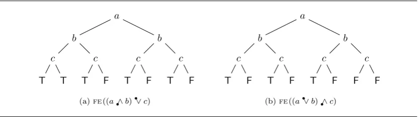
in T as evaluation trees, or simply trees for short. Figure 2.1 shows the trees corresponding to

the evaluations of (a ∨rb b) ∧_rb c and (a ∧_rb b) ∨rb c.

Returning to our example, we have seen that the tree corresponding to the evaluation of

(a ∨rb b) ∧_rb c can be composed from the tree corresponding to the evaluation of a ∨rb b and that

corresponding to the evaluation of c. We said above that if a ∨rb b yieldedT, we would proceed

with the evaluation of c. This can be seen as replacing each T-leaf in the tree corresponding

to the evaluation of a ∨rb b with the tree that corresponds to the evaluation of c. Formally

we define the leaf replacement operator, ‘replacement’ for short, on trees inT as follows. Let

X, X0, X00, Y, Z ∈ T and a ∈ A. The replacement of T with Y and F with Z in X, denoted X[T7→Y,F7→Z], is defined recursively as

T[T7→Y,F7→Z] =Y

F[T7→Y,F7→Z] =Z

(X0_Ea_DX00)[T7→Y,F7→Z] =X0[T7→Y,F7→Z]_Ea_DX00[T7→Y,F7→Z].

We note that the order in which the replacements of the leaves ofX is listed inside the brackets

is irrelevant. We will adopt the convention of not listing any identities inside the brackets, i.e.,

X[F7→Y] =X[T7→T,F7→Y].

Furthermore we let replacements associate to the left. We also use that fact that

X[T7→Y][F7→Z] =X[T7→Y,F7→Z]

ifY does not containF, which can be shown by a trivial induction. Similarly,

X[F7→Z][T7→Y] =X[T7→Y,F7→Z]

if Z does not contain T. We now have the terminology and notation to formally define the

evaluation of FEL-terms.

Definition 2.2. Let Abe a countable set of atoms and let T be the set of all finite binary trees overAwith leaves in {T,F}. We define the unaryFull Evaluationfunction fe : FT→ T as:

fe(T) =T fe(F) =F

fe(a) =TEaDF fora∈A

fe(¬P) =fe(P)[T7→F,F7→T]

fe(P ∧rb Q) =fe(P)[T7→fe(Q),F7→fe(Q)[T7→F]]

fe(P ∨rb Q) =fe(P)[T7→fe(Q)[F7→T],F7→fe(Q)].

Note that because we require A to be a set, T is also a set. By a trivial induction we can

show that all trees in the image of_fe are perfect binary trees, i.e., all their paths are of equal

length. As we can see from the definition on atoms, the evaluation continues in the left branch

if an atom yields T and in the right branch if it yields F. Revisiting our example once more,

we indeed see how the evaluation of a ∨rb b is composed of the evaluation of a followed by the

evaluation ofb in case ayields Fand by the evaluation ofb, but with a constant yield of T, in

caseayieldsT. We can compute_fe(a ∨rb b) as follows.

fe(a ∨rb b) = (TEaDF)[T7→(TEbDF)[F7→T],F7→(TEbDF)]

= (T_Ea_DF)[T7→(T_Eb_DT),F7→(T_Eb_DF)]

Now the evaluation of (a ∨rb b) ∧_rb cis a composition of this tree and T_Ec_DF, as can be seen in Figure 2.1b. a b c T T c T F b c T F c T F

(a)fe((a ∧qa b)∨qa c)

a b c T F c T F b c T F c F F

(b)fe((a∨qa b) ∧qa c)

Figure 2.1: Trees depicting the evaluation of two FEL-terms. The evaluation starts at the

root. When (the atom at) an inner node yieldsTthe evaluation continues in its left branch

and when it yields Fit continues in its right branch. The leaves indicate the yield of the

terms as a whole.

Informally we see that two FEL-terms are equal when they not only yield the same truth

value given the truth values of their constituent atoms, but also contain the same atomsin the

same order. Consider for example the terms aand a ∧_rb (b ∨rb T) and note that the truth value

of both is determined entirely by the truth value ofa. Also note that since b occurs aftera in

the second term, no side effect ofbcould ever affecta. When both terms would be placed in the

context of another term, e.g., a ∧_rb cand (a ∧_rb (b ∨rb T)) ∧_rb c, the situation changes. A side effect

of bmight, for example, be that c will yieldF. In that case the truth value of the first term is

determined by aand c, while that of the second term is alwaysF. We are now ready to define

Fully Evaluated Left-Sequential Logic.

Definition 2.3. A Fully Evaluated Left-Sequential Logic (FEL) is a logic that satisfies the consequences of_fe-equality. Free Fully Evaluated Left-Sequential Logic (FFEL)is the fully evaluated left-sequential logic that satisfies no more consequences than those of_fe-equality, i.e., for all P, Q∈FT,

FELP =Q ⇐= _fe(P) =_fe(Q) and FFELP=Q ⇐⇒ _fe(P) =_fe(Q).

It is not considered standard to define a logic equationally, but in this case we feel it is warranted to avoid having to mix the connectives from PL with those from FEL.

There is an immediate correspondence between trees and sets of traces, namely the paths of such trees annotated with the truth value of each internal node. For example, Figure 2.1a would correspond to the set of traces

{(aTbTcT,T),(aTbTcF,T),(aTbFcT,T),(aTbFcF,F), (aFbTcT,T),(aFbTcF,F),(aFbFcT,T),(aFbFcF,F)}.

This means we could have defined the image offe to be sets of such annotated traces. We chose

to define FEL with tree semantics rather than with trace semantics because the former affords us a more succinct notation.

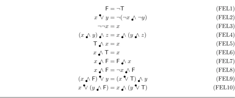
F=¬T (FEL1)

x ∨rb y=¬(¬x ∧_rb ¬y) (FEL2)

¬¬x=x (FEL3)

(x ∧_rb y) ∧_rb z=x ∧_rb (y ∧_rb z) (FEL4)

T ∧_rb x=x (FEL5)

x ∧_rb T=x (FEL6)

x ∧_rb F=F ∧_rb x (FEL7)

x ∧_rb F=¬x ∧_rb F (FEL8)

(x ∧_rb F) ∨rb y= (x ∨rb T) ∧_rb y (FEL9)

x ∨rb (y ∧_rb F) =x ∧_rb (y ∨rb T) (FEL10)

If two FEL-termssandt, possibly containing variables, are derivable by equational logic and

EqFFEL, we denote this by EqFFEL`s=tand say thatsandtare derivably equal. By virtue

of (FEL1) through (FEL3), ∧_rb is the dual of ∨rb and hence the duals of the equations in EqFFEL

are also derivable. We will use this fact implicitly throughout our proofs.

The following lemma shows some useful equations illustrating the special properties of terms

of the form x ∧_rb F and x ∨rb T. The first is an ‘extension’ of (FEL8) and the others show two

different ways how terms of the formx∨rb T, and by duality terms of the formx∧_rb F, can change

the main connective of a term.

Lemma 2.4. The following equations can all be derived by equational logic andEqFFEL.

1. x ∧_rb (y ∧_rb F) =¬x ∧_rb (y ∧_rb F) 2. (x ∨rb T) ∧_rb y=¬(x ∨rb T) ∨rb y

3. x ∨rb (y ∧_rb (z ∨rb T)) = (x ∨rb y) ∧_rb (z ∨rb T)

Proof. We derive the equations in order.

x ∧_rb (y ∧_rb F) = (x ∧_rb F) ∧_rb y by (FEL7) and (FEL4)

= (¬x ∧_rb F) ∧_rb y by (FEL8)

=¬x ∧_rb (y ∧_rb F) by (FEL7) and (FEL4)

(x ∨rb T) ∧_rb y= (x ∧_rb F) ∨rb y by (FEL9)

= (¬x ∧_rb F) ∨rb y by (FEL8)

= (¬x ∧_rb ¬T) ∨rb y by (FEL1)

=¬(x ∨rb T) ∨rb y by (FEL3) and (FEL2)

x ∨rb (y ∧_rb (z ∨rb T)) =x ∨rb (y ∨rb (z ∧_rb F)) by (FEL10)

= (x ∨rb y) ∨rb (z ∧_rb F) by the dual of (FEL4)

= (x ∨rb y) ∧_rb (z ∨rb T) by (FEL10)

Theorem 2.5. For all P, Q∈FT, ifEqFFEL`P =Q thenFFELP =Q.

Proof. It is immediately clear that identity, symmetry and transitivity are preserved. For

con-gruence we show only that for allP, Q, R∈FT, FFELP=Qimplies FFELR∧_rb P=R∧_rb Q.

The other cases proceed in a similar fashion. If FFELP =Q, then_fe(P) =_fe(Q) and hence

fe(P)[T7→F] =fe(Q)[T7→F], so

fe(R)[T7→fe(P),F7→fe(P)[T7→F]] =fe(R)[T7→fe(Q),F7→fe(Q)[T7→F]].

Therefore by definition of_fe, FFELR ∧_rb P=R ∧_rb Q.

The validity of the equations in EqFFEL is also easily verified. As an example we show this for (FEL8).

fe(P ∧rb F) =fe(P)[T7→F,F7→F[T7→F]] by definition

=_fe(P)[T7→F] because F[T7→F] =F

=_fe(P)[T7→F,F7→T][T7→F] by induction

=fe(¬P ∧_rb F),

2.1

FEL Normal Form

To aid in our completeness proof we define a normal form for FEL-terms. Due to the possible presence of side effects, FFEL does not identify terms which contain different atoms or the same atoms in a different order. Because of this, common normal forms for PL are not normal forms for FEL-terms. For example, rewriting a term to Conjunctive Normal Form or Disjunctive Normal Form may require duplicating some of the atoms in the term, thus yielding a term that is not derivably equal to the original. We first present the grammar for our normal form, before motivating it. The normal form we present here is an adaptation of a normal form proposed by Blok in [Blo11].

Definition 2.6. A term P ∈FTis said to be in FEL Normal Form (FNF)if it is generated by the following grammar.

P ∈FNF ::=PT | PF | PT ∧_rb P∗

P∗::=Pc | Pd Pc::=P` | P∗ ∧<sub>rb</sub> Pd Pd::=P` | P∗ ∨rb Pc P`::=a ∧_rb PT | ¬a ∧_rb PT PT::=T | a ∨rb PT PF::=F | a ∧_rb PF,

wherea∈A. We refer toP∗-forms as∗-terms, toP`<sub>-forms as`-terms, toP</sub>T_{-forms asT-terms}

and toPF_{-forms as F-terms. A term of the formP}T _{∧rb P}∗ _{is referred to as aT-∗-term.}

We immediately note that if it were not for the presence ofT andFwe could define a much

simpler normal form. In that case it would suffice to ‘push in’ or ‘push down’ the negations, thus

obtaining a Negation Normal Form, as exists for PL. Naturally if our setA of atoms is empty,

the truth value constants would be a normal form.

When considering the image of_fe we note that some trees only haveT-leaves, some only have

F-leaves and some have bothT-leaves andF-leaves. For any FEL-termP,_fe(P ∨rb T) is a tree

with onlyT-leaves, as can easily be seen from the definition of_fe. All termsP such that_fe(P)

only has T-leaves are rewritten to T-terms. Similarly _fe(P ∧_rb F) is a tree with only F-leaves.

All termsP such that_fe(P) only has F-leaves are rewritten to F-terms. The simplest trees in

the image of_fe that have bothT-leaves and F-leaves are_fe(a) fora∈A. Any (occurrence of

an) atom that determines (in whole or in part) the yield of a term, such asain this example, is

referred to as a determinative (occurrence of an) atom. This as opposed to a non-determinative

(occurrence of an) atom, such as theaina∨rb T, which does not determine (either in whole or in

part) the yield of the term. Note that a termP such thatfe(P) contains bothT and Fmust

contain at least one determinative atom.

Terms that contain at least one determinative atom will be rewritten to T-∗-terms. In T

-∗-terms we encode each determinative atom together with the non-determinative atoms that

occur between it and the next determinative atom in the term (reading from left to right) as an `-term. Observe that the first atom in an`-term is the (only) determinative atom in that`-term

and that determinative atoms only occur in `-terms. Also observe that the yield of an `-term

is the yield of its determinative atom. This is intuitively convincing, because the remainder of

the atoms in any`-term are non-determinative and hence do not contribute to its yield. The

T-term. A T-∗-term is the conjunction of a T-term encoding such atoms and a ∗-term, which

contains only conjunctions and disjunctions of`-terms. We could also have encoded such atoms

as an F-term and then taken the disjunction with a ∗-term to obtain a term with the same

semantics. We consider `-terms to be ‘basic’ in ∗-terms in the sense that they are the smallest

grammatical unit that influences the yield of the∗-term.

In the following,PT_{, P}`_{, etc. are used both to denote grammatical categories and as variables}

for terms in those categories. The remainder of this section is concerned with defining and

proving correct the normalization function f : FT → FNF. We will definef recursively using

the functions

fn: FNF→FNF and fc: FNF×FNF→FNF.

The first of these will be used to rewrite negated FNF-terms to FNF-terms and the second to rewrite the conjunction of two FNF-terms to an FNF-term. By (FEL2) we have no need for a dedicated function that rewrites the disjunction of two FNF-terms to an FNF-term.

We start by definingfn. Analyzing the semantics ofT-terms andF-terms together with the

definition offe on negations, it becomes clear thatfn must turnT-terms intoF-terms and vice

versa. We also remark thatfn must preserve the left-associativity of the∗-terms in T-∗-terms,

modulo the associativity within `-terms. We define fn _{: FNF → FNF as follows, using the}

auxiliary functionfn

1 :P∗→P∗to ‘push down’ or ‘push in’ the negation symbols when negating

a T-∗-term. We note that there is no ambiguity between the different grammatical categories

present in an FNF-term, i.e., any FNF-term is in exactly one of the grammatical categories identified in Definition 2.6.

fn(T) =F (2.1)

fn(a ∨rb PT) =a ∧_rb fn(PT) (2.2)

fn(F) =T (2.3)

fn(a ∧_rb PF) =a ∨rb fn(PF). (2.4)

fn(PT ∧_rb Q∗) =PT ∧_rb f₁n(Q∗) (2.5)

f₁n(a ∧_rb PT) =¬a ∧_rb PT (2.6)

f₁n(¬a ∧_rb PT) =a ∧_rb PT (2.7)

f1n(P∗ ∧rb Qd) =f1n(P∗) ∨ rb

f1n(Qd) (2.8)

f₁n(P∗ ∨rb Qc) =f₁n(P∗) ∧_rb f₁n(Qc) (2.9)

Now we turn to definingfc_{. These definitions have a great deal of inter-dependence so we first}

present the definition for fc _{when the first argument is a T-term. We see that the conjunction}

of a T-term with another term always yields a term of the same grammatical category as the

second conjunct.

fc(T, P) =P (2.10)

fc(a ∨rb PT, QT) =a ∨rb fc(PT, QT) (2.11)

fc(a ∨rb PT, QF) =a ∧_rb fc(PT, QF) (2.12)

fc(a ∨rb PT, QT ∧_rb R∗) =fc(a ∨rb PT, QT) ∧_rb R∗ (2.13)

For definingfc _{where the first argument is anF-term we make use of (FEL7) when dealing}

with conjunctions ofF-terms withT-∗-terms. The definition offc _{for the arguments used in the}

in these definitions, this does not create a circular definition. We also note that the conjunction

of anF-term with another term is always itself anF-term.

fc(F, PT) =fn(PT) (2.14)

fc(F, PF) =PF (2.15)

fc(F, PT ∧_rb Q∗) =fc(PT ∧_rb Q∗,F) (2.16)

fc(a ∧_rb PF, Q) =a ∧_rb fc(PF, Q) (2.17)

The case where the first conjunct is a T-∗-term is the most complicated. Therefore we first

consider the case where the second conjunct is aT-term. In this case we must make theT-term

part of the last (rightmost)`-term in theT-∗-term, so that the result will again be aT-∗-term.

For this ‘pushing in’ of the second conjunct we define an auxiliary functionfc

1 :P∗×PT→P∗.

fc(PT ∧_rb Q∗, RT) =PT ∧_rb f1c(Q∗, R T

) (2.18)

f₁c(a ∧_rb PT, QT) =a ∧_rb fc(PT, QT) (2.19)

f₁c(¬a ∧_rb PT, QT) =¬a ∧_rb fc(PT, QT) (2.20)

f₁c(P∗ ∧_rb Qd, RT) =P∗ ∧_rb f₁c(Qd, RT) (2.21)

f₁c(P∗ ∨rb Qc, RT) =P∗ ∨rb f₁c(Qc, RT) (2.22)

When the second conjunct is anF-term, the result will naturally be anF-term itself. So we

need to convert theT-∗-term to an F-term. Using (FEL4) we reduce this problem to converting

a∗-term to anF-term, for which we use the auxiliary functionf2c:P∗×PF→PF.

fc(PT ∧_rb Q∗, RF) =fc(PT, f₂c(Q∗, RF)) (2.23)

f2c(a ∧rb PT, RF) =a ∧rb fc(PT, RF) (2.24)

f₂c(¬a ∧_rb PT, RF) =a ∧_rb fc(PT, RF) (2.25)

f₂c(P∗ ∧_rb Qd, RF) =f₂c(P∗, f₂c(Qd, RF)) (2.26)

f₂c(P∗ ∨rb Qc, RF) =f₂c(P∗, f₂c(Qc, RF)) (2.27)

Finally we are left with conjunctions and disjunctions of twoT-∗-terms, thus completing the

definition offc_{. We use the auxiliary functionf}c

3 :P∗×PT∧rb P∗→P∗to ensure that the result

is aT-∗-term.

fc(PT ∧_rb Q∗, RT ∧_rb S∗) =PT ∧_rb f₃c(Q∗, RT ∧_rb S∗) (2.28)

f₃c(P∗, QT ∧_rb R`) =f<sub>1</sub>c(P∗, QT) ∧<sub>rb</sub> R` (2.29)

f3c(P∗, QT ∧rb (R∗ ∧rb Sd)) =f3c(P∗, QT ∧rb R∗) ∧rb Sd (2.30)

f₃c(P∗, QT ∧_rb (R∗ ∨rb Sc)) =f₁c(P∗, QT) ∧_rb (R∗ ∨rb Sc) (2.31)

As promised, we now define the normalization functionf : FT→FNF recursively, usingfn

andfc_{, as follows.}

f(a) =T ∧_rb (a ∧_rb T) (2.32)

f(T) =T (2.33)

f(F) =F (2.34)

f(¬P) =fn(f(P)) (2.35)

f(P ∧_rb Q) =fc(f(P), f(Q)) (2.36)

Theorem 2.7. For any P ∈FT,f(P)terminates,f(P)∈FNFandEqFFEL`f(P) =P.

In Appendix A.1 we first prove a number of lemmas showing that the definitionsfn _andfc

are correct and use those to prove the theorem. The reader might wonder why we have used a normalization function rather than a term rewriting system to prove the correctness of FNF. The main reason is the author’s lack of experience with term rewriting systems, although the fact that using a function relieves us of the need to prove the confluence of the induced rewriting system, thus simplifying the proof, is also a factor.

2.2

Tree Structure

In Section 2.3 we will prove that EqFFEL axiomatizes FFEL by showing that for P ∈ FNF

we can invert _fe(P). To do this we need to prove several structural properties of the trees in

the image of _fe. In the definition of_fe we can see how_fe(P ∧_rb Q) is assembled from_fe(P)

and _fe(Q) and similarly for _fe(P ∨rb Q). To decompose these trees we will introduce some

notation. The trees in the image of _fe are all finite binary trees over Awith leaves in {T,F},

i.e., _fe[FT]⊆ T. We will now also consider the set T of binary trees over A with leaves in

{T,F,}, where the ‘’ symbol is pronounced ‘box’. Similarly we considerT1,2, the set of binary

trees overAwith leaves in{T,F,1,2}. The,1 and2 will be used as placeholders when

composing or decomposing trees. Replacement of the leaves of trees in T and T1,2 by trees

(either in T, T orT1,2) is defined analogous to replacement for trees inT, adopting the same

notational conventions.

For example we have by definition offe that fe(P ∧_rb Q) can be decomposed as

fe(P)[T7→1,F7→2][17→fe(Q),27→fe(Q)[T7→F]],

where fe(P)[T7→ 1,F7→ 2] ∈ T1,2 and fe(Q) and fe(Q)[T 7→ F] are in T. We note that

this only works because the trees in the image offe, or more general, inT, do not contain any

boxes. Similarly, as we discussed previously,_fe(P ∧_rb F) =_fe(P)[T7→F], which we can write as

fe(P)[T7→][7→F]. We start by analyzing thefe-image of`-terms.

Lemma 2.8 (Structure of`-terms). There is no`-termP such that _fe(P) can be decomposed as X[ 7→ Y] with X ∈ T and Y ∈ T, where X 6=, but does contain , and Y contains occurrences of both TandF.

Proof. Let P be some `-term. When we analyze the grammar of P we find that one branch

from the root of_fe(P) will only containTand notFand the other branch vice versa. Hence if

fe(P) =X[7→Y] andY contains occurrences of bothTandF, thenY must contain the root

and henceX=.

By definition a ∗-term contains at least one `-term and hence for any ∗-term P, _fe(P)

contains both TandF. The following lemma provides the_fe-image of the rightmost`-term in

a ∗-term to witness this fact.

Lemma 2.9 (Determinativeness). For all ∗-terms P,_fe(P)can be decomposed as X[7→Y] with X∈ T andY ∈ T such that X containsandY =_fe(Q) for some`-termQ. Note that X may be . We will refer to Y as the witness for this lemma for P.

Proof. By induction on the complexity of∗-termsP modulo the complexity of`-terms. In the

base case P is an `-term and _fe(P) =[7→_fe(P)] is the desired decomposition by Lemma

We treat only the case for _fe(P ∧_rb Q), the case for _fe(P ∨rb Q) is analogous. LetX[7→Y]

be the decomposition for_fe(Q) which we have by induction hypothesis. Since by definition of

fe on ∧rb we have

fe(P ∧rb Q) =fe(P)[T7→fe(Q),F7→fe(Q)[T7→F]], we also have

fe(P ∧rb Q) =fe(P)[T7→X[7→Y],F7→fe(Q)[T7→F]]

=_fe(P)[T7→X,F7→_fe(Q)[T7→F]][7→Y],

where the second equality is due to the fact that the only boxes in

fe(P)[T7→X,F7→fe(Q)[T7→F]]

are those occurring inX. This gives our desired decomposition.

The following lemma illustrates another structural property of trees in the image of ∗-terms

under_fe, namely that the left branch of any determinative atom in such a tree is different from

its right branch.

Lemma 2.10(Non-decomposition). There is no∗-termP such that _fe(P) can be decomposed asX[7→Y] withX ∈ T andY ∈ T, whereX 6=andX contains , but not Tor F. Proof. By induction onP modulo the complexity of`-terms. The base case covers`-terms and

follows immediately from Lemma 2.9 (_fe(P) contains occurrences of bothTandF) and Lemma

2.8 (no non-trivial decomposition exists that contains both). For the induction we assume that

the lemma holds for all∗-terms with lesser complexity thanP ∧_rb Qand P ∨rb Q.

We start with the case for_fe(P∧_rb Q). Suppose for contradiction that_fe(P∧_rb Q) =X[7→Y]

withX6=andX not containing any occurrences ofTorF. LetR be a witness of Lemma 2.9

forP. Now note that _fe(P ∧_rb Q) has a subtree

R[T7→fe(Q),F7→fe(Q)[T7→F]].

BecauseY must contain both the occurrences ofFin the one branch from the root of this subtree

as well as the occurrences offe(Q) in the other (because they contain T and F), Lemma 2.8

implies thatY must (strictly) contain fe(Q) and fe(Q)[T7→F]. Hence there is aZ ∈ T such

that fe(P) = X[ 7→ Z], which violates the induction hypothesis. The case for fe(P ∨rb Q)

proceeds analogously.

We now arrive at two crucial definitions for our completeness proof. When considering∗-terms

we already know that_fe(P ∧_rb Q) can be decomposed as

fe(P)[T7→1,F7→2][17→fe(Q),27→fe(Q)[T7→F]].

Our goal now is to give a definition for a type of decomposition so that this is the only such

decomposition forfe(P ∧_rb Q). We also ensure thatfe(P ∨rb Q) does not have a decomposition of

that type, so that we can distinguishfe(P ∧_rb Q) fromfe(P ∨rb Q). Similarly, we define another

type of decomposition so thatfe(P ∨rb Q) can only be decomposed as

fe(P)[T7→1,F7→2][17→fe(Q)[F7→T],27→fe(Q)]

Definition 2.11. The pair (Y, Z) ∈ T1,2× T is a candidate conjunction decomposition

(ccd) ofX ∈ T, if

• X=Y[17→Z,27→Z[T7→F]],

• Y contains both1 and2,

• Y contains neitherT norF, and

• Z contains bothT andF.

Similarly, (Y, Z)is acandidate disjunction decomposition (cdd)of X, if

• X=Y[17→Z[F7→T],27→Z],

• Y contains both1 and2,

• Y contains neitherT norF, and

• Z contains bothT andF.

The ccd and cdd are not necessarily the decompositions we are looking for, because, for

example, _fe((P ∧_rb Q) ∧_rb R) has a ccd (_fe(P)[T 7→ 1,F 7→ 2],fe(Q ∧rb R)), whereas the

decomposition we need is (_fe(P ∧_rb Q)[T 7→ 1,F 7→ 2],fe(R)). Therefore we refine these

definitions to obtain the decompositions we seek.

Definition 2.12. The pair(Y, Z)∈ T1,2× T is aconjunction decomposition (cd)ofX ∈ T,

if it is a ccd of X and there is no other ccd(Y0, Z0) ofX where the depth ofZ0 is smaller than that of Z. Similarly, (Y, Z) is a disjunction decomposition (dd) of X, if it is a cdd of X and there is no other cdd(Y0, Z0) ofX where the depth of Z0 is smaller than that ofZ.

Theorem 2.13. For any ∗-term P ∧_rb Q, i.e., with P ∈P∗ and Q∈ Pd_,

fe(P ∧rb Q) has the (unique) cd

(_fe(P)[T7→1,F7→2],fe(Q))

and no dd. For any∗-termP ∨rb Q, i.e., with P∈P∗ andQ∈Pc,fe(P ∨rb Q)has no cd and its (unique) dd is

(_fe(P)[T7→1,F7→2],fe(Q)).

Proof. We first treat the case for P ∧_rb Q and start with cd. Note that fe(P ∧_rb Q) has a ccd

(fe(P)[T7→1,F7→2],fe(Q)) by definition offe (for the first condition) and by Lemma 2.9

(for the fourth condition). It is immediate that it satisfies the second and third conditions. It also

follows that for any ccd (Y, Z) eitherZcontains or is contained infe(Q), for suppose otherwise,

thenY will contain an occurrence ofTor ofF, namely those we know by Lemma 2.9 that_fe(Q)

has. Therefore it suffices to show that there is no ccd (Y, Z) where Z is strictly contained in

fe(Q). Suppose for contradiction that (Y, Z) is such a ccd. IfZ is strictly contained in fe(Q)

we can decompose_fe(Q) as_fe(Q) =U[7→Z] for someU ∈ Tthat contains but is not equal

to. By Lemma 2.10 this implies thatU containsTorF. But then so doesY, because

Y =_fe(P)[T7→U[7→1],F7→U[7→2]],

and so (Y, Z) is not a ccd forfe(P ∧_rb Q). Therefore (fe(P)[T7→ 1,F7→2],fe(Q)) is the

unique cd for_fe(P ∧_rb Q).

Now for the dd. It suffices to show that there is no cdd for _fe(P ∧_rb Q). Suppose for

contradiction that (Y, Z) is a cdd for_fe(P ∧_rb Q). We note thatZ cannot be contained in_fe(Q),

for then by Lemma 2.10 Y would contain T or F. So Z (strictly) contains _fe(Q). But then

because

we would have by Lemma 2.9 that_fe(P ∧_rb Q) does not contain an occurrence of_fe(Q)[T7→F].

But the cd of _fe(P ∧_rb Q) tells us that it does, contradiction! Therefore there is no cdd, and

hence no dd, for_fe(P ∧_rb Q). The case for_fe(P ∨rb Q) proceeds analogously.

At this point we have the tools necessary to invert_fe on∗-terms, at least down to the level

of`-terms. We note that we can easily detect if a tree in the image of<sub>fe</sub> is in the image ofP`_,

because all leaves to the left of the root are one truth value, while all the leaves to the right are

the other. To invert_fe onT-∗-terms we still need to be able to reconstruct_fe(PT_{) and}

fe(Q∗)

from_fe(PT _{∧rb Q}∗_{). To this end we define aT-∗-decomposition.}

Definition 2.14. The pair (Y, Z) ∈ T × T is a T-∗-decomposition (tsd) of X ∈ T, if X=Y[7→Z],Y does not containT orFand there is no decomposition (U, V)∈ T× T ofZ such that

• Z =U[7→V],

• U contains,

• U 6=, and

• U contains neitherT nor F.

Theorem 2.15. For any T-termP and∗-termQthe (unique) tsd of fe(P ∧_rb Q)is

(fe(P)[T7→],fe(Q)).

Proof. First we observe that (_fe(P)[T7→],_fe(Q)) is a tsd because by definition of_fe on ∧_rb

we have_fe(P)[T7→_fe(Q)] =_fe(P ∧_rb Q) and_fe(Q) is non-decomposable by Lemma 2.10.

Suppose for contradiction that there is another tsd (Y, Z) of_fe(P ∧_rb Q). NowZ must contain

or be contained in_fe(Q) for otherwise Y would contain T orF, i.e., the ones we know_fe(Q)

has by Lemma 2.9.

If Z is strictly contained in_fe(Q), then_fe(Q) = U[7→Z] for some U ∈ T with U 6=

andU not containingTorF(because thenY would too). But this violates Lemma 2.10, which

states that no such decomposition exists. IfZ strictly contains_fe(Q), thenZ contains at least

one atom from P. But the left branch of any atom in _fe(P) is equal to its right branch and

henceZ is decomposable. Therefore (fe(P)[T7→],fe(Q)) is theuniquetsd offe(P ∧_rb Q).

2.3

Completeness

With the two theorems from the previous section, we can prove completeness for FFEL. We define

three auxiliary functions to aid in our definition of the inverse of_feon FNF. Let cd :T → T1,2×T

be the function that returns the conjunction decomposition of its argument, dd of the same type

its disjunction decomposition and tsd :T → T× T its T-∗-decomposition. Naturally, these

functions are undefined when their argument does not have a decomposition of the specified type.

Each of these functions returns a pair and we will use cd1(dd1, tsd1) to denote the first element

of this pair and cd2(dd2, tsd2) to denote the second element.

We define g :T →FT using the functions gT: T →FT for inverting trees in the image of

T-terms andgF,g`and g∗ of the same type for inverting trees in the image ofF-terms,`-terms

and∗-terms, respectively. These functions are defined as follows.

gT(X) = (

T ifX=T

We note that we might as well have used the right branch from the root in the recursive case. We chose the left branch here to more closely mirror the definition of the corresponding function

for FSCL_se, defined in Chapter 3.

gF(X) =

(

F ifX =F

a ∧_rb gF(Z) ifX =Y _Ea_DZ (2.39)

Similarly, we could have taken the left branch in this case.

g`(X) =

        

a ∧_rb gT_{(Y) ifX =Y}

Ea_DZ for somea∈A

andY only hasT-leaves

¬a ∧_rb gT_{(Z) ifX =Y}

Ea_DZ for somea∈A

andZ only hasT-leaves

(2.40)

g∗(X) =

  

 

g∗(cd1(X)[17→T,27→F]) ∧rb g∗(cd2(X)) ifX has a cd

g∗(dd1(X)[17→T,27→F]) ∨rb g∗(dd2(X)) ifX has a dd

g`_{(X) otherwise}

(2.41)

We can immediately see how Theorem 2.13 will be used in the correctness proof ofg∗.

g(X) =     

gT_{(X) ifX has only T-leaves}

gF(X) ifX has only F-leaves

gT_(tsd

1(X)[7→T]) ∧rb g∗(tsd2(X)) otherwise

(2.42)

Similarly, we can see how Theorem 2.15 is used in the correctness proof ofg. It should come as

no surprise thatg is indeed correct and inverts_fe on FNF.

Theorem 2.16. For allP ∈FNF,g(_fe(P))≡P.

The proof for this theorem can be found in Appendix A.2. For the sake of completeness, we separately state the completeness result below.

Theorem 2.17. For allP, Q∈FT, if FFELP =QthenEqFFEL`P =Q.

Proof. It suffices to show that for P, Q ∈ FNF, fe(P) = fe(Q) implies P ≡ Q. To see this

suppose thatP0 andQ0are two FEL-terms andfe(P0) =fe(Q0). We know thatP0 is derivably

equal to an FNF-termP, i.e., EqFFEL`P0=P, and thatQ0 is derivably equal to an FNF-term

Q, i.e., EqFFEL`Q0 =Q. Theorem 2.5 then gives usfe(P0) =fe(P) and fe(Q0) =fe(Q).

Hence by the result P ≡ Q and in particular EqFFEL ` P = Q. Transitivity then gives us

EqFFEL`P0 =Q0 as desired.

CHAPTER 3

Free Short-Circuit Logic (FSCL)

In this chapter we define Free Short-Circuit Logic on evaluation trees and present the set of equations EqFSCL, which we will prove axiomatizes this logic in Section 2.3. Formally, SCL-terms are built up from atomic propositions that may have side effects, called atoms, the truth

value constantsTfor true andFfor false and the connectives¬for negation, ∧_rb for (short-circuit)

left-sequential conjunction and ∨rb for (short-circuit) left-sequential disjunction.

Definition 3.1. LetAbe a countable set of atoms. SCL-terms (ST)have the following gram-mar presented in Backus-Naur Form.

P ∈ST ::=a∈A | T | F | ¬P | (P ∧_rb P) | (P ∨rb P)

As is the case with FEL, ifA=∅then resulting logic is trivial.

First we return for a moment to our motivation for left-sequential logics, i.e., propositional

terms as used in programming languages. We will consider the SCL-term a ∨rb band informally

describe its evaluation, naturally using a short-circuit evaluation strategy. We start by evaluating

a and let its yield determine our next action. If a yielded F we proceed by evaluating b, i.e.,

the yield of the term as a whole will be the yield of b. If ayielded T, we already know at this

point that a ∨rb b will yieldT. We skip the evaluation of b and let the term yield T, i.e., b is

short-circuited.

Considering the more complex term (a ∨rb b) ∧_rb c, we find that we start by evaluatinga ∨rb b

and if it yields Twe proceed by evaluatingc. If it yieldsFwe skip the evaluation ofc, because

we know the term will yieldF. This example shows that evaluating SCL-terms is an interactive

procedure, where the yield of the previous atom is needed to determine which atom to evaluate next. We believe these semantics are best captured in trees. Hence we will define equality of

SCL-terms using (evaluation) trees. We define the setT of finite binary trees overAwith leaves

in {T,F} recursively. We have that

T∈ T, F∈ T, and (X _Ea_DY)∈ T for anyX, Y ∈ T anda∈A.

In the expression X _E a _D Y the root is represented by a, the left branch by X and the

right branch by Y. We define the depth of a tree X recursively by d(T) = d(F) = 0 and

d(Y _Ea_DZ) = 1 + max(d(Y), d(Z)) fora∈A. The reason for our choice of notation for trees

will become apparent in Chapter 4. We refer to trees inT as evaluation trees, or trees for short.

Returning to our example, we have seen that the tree corresponding to the evaluation of

(a ∨rb b) ∧_rb c can be composed from the tree corresponding to the evaluation of a ∨rb b and that

corresponding to the evaluation of c. We said above that if a ∨rb b yieldedT, we would proceed

with the evaluation of c. This can be seen as replacing each T-leaf in the tree corresponding

to the evaluation of a ∨rb b with the tree that corresponds to the evaluation of c. Formally

we define the leaf replacement operator, ‘replacement’ for short, on trees inT as follows. Let

X, X0, X00Y, Z ∈ T and a ∈ A. The replacement of T with Y and F with Z in X, denoted X[T7→Y,F7→Z], is defined recursively as

T[T7→Y,F7→Z] =Y

F[T7→Y,F7→Z] =Z

(X0_Ea_DX00)[T7→Y,F7→Z] =X0[T7→Y,F7→Z]_Ea_DX00[T7→Y,F7→Z].

We note that the order in which the replacements of the leaves ofX is listed inside the brackets

is irrelevant. We will adopt the convention of not listing any identities inside the brackets, i.e.,

X[F7→Y] =X[T7→T,F7→Y].

Furthermore we let replacements associate to the left. We also use that fact that

X[T7→Y][F7→Z] =X[T7→Y,F7→Z]

ifY does not containF, which can be shown by a trivial induction. Similarly,

X[F7→Z][T7→Y] =X[T7→Y,F7→Z]

if Z does not contain T. We now have the terminology and notation to formally define the

mapping from SCL-terms to evaluation trees.

Definition 3.2. LetAbe a countable set of atoms and letT be the set all finite binary trees over Awith leaves in{T,F}. We define the unaryShort-Circuit Evaluationfunctionse : ST→ T

as:

se(T) =T se(F) =F

se(a) =TEaDF fora∈A

se(¬P) =se(P)[T7→F,F7→T] se(P ∧rb Q) =se(P)[T7→se(Q)]

se(P ∨rb Q) =se(P)[F7→se(Q)].

As we can see from the definition on atoms, the evaluation continues in the left branch if an

atom yieldsTand in the right branch if it yieldsF. Revisiting our example once more, we indeed

see how the evaluation ofa ∨rb bis composed of the evaluation ofafollowed by the evaluation of

bin caseayieldsF. We can compute

se(a ∨rb b) = (TEaDF)[F7→(TEbDF)]

=T_Ea_D(T_Eb_DF).

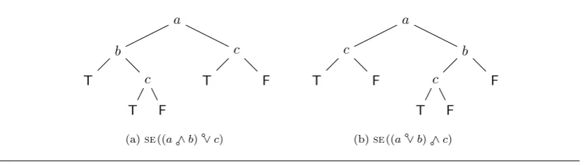
Now the evaluation of (a ∨rb b) ∧_rb cis a composition of this tree andT_Ec_DF, as can be seen in

a

b

T c

T F

c

T F

(a)se((a∧qa b) ∨qa c)

a

c

T F

b

c

T F F

(b)se((a∨qa b) ∧qa c)

Figure 3.1: Trees depicting the evaluation of two SCL-terms. The evaluation starts at the

root. When (the atom at) an inner node yieldsTthe evaluation continues in its left branch

and when it yields Fit continues in its right branch. The leaves indicate the yield of the

terms as a whole.

These trees show us that a function of the yield of the atoms in an SCL-term is insufficient to determine the semantics of the term as a whole. They show us that we must also consider the

(conditional) order in which the atoms occur in the term. In particular we see that inP ∨rb Q,Q

will be short-circuited ifP yieldsT, while inP ∧_rb Q, it will be short-circuited if P yieldsF. We

are now ready to define Short-Circuit Logic on evaluation trees.

Definition 3.3. Free Short-Circuit Logic (FSCL_se) is the logic that satisfies exactly the consequences of _se-equality, i.e., for all P, Q∈ST,

FSCL_se P =Q ⇐⇒ _se(P) =_se(Q).

Using the completeness result we shall prove in Section 3.3, we will show that FSCL_se is in

fact equivalent to FSCL as defined by Bergstra and Ponse in [BP10b]. This should come as no surprise given the tree-like structure that Proposition Algebra terms exhibit, see, e.g., [BP11] or [BP12].

We choose a representation ofT as trees rather than as sets of traces, i.e., the paths of those

trees annotated with truth values for the atoms, because the tree notation allows us to be more succinct. These tree semantics were first given, although presented as trace semantics, by Ponse in [Pon11].

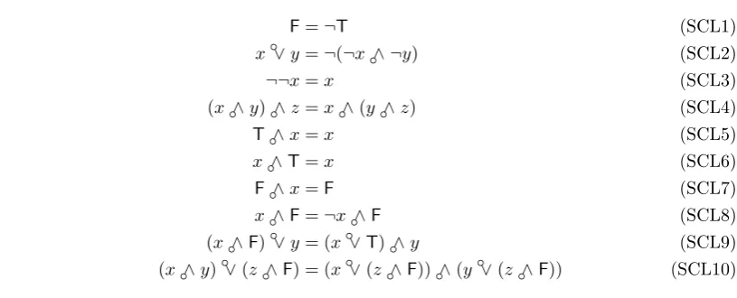
We now turn to the set of equations EqFSCL, listed in Table 3.1, which we will show in

Section 3.3 is an axiomatization of FSCL_se. This set of equations is based on one presented by

Bergstra and Ponse in [BP10b]. If two SCL-termssandt, where we extend the definition to allow

for terms containing variables, are derivable by equational logic and EqFSCL, we denote this by

EqFSCL`s=tand say thatsandtare derivably equal. As a consequence of (SCL1) through

(SCL3), ∧_rb is the dual of ∨rb and hence the duals of the equations in EqFSCL are also derivable.

We will use this fact implicitly throughout our proofs. Observe that unlike with EqFFEL, we have an equation in EqFSCL for (a special case of) distributivity, i.e., (SCL10).

The following lemma shows some equations that will prove useful in Section 3.1. These

equations show how terms of the formx∧_rb Fandx∨rb Tcan be used to change the order in which

F=¬T (SCL1)

x ∨rb y=¬(¬x ∧_rb ¬y) (SCL2)

¬¬x=x (SCL3)

(x ∧_rb y) ∧_rb z=x ∧_rb (y ∧_rb z) (SCL4)

T ∧_rb x=x (SCL5)

x ∧_rb T=x (SCL6)

F ∧_rb x=F (SCL7)

x ∧_rb F=¬x ∧_rb F (SCL8)

(x ∧_rb F) ∨rb y= (x ∨rb T) ∧_rb y (SCL9)

(x _b∧_r y) ∨rb (z ∧_rb F) = (x ∨rb (z _b∧_r F)) ∧_rb (y br∨(z ∧_rb F)) (SCL10)

Lemma 3.4. The following equations can all be derived by equational logic andEqFSCL.

1. (x ∨rb y) ∧_rb (z ∧_rb F) = (¬x ∨br (z ∧_rb F)) ∧_rb (y ∧_rb (z ∧_rb F)) 2. (x ∨rb (y ∧_rb F)) ∧_rb (z ∧_rb F) = (¬x ∨rb (z ∧_rb F)) ∧_rb (y ∧_rb F) 3. (x ∧_rb (y ∨rb T)) ∨rb (z ∧_rb F) = (x ∨br (z ∧_rb F)) _b∧_r (y ∨rb T) Proof. We derive the equations in order.

(x ∨rb y) ∧_rb (z ∧_rb F)

= (x ∨rb y) ∧_rb ((z ∧_rb F) ∧_rb F) by (SCL7) and (SCL4)

= (x ∨rb y) ∧_rb (¬(z ∧_rb F) ∧_rb F) by (SCL8)

= ((x ∨rb y) ∧_rb ¬(z ∧_rb F)) ∧_rb F by (SCL4)

= ((¬x ∧_rb ¬y) ∨rb (z ∧_rb F)) ∧_rb F by (SCL8), (SCL2) and (SCL3)

= ((¬x ∨rb (z ∧_rb F)) ∧_rb (¬y ∨rb (z ∧_rb F))) ∧_rb F by (SCL10)

= (¬x ∨rb (z ∧_rb F)) ∧_rb ((¬y ∨rb (z ∧_rb F)) ∧_rb F) by (SCL4)

= (¬x ∨rb (z ∧_br F)) ∧_rb ((y _b∧_r ¬(z ∧_rb F)) ∧_rb F) by (SCL8), (SCL2) and (SCL3)

= ((¬x ∨rb (z ∧_br F)) ∧_rb y) _b∧_r (¬(z ∧_rb F) ∧_rb F) by (SCL4)

= ((¬x ∨rb (z ∧_rb F)) ∧_rb y) ∧_rb ((z ∧_rb F) ∧_rb F) by (SCL8)

= ((¬x ∨rb (z ∧_rb F)) _br∧y) ∧_rb (z ∧_rb F) by (SCL4) and (SCL7)

= (¬x ∨rb (z ∧_rb F)) _br∧(y ∧_rb (z ∧_rb F)) by (SCL4)

(x ∨rb (y ∧_rb F)) ∧_rb (z ∧_rb F)

= (¬x ∨rb (z ∧_rb F)) ∧_rb ((y ∧_rb F) ∧_rb (z ∧_rb F)) by part (1) of this lemma

= (¬x ∨rb (z ∧_rb F)) ∧_rb (y ∧_rb F) by (SCL7) and (SCL4)

(x ∧_rb (y ∨rb T)) ∨rb (z ∧_rb F)

= (x ∨rb (z ∧_rb F)) ∧_rb ((y b∨r T) ∨rb (z ∧_rb F)) by (SCL10)

= (x ∨rb (z ∧_rb F)) _b∧_r (y ∨rb T) by the duals of (SCL7) and (SCL4)

Theorem 3.5. For all P, Q∈ST, if EqFSCL`P=Qthen FSCL_se P =Q.

Proof. To see that identity, symmetry, transitivity and congruence hold in FSCL_se, we refer the

reader to the proof of Theorem 2.5 and note that the proofs for FSCL_se are highly similar.

Verifying the validity of the equations in EqFSCL is cumbersome, but not difficult. As an example we show it for (SCL3). We have

se(¬¬P) =se(P)[T7→F,F7→T][T7→F,F7→T] =se(P) by a trivial structural induction on evaluation trees.

3.1

SCL Normal Form

To aid in our completeness proof we define a normal form for SCL-terms. Because the atoms in SCL-terms may have side effects common normal forms for PL such as Conjunctive Normal Form

or Disjunctive Normal Form are not normal forms for SCL. For example, the terma ∧_rb (b ∨rb c)

shows that the evaluation trees of these terms are not the same. Our normal form is inspired by the FEL Normal Form presented in Chapter 2. We present the grammar for our normal form before we motivate it.

Definition 3.6. A termP∈STis said to be inSCL Normal Form (SNF)if it is generated by the following grammar.

P ∈SNF ::=PT | PF | PT ∧_rb P∗

P∗::=Pc | Pd Pc::=P` | P∗ ∧<sub>rb</sub> Pd Pd::=P` | P∗ ∨rb Pc

P`::= (a ∧_rb PT) ∨rb PF | (¬a ∧_rb PT) ∨rb PF PT::=T | (a _br∧PT) ∨rb PT

PF::=F | (a ∨rb PF) ∧_rb PF,

wherea∈A. We refer toP∗-forms as∗-terms, toP`-forms as`-terms, toPT-forms asT-terms and toPF-forms as F-terms. A term of the formPT ∧_rb P∗ is referred to as aT-∗-term.

Without the presence ofTandFin our language, a traditional Negation Normal Form would

have sufficed. Furthermore, ifA=∅, an even more trivial normal form could be used, i.e., just

TorF.

When considering trees in the image ofse we note that some trees only haveT-leaves, some

onlyF-leaves and some both T-leaves and F-leaves. For any SCL-term P,se(P ∨rb T) is a tree

with onlyT-leaves, as can easily be seen from the definition ofse. All termsP such thatse(P)

is a tree with onlyT-leaves are rewritten to T-terms. Similarly, for any term P, _se(P ∧_rb F) is

a tree with only F-leaves. All P such that _se(P) has only F-leaves are rewritten to F-terms.

The simplest trees in the image of_se that have both types of leaves are_se(a) fora∈A. Any

(occurrence of an) atom that determines (in whole or in part) the yield of the term, such asa

in this example, is referred to as a determinative (occurrence of an) atom. This as opposed to

a non-determinative (occurrence of an) atom, such as theain a ∨rb T, which does not determine

(either in whole or in part) the yield of the term. Note that a termP such that_se(P) contains

bothTandFmust contain at least one determinative atom.

Terms that contain at least one determinative atom will be rewritten to T-∗-terms. In T

-∗-terms we encode each determinative atom together with the non-determinative atoms that

occur between it and the next determinative atom in the term (reading from left to right) as an `-term. Observe that the first atom in an`-term is the (only) determinative atom in that`-term

and that determinative atoms only occur in `-terms. Also observe that the yield of an `-term

is the yield of its determinative atom. This is intuitively convincing, because the remainder of

the atoms in any`-term are non-determinative and hence do not contribute to its yield. The

non-determinative atoms that may occur before the first determinative atom are encoded as a

T-term. A T-∗-term is the conjunction of a T-term encoding such atoms and a ∗-term, which

contains only conjunctions and disjunctions of`-terms. We could also have encoded such atoms

as an F-term and then taken the disjunction with a ∗-term to obtain a term with the same

semantics. We consider `-terms to be ‘basic’ in∗-terms in the sense that they are the smallest

grammatical unit that influences the yield of the∗-term.

The `-terms in SNF are more complex than those in FEL Normal Form, because short-circuiting allows for the possibility of evaluating different non-determinative atoms depending on

are more complex. Although the atoms occurring in them are not determinative, their yield can

influence which atoms in theT-term (F-term) are evaluated next.

We use PT_{, P}∗_{, etc. both to denote grammatical categories and as variables for terms in}

those categories. The remainder of this section is concerned with defining and proving correct

the normalization functionf : ST→SNF. We will definef recursively using the functions

fn: SNF→SNF and fc: SNF×SNF→SNF.

The first of these will be used to rewrite negated SNF-terms to SNF-terms and the second to rewrite the conjunction of two SNF-terms to an SNF-term. By (SCL2) we have no need for a dedicated function that rewrites the disjunction of two SNF-terms to an SNF-term.

We start by definingfn. Analyzing the semantics ofT-terms andF-terms together with the

definition ofse on negations, it becomes clear thatfn must turnT-terms intoF-terms and vice

versa. We also remark thatfn must preserve the left-associativity of the∗-terms in T-∗-terms,

modulo the associativity within `-terms. We define fn : SNF → SNF as follows, using the

auxiliary functionfn

1 :P∗→P∗to ‘push down’ or ‘push in’ the negation symbols when negating

a T-∗-term. We note that there is no ambiguity between the different grammatical categories

present in an SNF-term, i.e., any SNF-term is in exactly one of the grammatical categories identified in Definition 3.6.

fn(T) =F (3.1)

fn((a ∧_rb PT) ∨rb QT) = (a ∨rb fn(QT)) ∧_rb fn(PT) (3.2)

fn(F) =T (3.3)

fn((a ∨rb PF) ∧_rb QF) = (a ∧_rb fn(QF)) ∨rb fn(PF) (3.4)

fn(PT ∧_rb Q∗) =PT ∧_rb f1n(Q∗) (3.5)

f₁n((a ∧_rb PT) ∨rb QF) = (¬a ∧_rb fn(QF)) ∨rb fn(PT) (3.6)

f₁n((¬a _br∧PT) ∨rb QF) = (a ∧_rb fn(QF)) ∨rb fn(PT) (3.7)

f₁n(P∗ ∧_rb Qd) =f₁n(P∗) ∨rb f₁n(Qd) (3.8)

f₁n(P∗ ∨rb Qc) =f₁n(P∗) ∧_rb f₁n(Qc). (3.9)

Now we turn to definingfc_{. These definitions have a great deal of inter-dependence so we first}

present the definition for fc _{when the first argument is a T-term. We see that the conjunction}

of a T-term with another terms always yields a term of the same grammatical category as the

second conjunct.

fc(T, P) =P (3.10)

fc((a ∧_rb PT) ∨rb QT, RT) = (a _br∧fc(PT, RT)) ∨rb fc(QT, RT) (3.11)

fc((a ∧_rb PT) ∨rb QT, RF) = (a br∨fc(QT, RF)) ∧_rb fc(PT, RF) (3.12)

fc((a ∧_rb PT) br∨QT, RT ∧_rb S∗) =fc((a ∧_rb PT) ∨rb QT, RT) ∧_rb S∗ (3.13)

For definingfc _{where the first argument is anF-term, we make use of (SCL7). This}

imme-diately shows that the conjunction of anF-term with another term is itself anF-term.

fc(PF, Q) =PF (3.14)

The case where the first conjunct is aT-∗-term and the second conjunct is aT-term is defined

next. We will use an auxiliary function, fc

with aT-term into∗-terms. Together with (SCL4) this allows us to definefc _{for this case.}

fc(PT ∧_rb Q∗, RT) =PT ∧_rb f₁c(Q∗, RT) (3.15)

f₁c((a ∧_rb PT) ∨rb QF, RT) = (a ∧_rb fc(PT, RT)) ∨rb QF (3.16)

f₁c((¬a ∧_rb PT) ∨rb QF, RT) = (¬a ∧_rb fc(PT, RT)) ∨rb QF (3.17)

f1c(P∗ ∧rb Q d

, RT) =P∗ ∧_rb f1c(Q d

, RT) (3.18)

f₁c(P∗ ∨rb Qc, RT) =f₁c(P∗, RT) ∨rb f₁c(Qc, RT) (3.19)

When the second conjunct is anF-term, the result will naturally be anF-term itself. So we

need to convert theT-∗-term to anF-term. Using (SCL4) we reduce this problem to converting

a∗-term to anF-term, for which we use the auxiliary functionfc

2 :P∗×PF→PF.

fc(PT ∧_rb Q∗, RF) =fc(PT, f₂c(Q∗, RF)) (3.20)

f₂c((a ∧_rb PT) ∨rb QF, RF) = (a ∨rb QF) _br∧fc(PT, RF) (3.21)

f₂c((¬a ∧_rb PT) ∨rb QF, RF) = (a ∨rb fc(PT, RF)) ∧_rb QF (3.22)

f2c(P∗ ∧rb Qd, RF) =f2c(P∗, f2c(Qd, RF)) (3.23)

f₂c(P∗ ∨rb Qc, RF) =f₂c(fn(f₁c(P∗, fn(RF))), f₂c(Qc, RF)) (3.24)

Finally we are left with conjunctions of twoT-∗-terms, thus completing the definition offc_.

We use the auxiliary functionfc

3 :P∗×PT ∧rb P∗→P∗ to ensure that the result is aT-∗-term.

fc(PT ∧_rb Q∗, RT ∧_rb S∗) =PT ∧_rb f₃c(Q∗, RT ∧_rb S∗) (3.25)

f₃c(P∗, QT ∧_rb R`) =f<sub>1</sub>c(P∗, QT) ∧<sub>rb</sub> R` (3.26)

f₃c(P∗, QT _br∧(R∗ ∧_rb Sd)) =f₃c(P∗, QT ∧_rb R∗) ∧_rb Sd (3.27)

f₃c(P∗, QT ∧_rb (R∗ ∨rb Sc)) =f₁c(P∗, QT) ∧_rb (R∗ ∨rb Sc) (3.28)

As promised, we now define the normalization functionf : ST→SNF recursively, using fn

andfc, as follows.

f(a) =T ∧_rb ((a ∧_br T) ∨rb F) (3.29)

f(T) =T (3.30)

f(F) =F (3.31)

f(¬P) =fn(f(P)) (3.32)

f(P ∧_rb Q) =fc(f(P), f(Q)) (3.33)

f(P ∨rb Q) =fn(fc(fn(f(P)), fn(f(Q)))) (3.34)

Theorem 3.7. For anyP ∈ST,f(P)terminates,f(P)∈SNF andEqFSCL`f(P) =P.

In Appendix B.1 we first prove a number of lemmas showing that the definitions fn and

fc are correct and use those to prove the theorem. We have chosen to use a function rather

than a rewriting system to prove the correctness of the normal form, because the author lacks experience with term rewriting systems and because using a function relieves us of the task of proving confluence for the underlying rewriting system.

3.2

Tree Structure

In Section 3.3 we will prove that EqFSCL axiomatizes FSCL_se by showing that if P ∈SNF we

can invert se(P). To do this we need to prove several structural properties of the trees in the

image ofse. In the definition ofse we can see howse(P∧_rb Q) is assembled fromse(P) andse(Q)

and similarly for se(P ∨rb Q). To decompose these trees we will introduce some notation. The

trees in the image of_se are all finite binary trees overAwith leaves in{T,F}, i.e.,_se[ST]⊆ T.

We will now also consider the setT of binary trees overAwith leaves in{T,F,}, where ‘’ is

pronounced ‘box’. The box will be used as a placeholder when composing or decomposing trees.

Replacement of the leaves of trees inT by trees inT orT is defined analogous to replacement

for trees inT, adopting the same notational conventions.

For example we have by definition of_se that _se(P ∧_rb Q) can be decomposed as

se(P)[T7→][7→se(Q)],

where se(P)[T 7→ ] ∈ T and se(Q) ∈ T. We note that this only works because the trees

in the image of _se, or in T in general, do not contain any boxes. We start by analyzing the

se-image of`-terms.

Lemma 3.8 (Structure of`-terms). There is no `-term P such that se(P)can be decomposed as X[ 7→ Y] with X ∈ T and Y ∈ T, where X 6=, but does contain , and Y contains occurrences of both TandF.

Proof. Let P be some `-term. When we analyze the grammar of P we find that one branch

from the root of_se(P) will only containT and notFand the other branch vice versa. Hence if

se(P) =X[7→Y] andY contains occurrences of bothTandF, thenY must contain the root

and henceX=.

By definition a∗-term contains at least one`-term and hence for any∗-termP,_se(P) contains

both TandF. The following lemma provides the_se-image of the rightmost`-term in a∗-term

to witness this fact.

Lemma 3.9 (Determinativeness). For all∗-terms P, _se(P) can be decomposed asX[7→Y] with X∈ T andY ∈ T such thatX contains andY =_se(Q)for some`-termQ. Note that X may be . We will refer to Y as the witness for this lemma for P.

Proof. By induction on the complexity of∗-termsP modulo the complexity of`-terms. In the

base caseP is an `-term and _se(P) =[7→se(P)] is the desired decomposition by Lemma

3.8. For the induction we have to consider both_se(P ∧_rb Q) and_se(P ∨rb Q).

We start with_se(P ∧_rb Q) and letX[7→Y] be the decomposition for_se(Q) which we have

by induction hypothesis. Since by definition of_se on ∧_rb we have

se(P ∧rb Q) =se(P)[T7→se(Q)] we also have

se(P ∧rb Q) =se(P)[T7→X[7→Y]] =se(P)[T7→X][7→Y].

The last equality is due to the fact that_se(P) does not contain any boxes. This gives our desired

decomposition. The case for_se(P ∨rb Q) is analogous.

The following lemma illustrates another structural property of trees in the image of∗-terms

under_se, namely that the left branch of any determinative atom in such a tree is different from