A Stable Self-Structuring Adaptive
Fuzzy Control Scheme for Continuous
Single-Input Single-Output Nonlinear
Systems
by
Phi Anh Phan
B.Eng. (Mechatronics Eng., Hons.)
Submitted in fulfilment of the requirements for the Degree of Doctor of Philosophy
Statement of Originality & Authority of Access
This thesis contains no material which has been accepted for a degree or diploma by the University of Tasmania or any other institution, except by way of background information and has been duly acknowledged in this thesis, and to the best of the author’s knowledge and belief no material has previously been published or written by another person except where due acknowledgement is made in the text of this thesis.
This thesis contains confidential information and is not to be disclosed or made available for loan or copy without the expressed permission of the University of Tasmania. Once released the thesis may be made available for loan and limited copying in accordance with the Copyright Act 1968.
Abstract
Adaptive fuzzy control has been an active research area in the past decade. Fundamental issues such as stability, robustness, and performance analysis have been solved. However, one main drawback is the generally fixed structure of the fuzzy controllers, which are normally chosen by trial-and-error in practice. Few attempts to develop self-structuring AFC have been reported, and important issues such as stability, computational efficiency, and implementability have not been investigated thoroughly. In particular, the stability of the system when the structure changes has not been proven. Thus, a more effective self-structuring AFC scheme is desirable.
The main objective of the research is to develop a stable self-structuring AFC scheme for continuous-time single-input-single-output (SISO) uncertain nonlinear systems.
A novel online self-structuring adaptive fuzzy control scheme that is applicable for a number of classes of continuous SISO nonlinear systems is proposed. The applicable classes include affine nonlinear systems, non-affine nonlinear systems, and nonlinear systems in triangular forms. The main features of the proposed control scheme are:
• It needs less restriction on the controlled plants and no restriction on the design parameters.
• It employs a modified adaptive law that guarantees explicit boundedness of adaptive parameters and control action.
• The self-structuring algorithm is relatively simple and guarantees explicit boundedness of the number of rules generated.
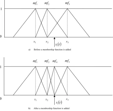
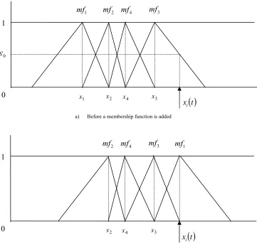
• Only triangular membership functions are generated and only 2 membership functions are allowed to overlap to increase the interpretability of generated fuzzy controllers.
• High-gain observers are used when not all the states are measurable and the design of observers is completely separated from the design of controllers.
• An approximation error estimator and an automatic switching mechanism can be used to further increase the robustness and computational efficiency.
The stability of the overall system, especially when the structure changes, is guaranteed using the Lyapunov stability technique. The overall system is stable in the sense that all the variables are bounded (including number of rules generated) and the tracking error is uniformly ultimately bounded. The proposed control algorithms are implemented in Matlab and Simulink for ease of simulation and practical application. Numerous simulation examples are performed to demonstrate the theoretical results.
The proposed control scheme makes practical application of AFC easier. Designers need to specify only a few design parameters and no longer have to specify the controller structure by trial and error. A simulation or application can be quickly and easily implemented using the developed controllers in Simulink.
Publications
As part of this research, the following papers have been published: Journal papers:
• P.A. Phan, and T.J. Gale, “Two-mode adaptive fuzzy control with approximation error estimator”, IEEE Transactions on Fuzzy Systems, volume 15 (5), pp 943-955, Oct. 2007.
• P.A. Phan, and T.J. Gale, “Direct adaptive fuzzy control with less restrictions on the control gain”, International Journal of Control, Automation, and Systems, Vol 5 No 6 Dec 2007, in press.
• P.A. Phan, and T.J. Gale, “Direct Adaptive Fuzzy Control with a Self-Structuring Algorithm”, Fuzzy Sets and Systems, in press.
Conference papers:
• P. A Phan, and T.J. Gale, ‘Stable Adaptive Fuzzy Controller with Approximation Error Estimators’, Proceedings of The 2nd International Conference on Artificial Intelligence in Science and Technology, Hobart, Tas. Australia, 295-300 (2004)
• P.A. Phan, and T.J. Gale, “Adaptive fuzzy control: approximation error estimator approach”, 23rd IASTED
International Conference on Artificial Intelligence and Applications, Innsbruck, Austria, 2005.
Acknowledgements
I would like to thank my supervisor, Dr. Timothy J Gale, for his endless guidance, support and friendship throughout the duration of the research. He was always there whenever I needed help.
I would also like to thank my associate supervisors, Dr. Bernardo A Leo de La Barra and Prof Michael Negnevitsky, for their advices and help in Control and Artificial Intelligence.
Most importantly, I would like to thank my family for their love and support. Without them, I would not have completed this project.
Table of Contents
ABBREVIATIONS ...9
1. CHAPTER 1 INRODUCTION ...10
1.1. INTRODUCTION...10
1.2. ADAPTIVE FUZZY CONTROL...10
1.2.1. What is adaptive fuzzy control? ...11
1.2.2. Why adaptive fuzzy control? ...11
1.2.3. Relationship between adaptive fuzzy control and adaptive neural network control ...13
1.3. MOTIVATION AND OBJECTIVES...13
1.4. OUTLINE OF THE THESIS...14
1.5. CONCLUSION...16
2. CHAPTER 2 GENERAL LITERATURE REVIEW AND PRELIMINARIES ...17
2.1. INTRODUCTION...17
2.2. A REVIEW ABOUT THE DEVELOPMENT OF ADAPTIVE FUZZY CONTROL...17
2.2.1. Structure...17
2.2.1.1. Direct AFC ...17
2.2.1.2. Indirect AFC...18
2.2.1.3. AFC combined with other controllers ...18
2.2.2. Different classes of nonlinear systems ...20
2.2.2.1. Affine and non-affine nonlinear systems...20
2.2.2.2. Strict-feedback and pure-feedback nonlinear systems ...22
2.2.2.3. SISO and MIMO nonlinear systems...24
2.2.2.4. State-feedback and output feedback nonlinear systems...25
2.2.2.5. Continuous and discrete systems ...25
2.2.3. Adaptive mechanism of fuzzy systems ...26
2.2.3.1. Only parameters are tuned ...26
2.2.3.2. Both parameters and structure are adjusted ...26
2.3. PRELIMINARIES...27
2.3.1. Fuzzy system and neural network ...27
2.3.2. Concepts of stability and boundedness ...27
2.3.2.1. Stability definitions ...28
2.3.2.2. Boundedness definitions...29
2.3.3. Lyapunov stability theorem ...29
2.3.3.1. Conditions for stability ...30
2.3.3.2. Conditions for boundedness ...31
2.3.4. Universal approximation properties ...31
2.3.4.1. Universal approximation property for zero-order Takagi-Sugeno fuzzy systems...31
2.4. BASIC INDIRECT ADAPTIVE FUZZY CONTROL FOR SISO AFFINE NONLINEAR SYSTEMS...33
2.5. CONCLUSION...37
3. CHAPTER 3 TWO-MODE INDIRECT ADAPTIVE FUZZY CONTROL WITH APPROXIMATION ERROR ESTIMATOR...39
3.1. INTRODUCTION...39
3.2. LITERATURE REVIEW...39
3.3. TWO-MODE ADAPTIVE FUZZY CONTROL WITH APPROXIMATION ERROR ESTIMATOR...40
3.4. APPLICATIONS...45
3.4.1. Control of an inverted pendulum ...45
3.4.2. Control of a Chua’s chaotic circuit...47
3.5. CONCLUSION...49
4. CHAPTER 4 DIRECT ADAPTIVE FUZZY CONTROL WITH LESS RESTRICTION ON THE CONTROL GAIN ...54
4.1. INTRODUCTION...54
4.2. LITERATURE REVIEW...54
4.3. DIRECT ADAPTIVE FUZZY CONTROL WITH LESS RESTRICTION...56
4.4. APPLICATIONS...62
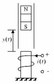
4.4.2. Magnetic levitation system ...63
4.5. CONCLUSION...64
5. CHAPTER 5 SELF-STRUCTURING DIRECT ADAPTIVE FUZZY CONTROL ...69
5.1. INTRODUCTION...69
5.2. LITERATURE REVIEW...69
5.3. SELF-STRUCTURING DIRECT ADAPTIVE FUZZY CONTROL FOR AFFINE NONLINEAR SYSTEMS.71 5.3.1. Description of the self-structuring algorithm...72
5.3.1.1. Criteria for rule generation ...73
5.3.1.2. Adding a membership function and its related rules when the ε-completeness is not satisfied ...73
5.3.1.3. Replacing a membership function and its related rules when the ε -completeness is not satisfied ...75
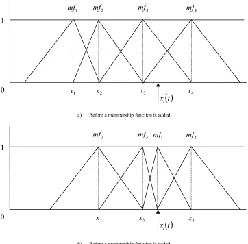
5.3.1.4. Adding a membership function and its related rules when eTPbC is equal to or larger than threshold error_ ...76
5.3.1.5. Replacing a membership function and its related rules when the error measurement C T b P e is equal to or larger than error _threshold ...78
5.3.1.6. Parameters ...79
5.3.2. SSDAFC ...79
5.3.2.1. When the structure is fixed...80
5.3.2.2. When the structure changes ...81
5.4. EXAMPLES...82
5.4.1. Inverted pendulum...82
5.4.2. Magnetic levitation ...84
5.5. CONCLUSION...85
6. CHAPTER 6 SELF-STRUCTURING DIRECT ADAPTIVE FUZZY CONTROL FOR NON-AFFINE NONLINEAR SYSTEMS...90
6.1. INTRODUCTION...90
6.2. LITERATURE REVIEW...90
6.3. SSDAFC FOR NON-AFFINE NONLINEAR SYSTEMS...92
6.3.1. Existence of an ideal control law ...92
6.3.2. Stability analysis ...93
6.4. EXAMPLES...95
6.4.1. Application 1 ...95
6.4.2. Application 2 ...97
6.5. CONCLUSION...98
7. CHAPTER 7 EXTENSION TO THE CONTROL OF OTHER CLASSES OF SISO NON-AFFINE NONLINEAR SYSTEMS...105
7.1. INTRODUCTION...105
7.2. SSDAFC OF SYSTEMS IN THE FORM (7.2)...106
7.2.1. Control of system (7.2) with strong relative degree ρ =n...107
7.2.2. Control of system (7.2) with strong relative degree ρ <n...107
7.3. SSDAFC OF SYSTEMS IN THE TRIANGULAR FORM (7.3)...108
7.4. OUTPUT FEEDBACK SSDAFC...111
7.5. EXAMPLE...117
7.5.1. Continuously stirred tank reactor (CSTR) system without zero dynamics ...117
7.5.2. Continuously stirred tank reactor (CSTR) system with zero dynamics ...120
7.5.3. Third-order system in triangular form (7.3)...122
7.6. CONCLUSION...124
8. CHAPTER 8 MATLAB IMPLEMENTATION ...133
8.1. INTRODUCTION...133
8.2. PROGRAMMING...133
8.3. ADAPTIVE FUZZY CONTROL SIMULINK LIBRARY...134
8.3.1. DAFC block ...134
8.3.3. High-gain observer block...137
8.4. AFC SIMULATION...138
8.4.1. Create a Simulink model for the AFC application ...138
8.4.2. Design the fuzzy system that is used as the initial controller ...139
8.4.3. Load the controller’s parameters...140
8.4.4. Perform simulation ...140
8.5. REAL-TIME AFC...141
8.6. CONCLUSION...143
9. CHAPTER 9 DISCUSSION AND CONCLUSION...144
9.1. DISCUSSION...144
9.1.1. Main contributions ...144
9.1.2. Limitations ...145
9.1.3. Future research...145
9.2. CONCLUSION...146
APPENDIXES...147
APPENDIX 3.A...147
APPENDIX 3.B...151
APPENDIX 4.B...152
APPENDIX 6.A...154
Abbreviations
AFC: Adaptive Fuzzy Control AIC: Adaptive Intelligent Control
ANNC: Adaptive Neural Network Control CSTR: Continuous Stirred Tank Reactor FLC: Fuzzy Logic Controller
GUI: Graphical User Interface MIMO: Multi Input Multi Output NN: Neural Network
SISO: Single Input Single Output
SSAFC: Self-Structuring Adaptive Fuzzy Control SSDAFC: Self-Structuring Adaptive Fuzzy Control
1. Chapter 1
INTRODUCTION
1.1. Introduction
This chapter introduces the thesis and adaptive fuzzy control (AFC), giving a formal definition of AFC and its advantages, then the motivations and objectives of the research. Finally, the outline of the thesis is given, including how the thesis will be organised, what will be presented in each chapter and how they are linked together. 1.2. Adaptive fuzzy control
The early 1990s have witnessed a rapid growth of successful applications of fuzzy logic to automatic control. Examples of such applications are washing machines, electronically stabilized camcorders, auto-focus cameras, air conditioners, automobile transmissions, and subway trains [1]. Indeed, Fuzzy Logic Controllers (FLCs) offer an alternative to the control of complex nonlinear systems that are not easily controlled by conventional automatic control methods as they provide a framework to incorporate linguistic fuzzy information from human experts while not requiring a mathematical model of the plant. However, there is lack of mathematical analysis of stability, robustness, and systematic design procedure. This substantially restricts the application domain of FLCs.
On the other hand, adaptive control has a long history of intense activities involving stability proof, robustness design, and performance analysis [2]. The advances in stability theory and the progress of control theory in the 1960s have improved the understanding of adaptive control. In the mid 1980s, research of adaptive control mainly focused on robustness in the presence of unmodeled dynamics and bounded disturbances. Motivated by the early success of adaptive control of linear systems, the extension to nonlinear systems has been investigated from the end of 1980s to early 1990s. Thus, adaptive control offers powerful mathematical tools to the analysis of stability and robustness of nonlinear control systems.
the stability and robustness of conventional adaptive controllers. Formal definition of adaptive fuzzy control is given next.
1.2.1. What is adaptive fuzzy control?
Wang defines an adaptive fuzzy system as a fuzzy logic system equipped with a training algorithm, where the training algorithm adjusts the parameters (and the structures) of the fuzzy logic system based on numerical information. According to this definition, neuro-fuzzy systems, in which fuzzy systems are represented by neural networks, are also adaptive fuzzy systems.
An adaptive fuzzy controller can be defined as a controller, in which adaptive fuzzy systems are employed and adaptive control theory is used to derive training algorithms such that stability and performance of the closed-loop system are guaranteed.
Lyapunov stability techniques play a critical role in the design and stability analysis of the adaptive systems [2]. A Lyapunov function candidate is a mathematical function designed to provide a simplified scalar measure of the control objectives. The control objectives are met when the chosen Lyapunov function is driven to zero. More details about Lyapunov stability are given in chapter 2. In adaptive fuzzy control systems, stability is investigated by studying the behaviour of some Lyapunov function candidates.
In summary, a controller is called an adaptive fuzzy controller if it possesses both of the following features:
• Adaptive fuzzy systems are employed
• Lyapunov stability technique is used to derive training algorithms to guarantee the stability of the closed-loop system.
1.2.2. Why adaptive fuzzy control?
The advantage of AFC, combining both fuzzy control and adaptive control, includes the followings.
• Fuzzy control provides universal nonlinear approximators. Fuzzy systems are nonlinear universal approximators. In conventional linear robust adaptive control studies, linear approximators are used to approximate some unknown functions that are assumed to be linear. Using fuzzy systems in adaptive control relaxes the assumption that the unknown function must be linear. Thus, it provides an extension to create nonlinear robust control schemes where there is no need to assume that the plant is a linear parameterization of known nonlinear functions [3].
• Fuzzy control is easy to understand. Because fuzzy control emulates human control strategy, its principle is easy to understand for noncontrol specialists. During the past two decades, conventional control theory has been using more and more advanced mathematical tools. This results in fewer and fewer practical engineers who can understand the theory. Therefore, practical engineers tend to use approaches which are simple and easy to understand. Fuzzy control is such an approach [1].
• Fuzzy control is simple to implement. Fuzzy logic systems, which are the heart of fuzzy control, possesses a high degree of parallel implementation. Many fuzzy VLSI chips have been developed, which make the implementation of fuzzy controllers simple and fast.
• Fuzzy control is cheap to develop. Because fuzzy control is easy to understand and simple to implement, the software and hardware cost is low. Also, there are a wide range of software tools available for designing fuzzy controllers (e.g. Matlab).
• Adaptive control is a model-free approach. It does not require a mathematical model of the system. Adaptive algorithms are used to adjust the parameters online
in such a way that the control objectives are met. Thus, a mathematical model of the plant is not needed.
adaptive control, Lyapunov stability technique provides the mathematical framework to establish adaptive algorithms that guarantee stability and robustness.
• Adaptive control provides a systematic design approach. There is no standard systematic design procedure in traditional fuzzy control. The tuning of parameters is mostly based on trial and error approach. Thus, it is a time consuming and ill-defined process. Adaptive control provides a systematic design approach, in which parameters and adaptive laws can be chosen explicitly using Lyapunov technique.
1.2.3. Relationship between adaptive fuzzy control and adaptive neural
network control
Adaptive neural network control (ANNC) is a control method, in which neural networks are employed and adaptive control theory is used to derive training algorithms such that stability and performance of the closed-loop system are guaranteed. Thus, compared to AFC, the main difference is that neural networks are used, instead of fuzzy systems, as approximators.
Moreover, it is well known that a fuzzy system can be realized by a neural network. Many ANNC schemes can be converted to AFC schemes and vice versa. Therefore, it would be inadequate to survey only AFC and ignore ANNC.
In subsequent chapters, ANNC is also considered and is mentioned when it is relevant. The term “adaptive intelligent control” (AIC) will be used to refer to both AFC and ANNC.
1.3. Motivation and Objectives
With the advantages mentioned above, AFC is a very good candidate for control of uncertain nonlinear dynamic systems. However, there are still some drawbacks that obstruct the practical application of AFC.
Other drawbacks include restrictions on the classes of applicable nonlinear systems, constraints on the design parameters that are hard to determine in practice, the complexity of controllers for nonlinear systems in triangular forms, etc.
With the desire to make AFC easier for practical application, the objectives are as follows.
Objectives:
i. Develop a novel online self-structuring AFC scheme that is applicable for a wide range of continuous SISO nonlinear systems.
ii. Propose solutions to overcome drawbacks such as:
Improve computational efficiency by proposing 2-mode adaptive fuzzy control
Relax the extra restrictions of the direct adaptive fuzzy control
Reduce the complexity of the control of nonlinear systems in triangular form
iii. Develop implementation software in order to make simulation and practical application of the proposed AFC scheme fast and easy.
To achieve these objectives, the rest of the thesis is carried as follows. 1.4. Outline of the thesis
Chapter 2 provides a general literature review and mathematical preliminaries. First, we give a brief survey about the development of AFC. Then, some required mathematical preliminaries are given. Finally, basic concepts of AFC (such as ideal control, minimum approximation error, ideal parameters, etc. and how the stability analysis and adaptive laws are derived using Lyapunov stability theorem) are introduced through a simple AFC scheme, basic indirect adaptive fuzzy control for affine nonlinear systems. The shortcomings of this basic AFC scheme are also discussed.
In addition to a general literature review in chapter, there is a separate literature review for each major topic (chapters 3, 4, 5, 6, 7).
switching mechanism improves the computational efficiency in cases where the controlled plants satisfy certain conditions.
Direct AFC is simpler than indirect AFC but it normally requires more restrictions on the control gain than the indirect one. This limits the application of direct AFC in practice. In chapter 4, we propose a direct AFC scheme with less restriction. By using an extension of the approximation theorem, we show that direct AFC actually requires the same restrictions as the indirect one. Also, the proposed control scheme employs a modified adaptive law that guarantees explicit boundedness of adaptive parameters and control action.
In chapter 5, based on the direct AFC scheme proposed in chapter 4, we propose a self-structuring direct AFC scheme for SISO affine nonlinear systems. Compared to some existing algorithms, the proposed self-structuring algorithm is relatively simpler and also guarantees explicit boundedness of the number of rules generated. Only triangular membership functions are generated and only 2 membership functions are allowed to overlap to increase the interpretability of generated fuzzy controllers.
In chapter 6, we extend the result of chapter 5 to a class of non-affine nonlinear systems. By using the implicit function theorem and an extension of the approximation theorem, we show that the AFC scheme proposed in chapter 5 can also be applied to non-affine nonlinear systems.
In chapter 7, we further extend the result to larger classes of nonlinear systems. By using the concepts of Lie derivative and strong relativity, a wider class of non-affine nonlinear systems and a class of nonlinear systems in triangular systems can be transformed to the form in chapter 6. Thus, the AFC scheme proposed in chapter 5 can also be applied to these classes of nonlinear systems. For the class of nonlinear systems in triangular systems, this approach requires only one fuzzy system (unlike the back-stepping approach where one fuzzy system is needed at each step). The approach requires the output and its derivatives, which sometimes are not available for measurement. In this case, high-gain observers are proposed to estimate the derivatives. The design of observers is completely separated from the design of controllers.
mouse operations, a simulation or real-time application of self-structuring AFC can be performed quickly and easily.
Chapter 9 presents discussion and conclusions. 1.5. Conclusion
2. Chapter 2
GENERAL LITERATURE REVIEW AND PRELIMINARIES
2.1. Introduction
This chapter provides background for the thesis. First, a review is presented in section 2.2 to give a general picture about the development of AFC in the past decade. Then, important mathematical background such as stability concept and Lyapunov stability technique is presented in section 2.3. Finally, the basic framework of AFC is introduced in section 2.4 through a simple example of indirect AFC of affine nonlinear systems.
2.2. A review about the development of adaptive fuzzy control
From the early 1990s, adaptive fuzzy control has been an active research area. Many researchers have contributed their work to the field. A great number of different control approaches, methods, schemes, and control applications have been published in various books, journals, and conferences. Thus, providing a complete description of adaptive fuzzy control in a single context is impossible. In this section, a brief review is given in order to demonstrate the wide range of adaptive fuzzy control schemes available in the literature, from different configuration structures, applicable classes of nonlinear systems, to adaptive mechanisms of fuzzy systems.
2.2.1. Structure
In their simplest forms, adaptive fuzzy controllers are constructed only by adaptive fuzzy systems. They can be classified into two categories: direct and indirect adaptive fuzzy control.
2.2.1.1. Direct AFC
2.2.1.2. Indirect AFC
Unlike direct adaptive fuzzy controllers, indirect adaptive fuzzy controllers use adaptive fuzzy logic systems to model the plant and construct the controllers assuming that the fuzzy logic systems represent the true plant. Indirect adaptive fuzzy controllers have been presented in [4-9].
2.2.1.3. AFC combined with other controllers
Pure direct and indirect adaptive fuzzy controls are simple, but they also have disadvantages. Thus, in the later years, it is often that adaptive fuzzy control is combined with other control techniques.
• Direct AFC combined with indirect AFC: [10-13] propose hybrid direct and indirect adaptive fuzzy control schemes in which the control output is the weighted average of a direct and an indirect adaptive fuzzy controllers. This combination provides a framework to incorporate both linguistic knowledge describing the plant behaviour and the control actions.
• AFC combined with another controller to compensate for approximation error: In general, there exist approximation errors when approximating nonlinear functions by fuzzy systems. These approximation errors may effect and deteriorate the stability and performance of adaptive fuzzy control systems. To overcome this problem, previous researchers have proposed combining AFC with another controller. [14] proposes a control scheme in which an indirect adaptive fuzzy controller is combined with a fuzzy sliding mode controller. The fuzzy sliding mode controller is designed to compensate for the approximation errors. [15-20] propose adaptive fuzzy control with a variable structure control term. The variable structure control term is designed using some known bounds of approximation errors. The term is then added to the control output to compensate for the effect of approximation errors. However, the bounds of approximation errors are normally hard to obtain in practice. Thus, they take a step further by proposing some adaptive mechanisms to estimate these bounds online [21, 22].
difficulty. The only variable needed to be measured is output of the system. Many adaptive fuzzy control schemes based on output feedback control have been proposed in the literature: [16, 23].
• AFC combined with H∞ control: External disturbances play an important
role in real control applications. They not only deteriorate control performance but also may cause instability. H∞ optimal control is a
technique used in traditional control theory to minimize the effect of external disturbances. [24-30] use adaptive fuzzy control combined with
∞
H control technique to attenuate the effect of disturbances.
• AFC combined with a supervisory control: An adaptive fuzzy controller sometime does not adapt fast enough. It leads to the state variables of the controlled system moving outside of a desired constraint set. This problem can be solved by increasing adaptive gains. However, adaptive gains cannot be too large. Increasing adaptive gains increases sensitivity to noise, leading to chattering of control output. Thus, to keep the state variables of the system under control in a desired constraint set without the need of large adaptive gains, some researchers [1, 13, 31, 32] propose adaptive fuzzy control combined with a supervisory control. This supervisory control is also a variable structure control term, which is designed using knowledge of the bounds of the unknown nonlinear functions. When the state variables are well inside the constraint set, the supervisory control is zero. When the state variables tend to move outside of the desired boundaries, the supervisory control begins to operate to force the states to stay in the constraint set.
both the effects of approximation errors and external disturbances can be attenuated to any prescribed level.
In general, adaptive fuzzy control combined with other control schemes overcome disadvantages existing in pure direct and indirect adaptive fuzzy control. However, they are more complicated in both theoretical analysis and implementation. Thus, for a particular application, it is up to control designers to decide when it is necessary to combine adaptive fuzzy control with another control technique.
2.2.2. Different classes of nonlinear systems
In the theory of nonlinear control, the control of different classes of nonlinear systems has been considered. Different classes of nonlinear systems have different characteristics, and thus require different control techniques. Some well-established techniques are available for different classes of nonlinear systems. For example, linearizable nonlinear systems can be treated using feedback linearization techniques. Nonlinear systems in strict-feedback forms can be treated using backstepping design. Nonlinear systems, in which not all the state variables are measurable, can be dealt with using output feedback control, etc. These results in nonlinear control have inspired researchers to propose a number of adaptive fuzzy control schemes for these classes of nonlinear systems based on the available techniques.
Here, we review AFC schemes in terms of the nonlinear classes that they can be applied to.
2.2.2.1. Affine and non-affine nonlinear systems
• Affine nonlinear systems
Under some geometric conditions, the input-output response of a class of single input-single-output (SISO) nonlinear systems can be rendered to the following
Brunovsky form [2]:
( ) ( )
( )
=
+ +
=
− =
= +
1
1 1 1
x y
t d u x g x f x
,n , ,i x x
n i i
&
K &
( )
2.1where x=
[
xq,x2,K,xn]
T ∈Rn, u∈R, y∈R are the state variables, systemNonlinear systems that can be represented in this form are also known as affine nonlinear systems as the systems are linear in the input variables.
If f
( )
x and g( )
x are known, the feedback linearization technique can be used to design a controller. The most common control structure is( )
x[
f( )
x v]
gu = 1 − +
( )
2.2where v is a new control variable. In cases where f
( )
x and g( )
x are unknown, adaptive fuzzy control has been proposed.[1, 4-7] propose indirect adaptive fuzzy control schemes for affine nonlinear systems, in which two adaptive fuzzy systems fˆ
( )
xθ f and gˆ( )
xθg are used to approximate f( )
x and g( )
x respectively. Lypapunov stability analysis is used to derive the adaptive laws and to guarantee the control objectives. In these approaches, it should be noted that additional precautions are required to avoid possible singularities of the controllers (i.e., gˆ( )
xθg =0). For instance, in Wang [1], a projection algorithm is proposed for adjusting θg to avoid singularities.[24, 25, 32] propose direct adaptive fuzzy control schemes for nonlinear affine systems. In these schemes, only one adaptive fuzzy system uˆ
(
x,vθ)
is used to approximate the control( )
x[
f( )
x v]
gu= 1 − + . Direct adaptive fuzzy control schemes avoid control singularity problem completely. However, compared to indirect schemes, more restrictions on g
( )
x are normally required. More discussion on the restrictions of direct AFC will be given in chapter 4.• Non-affine nonlinear systems
Non-affine nonlinear systems is a broader class of nonlinear systems, whose input variables may not be expressed in an affine form. A SISO non-affine nonlinear system is defined as:
( )
= =
− =
= +
1 1
,
1 1
x y
u x f x
,n , ,i x x
n i i
&
K &
where x=
[
xq,x2,K,xn]
T ∈Rn, u∈R, y∈R are the state variables, system inputand output, respectively; f
( )
x,u is a unknown smooth function. It can be seen that affine nonlinear systems are a special case of this class of nonlinear systems.In the past five years, researchers have proposed different AFC schemes [2, 33-38] for non-affine nonlinear systems. Because the control input does not appear linearly, the well-known feedback linearization technique is not applicable. Adaptive fuzzy control of non-affine nonlinear systems is more difficult and challenging. In general, more advanced mathematical techniques are required.
2.2.2.2. Strict-feedback and pure-feedback nonlinear systems
• Strict-feedback nonlinear systems
A large number of practical nonlinear systems can be expressed in or transformed into a special state-space form called strict-feedback form:
( )
( )
( )
( )
=
≥ +
=
− ≤ ≤ +
= +
1
1
x y
2 n ,
1 1
,
u x g x f x
n i x
x g x f x
n n n n n
i i i i i i
& &
( )
2.4where
[
]
T ii
i x x x R
x = 1, 2,K, ∈ , i=1,K,n, u∈R, y∈R are state variables, system
input and output, respectively. fi
( )
• and gi( )
• , i=1Kn, are smooth unknownfunctions. The control objective is to determine the control input u such that output
y tracks a reference signal r as close as possible.
However, a major constraint of traditional adaptive backstepping technique is that unknown functions fi
( )
xi and gi( )
xi , i=1Kn must be “linear in the unknownparameters”. With the use of neural networks and adaptive fuzzy systems, this assumption can be relaxed.
Adaptive neural network backstepping control has been proposed in [39-42]. Neural networks are used in each step to approximate the unknown functions. A drawback of these adaptive neural network backstepping control schemes is the problem of “explosion of complexity”, the complexity of controllers grows drastically as the order n of the system increases.
This explosion of complexity is caused by the need to estimate derivatives of certain nonlinear functions [43]. At each step, to estimate this derivative, partial derivatives are need to be computed and they are also need to be used as inputs to neural networks. The number of partial derivatives increases drastically after each step, and thus increases drastically the complexity of controllers. To overcome this problem, [43] proposes a dynamic surface control technique, in which a first-order filter is introduced at each step to avoid the need to estimate derivatives of certain nonlinear functions.
Recently, adaptive intelligent control has also been developed for discrete strict-feedback systems. [44] proposes a state-strict-feedback adaptive NN control scheme using backstepping, and an output-feedback adaptive NN control scheme using a diffeomorphism transformation. The MIMO case has also been considered in [45, 46].
• Pure-feedback nonlinear systems
Pure-feedback systems are a broader class of low-triangular-structured nonlinear systems, which is given in a general form as:
(
)
(
)
= =
− =
= +
1
1 ,
1 , , 1 , ,
x y
u x f x
n i
x x f x
n n n
i i i i
&
K &
( )
2.5where
[
]
T ii
i x x x R
x = 1, 2,K, ∈ , i=1,K,n, u∈R, y∈R are state variables,
system input and output, respectively. fi
(
xi,xi+1)
, i=1Kn, are smooth functions.( )
2.5 is more difficult than control of strict-feedback systems( )
2.4 . Few results of controlling pure-feedback systems have been reported in the literature [34, 47].[47] proposes adaptive neural control of pure-feedback systems by combining backstepping, input-to-state stability analysis, and the small-gain theorem. The proposed control scheme, however, also suffers from the problem of “explosion of complexity”. [34] proposes adaptive neural network control using Nussbaum-Gain functions and the idea of backstepping. A drawback of this approach is the closed-loop system has wild transient performance.
2.2.2.3. SISO and MIMO nonlinear systems
Inspired by the results for SISO nonlinear systems, researchers have also developed adaptive intelligent control for uncertain MIMO nonlinear systems.
Control of uncertain MIMO nonlinear systems, in general, is more difficult. It is due to the difficulties in dealing with the couplings in input matrices and interconnections between subsystems.
[48] proposes adaptive fuzzy control for a class of MIMO nonlinear systems, which consists of affine subsystems. And it is assumed that there is no input coupling and the system interconnections are bounded with known constants.
[49-53] present adaptive fuzzy/neural control for a class of MIMO square nonlinear plants, in which the bounding restrictions on the system interconnections are relaxed. However, it is required that the number of inputs equals the number of outputs and the inputs are also in affine forms.
In [54, 55] adaptive neural network controllers were proposed for some special classes of MIMO nonlinear robotic systems, using several nice properties of the robotic systems.
In [56], an adaptive neural control approach was proposed for a class of MIMO nonlinear systems with a triangular structure in control inputs.
In [57], adaptive neural control is proposed for two classes of uncertain MIMO nonlinear systems in block-triangular forms, which consists of couplings in the inputs as well as in the system interconnections without any bounding restrictions.
2.2.2.4. State-feedback and output feedback nonlinear systems
State-feedback control deals with systems in which it is assumed that all the state variables are available for measurement. In practice, it is sometime difficult or impossible to measure all the state variables. Output-feedback control is the control of systems in which only outputs are required to be available for measurement.
For affine and nonaffine SISO nonlinear systems, [44, 58] propose adaptive NN output feedback control using high gain observers to estimate the required derivatives of the outputs. Due to the use of high gain observers, a peaking phenomenon in the transient behaviour may occur. To overcome such a problem, saturation methods introduced in [59, 60] may be used. [61, 62] propose using linear observers to observe the error dynamics. [38] proposes a non-observer approach, in which input/output history are used as inputs to NNs instead of the derivatives of the system output.
Adaptive intelligent output feedback control for wider classes of nonlinear systems has also been considered. MIMO cases are considered in [46, 63, 64]. Systems with zero dynamics are treated in [65, 66].
2.2.2.5. Continuous and discrete systems
Since most controllers are implemented using digital computers, control in discrete time domain is an important topic. Adaptive intelligent control for discrete-time nonlinear systems has also received attention from researchers. Due to the difficulties in discrete-time systems, such as the noncausal problem in backstepping design, discrete-time domain methods are much less common than those in the continuous domain [46].
For SISO discrete time systems, [67, 68] propose adaptive intelligent control for a class of discrete affine nonlinear systems. [69] proposes both state and output feedback controls for a class of discrete-time systems with general relative degree and bounded disturbances. For a class of discrete-time systems in strict feedback form, an effective backstepping design method was proposed in [70].
2.2.3. Adaptive mechanism of fuzzy systems
2.2.3.1. Only parameters are tuned
In adaptive intelligent control, intelligent systems (i.e. neural networks, neural-fuzzy systems, or adaptive neural-fuzzy systems) are employed to approximate some unknown functions. To guarantee the stability, parameters of intelligent systems are tuned online.
In an intelligent system, there are two type of parameters: linear parameters and nonlinear parameters. For example, consequents of a fuzzy system are linear parameters, whereas input membership function parameters (centers and variances) are nonlinear parameters. For a multi-layer neural network, synaptic weights of the output layer are linear parameters, whereas weights of the hidden layers are nonlinear parameters.
Most of the work reported in the literature employs intelligent systems with linear tuneable parameters. Fewer results are available for intelligent systems with nonlinear tuneable parameters. [2] proposes adaptive control using multi-layer neural networks, in which the weights of hidden layers are nonlinear parameters. [3, 72, 73] propose adaptive fuzzy control, in which the input membership function parameters are also tuned.
Linear parameterized intelligent systems are simpler to tune and to analyze. They, however, suffer “the curse of dimensionality”, their size tend to increase exponentially with the dimension of the input space. Nonlinear parameterized intelligent systems are normally smaller (in term of size) to achieve the same approximation accuracy and they are global approximators. However, the learning speed is slower and analysis is more difficult. Thus, it normally depends on a particular application to decide which type is more suitable.
2.2.3.2. Both parameters and structure are adjusted
Few attempts to develop self-structuring intelligent systems for adaptive control have been reported. Park et al [37, 74] proposes using self-structuring adaptive fuzzy control, in which rules are added to the rule base as the input space is explored. Gao [51] proposes using self-organising adaptive fuzzy neural control, which is able to add or delete rules from the rule base. Park et al [36] proposes self-structuring adaptive neural network control , in which a neuron in the hidden layer splits into two if a certain condition is satisfied.
However, there exist some limitations in the above methods. Even if self-structuring algorithms are presented, stability analysis is only performed for the fixed-structured case. There is no discussion on the effect of the self-structuring algorithms on the stability. [36, 37, 74] do not propose any algorithm to limit the size of the intelligent systems. Thus, there is a risk that the intelligent systems will exceed the hardware capability if initial performance is poor. Gao [51] uses large matrix manipulation and an Error Reduction Ratio technique to prune rules. Thus, the approach is complicated and computationally inefficient. Self-structuring adaptive intelligent control is, therefore, still an open research topic.
2.3. Preliminaries
2.3.1. Fuzzy system and neural network
The required knowledge includes basic topics such as:
• Fuzzy set theory
• Fuzzy systems ( Mandani and Takagi-Sugeno types)
• Fundamentals of neural networks
• Backpropagation and related training algorithms
There are numerous books in the literature that cover these areas such as [75-77]. Thus, we will not re-present these areas here.
2.3.2. Concepts of stability and boundedness
[2, 3, 78] Consider the autonomous nonlinear system described by
( )
x fx&= , n
R f
2.3.2.1. Stability definitions
Definition 2.1 A state x∗ is an equilibrium state (or equilibrium point) of the system
( )
2.6 , if once x( )
t is equal to x∗, it will remain equal to x∗ forever. In mathematical terms, that means the vector x∗ satisfies:( )
x∗ =0f
Without the loss of generality, we may assume the origin x∗ =0 is an equilibrium point.
Definition 2.2 The equilibrium point x∗ =0 is said to be Lyapunov stable if, for any given ε >0, there exists a positive δ
( )
ε such that if( )
0 <δ( )
εx ,
then x
( )
t <ε, ∀t≥0.Otherwise, the equilibrium point is unstable.
Definition 2.3 The equilibrium point x∗ =0 is said to be asymptotically stable if it is Lyapunov stable and there exists δ such that if
( )
0 <δx ,
then lim
( )
=0∞ → x t
t .
Definition 2.4 The equilibrium point x∗ =0 is said to be exponentially stable if it is asymptotically stable and there exist α,β,δ >0 such that if
( )
0 <δx ,
then x
( )
t ≤α x( )
0 e−βt, for t≥0.Conceptually, the meanings of the above terms are the following:
• Lyapunov stability of an equilibrium point means that solutions starting “close enough” to the equilibrium point (within the distance δ from it) remain “close enough” forever. Note that this must be true for any ε that one may want to choose.
• Exponential stability means that solutions not only converge, but in fact converge faster than or at least as fast as a particular known rate
( )
te
x β
α −
0 .
2.3.2.2. Boundedness definitions
Definition 2.5 A solution x
( )
t is bounded if there exists a β >0, that may depend on each solution, such that( )
t < βx for all t≥0.
Definition 2.6 The solutions x
( )
t are uniformly bounded if for any α>0, there exists β( )
α such that if( )
0 <αx ,
then x
( )
t <β( )
α for all t≥0.Definition 2.7 The solutions x
( )
t are uniformly ultimately bounded if for any 0>
α , there exist β and T
(
β,x( )
0)
such that if( )
0 <αx ,
then x
( )
t <β for all t≥T(
β,x( )
0)
.Definition 2.8 The solutions x
( )
t are semi-globally uniformly ultimately bounded if for any Ω, a compact subset of ℜn, there exist β and T(
β,x( )
0)
such that if( )
0 ∈Ωx ,
then x
( )
t <β for all t≥T(
β,x( )
0)
.2.3.3. Lyapunov stability theorem
Definition 2.9 A continuous function γ :ℜ→ℜ+ is said to belong to class К if
• α
( )
0 =0.• α
( )
r →∞ as r→∞.• α
( )
r >0 ∀r>0.• locally positive definite if there exists a class К function α
( )
• such that( )
x t( )
xV , ≥α
for all t≥0 and x in the neighbourhood Ν of the origin ℜn. • positive definite if Ν=ℜn.
• (locally) negative definite if −V is (locally) positive definite.
• (locally) decrescent if there exists a class К function β
( )
• such that( )
x t( )
xV , ≤β
for all t≥0 and x in (the neighbourhood Ν of the origin) ℜn.
2.3.3.1. Conditions for stability
Theorem 2.1 Lyapunov Theorem
Given the non-linear dynamic system
( )
x tf
x&= , ,
( )
00 x
x =
with an equilibrium point at the origin, and let Ν be a neighbourhood of
the origin, i.e. Ν=
{
x: x ≤ε ,withε >0}
, then the origin 0 is• stable in the sense of Lyapunov if for x∈N, there exists a scalar
function V
( )
x,t such that V( )
x,t >0 and V&( )
x,t ≤0, ∀x≠0.• uniformly stable if for x∈N, there exists a scalar function V
( )
x,t such that V( )
x,t >0 and decrescent and V&( )
x,t ≤0, ∀x≠0.• asymptotically stable if for x∈N, there exists a scalar function
( )
x tV , such that V
( )
x,t >0 and V&( )
x,t <0, ∀x≠0.• globally asymptotically stable if for x∈ℜn, there exists a scalar
function V
( )
x,t such that V( )
x,t >0 and V&( )
x,t ≤0, ∀x≠0.• uniformly asymptotically stable if for x∈N, there exists a scalar
function V
( )
x,t such that V( )
x,t >0 and decrescent and( )
x,t <0• globally, uniformly, asymptotically stable if x∈ℜn, there exists a
scalar function V
( )
x,t such that V( )
x,t >0 and decrescent and( )
x,t <0V& , ∀x≠0.
• exponentially stable if there exist positive constants α, β , γ such
that ∀x∈N, α x 2 ≤V
( )
x,t ≤β x 2 and V&( )
x,t ≤−γ x 2.• globally exponentially stable if there exist positive constants α,
β , γ such that ∀x∈ℜn, α x 2 ≤V
( )
x,t ≤β x 2 and( )
2,t x
x
V& ≤−γ .
2.3.3.2. Conditions for boundedness
Uniform ultimate boundedness (UUB) If there exists a function V
( )
x with continuous partial derivatives such that for nS
x∈ ⊂ℜ :
• V
( )
x is positive definite: V( )
x >0, ∀ x ≠0• Time derivative of V
( )
x is negative definite outside of S:( )
x <0V& , ∀x >β,
(
x ≤B)
⇒(
x∈S)
Then the system is UUB and x ≤B, ∀t≥t0 +T .
2.3.4. Universal approximation properties
2.3.4.1. Universal approximation property for zero-order Takagi-Sugeno fuzzy
systems
Consider zero-order Takagi-Sugeno fuzzy systems with point fuzzification method, product-type inference, and center-average defuzzifier.
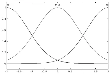
For each a<b, a,b∈R, let α
( )
a,b :R→[0,1] be a membership function such that α( )( )
a,b x ≠0 if x∈( )
a,b and α( )( )
a,b x =0 if x∉( )
a,b . The fuzzy system has the If-Then rule base of the following form:R(i): IF x1 is A1i, and x2 is A2i, and …and xn is Ani, THEN y is θi
where x=(x1,x2,K,xn)T ∈U ⊂Rn and y∈V ⊂R are the crisp input and
( )
(
)
( )
j i j i j ji
j x a a x
A =α 1, 2 for some aij1<aij2, i=1,K,M where M is the number of
rules, j=1,K,n.
i
θ is the system output due to rule R(i).
Then, the output of a Takagi-Sugeno fuzzy system is a weighted average of θi:
∑
∑
∑
= =
= =
=
= M
i i i M
i i
M
i i i
x x
x x
f y
1 1
1
) ( )
( ) ( )
| ( ˆ
ˆ θζ
µ µ θ
θ
( )
2.7in which
∏
( )
=
= n
j
j i j
i x A x
1 ) (
µ , ζi(x)≥0 and ( ) 1
1
=
∑
=M
i i x
ζ .
Theorem 2.2: Universal approximation theorem
For any given real continuous function g on a compact set U ⊂ℜn and arbitraryε >0, if a large enough number of rules is used, there exists a fuzzy logic system f in the form of
( )
2.7 such that( ) ( )
− <ε∈U f x g x x
sup Proof
The proof of this theorem can be found in [1, 3].
Remark 2.1 This theorem justifies that Takagi-Sugeno fuzzy systems with either triangular membership functions or Gaussian membership functions are universal approximators. Thus, in this thesis, we will use both Takagi-Sugeno fuzzy systems with triangular membership functions and the ones with Gaussian membership functions as our fuzzy controllers.
Remark 2.2 This theorem is just an existence theorem. How to determine the sufficient number of rules or how to find such a fuzzy logic system are different questions. We are more interested in answer the question “ How to find a fuzzy logic controller such that the closed-loop system is stable and the tracking error converge
to a small neighbourhood of zero?”.
2.4. Basic indirect adaptive fuzzy control for SISO affine nonlinear systems
As an example, this section shows how the above mathematical tools are used to construct a simple adaptive fuzzy controller for SISO affine nonlinear systems. Consider SISO affine nonlinear systems in the following form:
1 3 2
2 1
) ( ) (
x y
u x g x f x
x x
x x
n
=
+ = = =
& K K & &
( )
2.8where u is the control input; y is the output; f(x) and g(x) are unknown continuous functions; x=(x1,,x2,K,xn)T is the state vector of the system which is assumed available for measurement.
Control objective is to design an adaptive fuzzy controller such that the output )
(t
y of the system follows a continuous reference signal r(t)⊂Cn. Assumptions
To design a controller satisfying the above control objective, the following assumptions are made:
• Assumption 2.1: g(x) is continuous and the sign of g(x) is known for
x
x∈Ω , where Ωx is the controllability region.
Since g(x)≠0 (controllable condition of system
( )
2.8 ) and g(x) iscontinuous for x in the controllability region Ωx, without loss of generality, it can be assumed that g(x)>0 for x∈Ωx.
• Assumption 2.2:Define r=[r&,&r&,&r&&K,r(n−1)]T. We assume that 0
r
r ≤
and r(n) ≤r1 with known constants r0,r1>0. Ideal control
Let e=r−y, e=
(
e,e&,&e&,K,e(n−1))
T, and(
)
T nk k k
k= 1, 2,K, be such that the polynomial s k sn1 k1
n
n + − +K+ is Hurwitz stable. If the functions
( )
x
f and g
( )
xare known, then the control law
( )
x(
f( )
x kTe r( )n)
gapplied to
( )
2.8 results in( ) ( 1)
2 1
−
− −
− = −
= n
n T
n k e ke k e k e
e &K
(
2.10)
which implies that lim =0+∞ → e
t . The control
∗
u is called ideal control.
Certainty equivalent control, direct and indirect AFC
However, f(x) and g(x) are unknown. Thus, we need to employ fuzzy systems to approximate the unknown functions. If we use one fuzzy system to approximate
∗
u , we have direct AFC. If we use two fuzzy systems to model f(x) and g(x), we have indirect AFC. Direct AFC will be discussed in the next chapter. Here, we consider the indirect case.
Employ two fuzzy systems fˆ(x|θf) and gˆ(x|θg) in the form
( )
2.7 to approximate f(x) and g(x) respectively. The resulting control law is( )
(
T n)
f g
c f x k e r
x g
u = − ˆ( | )+ +
) | ( ˆ
1
θ
θ
(
2.11)
is the so-called certainty equivalent control.
Ideal parameters and minimum approximation error
The ideal parametersθ∗f and θ∗g are defined as:
( )
[
x U f x f f x]
f = ∈ x −
∗
) | ( ˆ sup min
arg θ
θ
(
2.12)
( )
[
x U g x g g x]
g = ∈ x −
∗
) | ( ˆ sup min
arg θ
θ
(
2.13)
The minimum approximation error is defined as:( )
(
f x f f x)
f = −
∗
) | (
ˆ θ
ω
(
2.14a)
( )
(
g x g g x)
g = −
∗
) | (
ˆ θ
ω
(
2.14b)
Stability analysis and adaptive laws
Substituting u=uc, adding and subtracting g(x)u∗ to
( )
2.8 , we obtain the error equation( )
(
f)
(
g( )
)
c Tn k e f x f x g x g x u
e( ) =− + ˆ( |θ )− + ˆ( |θ )−
(
2.15)
or in the matrix form( )
(
)
(
( )
)
[
f g c]
C
Ce b f x f x g x g x u
n 3 2 1 C k -k -k -k -1 0 0 0 0 1 0 0 0 0 1 0 = Λ L L M O M M M L L , = 1 0 0 0 M C b .
From
(
2.14)
,(
2.16)
becomes(
)
(
)
[
θ f θf θg θg c]
CωC
Ce b f x f x g x g x u b
e&=Λ + ˆ( | )− ˆ( | ∗) + ˆ( | )− ˆ( | ∗) +
(
2.17)
where the total approximation error ω=ωf +ωguc.From
( )
2.7 ,(
2.17)
can be written as( )
( )
[
φ ζ φ ζ c]
CωT g T
f C
Ce b x x u b
e&=Λ + + +
(
2.18)
where = f − ∗f
f θ θ
φ , = g − ∗g
g θ θ
φ .
Since ΛC is a stable matrix, there exists a unique positive definite symmetric
n
n× matrix P which satisfies the Lyapunov equation:
Q P
P C
T
C + Λ =−
Λ
(
2.19)
where Q is an arbitrary n×n positive definite matrix.To perform the stability analysis, consider the Lyapunov function candidate
g T g g f T f f T e P e
V φ φ
γ φ φ γ 2 1 2 1 2 1 + +
=
(
2.20)
where γf and γg are positive constants. The time derivative of V along the trajectory of
(
2.18)
is( )
[
e Pb x]
[
e Pb( )
x]
b P e e Q e V C T g g T g g C T f f T f f C T T ζ γ θ φ γ ζ γ θ φ γ ω + + + + + − = & & & 1 1 2 1
(
2.21)
where we used
(
2.19)
and ff θ
φ& = & ,
g
g θ
φ& = & . If we choose the adaptive laws
C T f
f γ e Pb
θ& =−
(
2.22)
C T g
g γ e Pb
θ& =−
(
2.23)
then from
(
2.21)
we haveω C T T b P e e Q e
V =− +
2 1