Escort tug at large yaw angle: comparison of CFD predictions with experimental data

ESCORT TUG AT LARGE YAW ANGLE: COMPARISON

OF CFD PREDICTIONS WITH EXPERIMENTAL DATA

David Molyneux, Senior Research Officer, Institute for Ocean Technology, National Research Council Canada, St. John’s, Newfoundland, Canada

&

Neil Bose, Professor of Maritime Hydrodynamics, Australian Maritime College, Launceston, Tasmania, Australia

ABSTRACT

Escort tugs operate at high yaw angles in order to produce forces to steer and stop the vessel they are escorting in an emergency. In this paper, RANS predictions of forces and flow patterns around the hull of an escort tug model are compared with experimental data. Two alternative meshing strategies were used, one using tetrahedral elements with

triangular faces and one using hexahedral elements with quadrilateral faces.

Experiments were carried out with and without the low aspect ratio fin that is typical of many escort tugs. Lift and drag forces were measured experimentally for yaw angles from 15 to 45 degrees. Flow measurements around the tug at 45 degrees yaw were obtained using a stereoscopic particle image velocimetry (PIV) system.

The results from each CFD simulation were compared to the measured flow patterns using a numerical procedure that led to a quantitative measure of the accuracy of the predicted results. The analysis of the flow patterns indicated that the main features of the flow were predicted, and that on average, the predicted velocity magnitudes were within 10% of the measured values. Neither mesh approach had a significant effect on the accuracy of the flow pattern predictions. The hexahedral mesh gave more accurate force predictions that the tetrahedral mesh. Forces were predicted by the CFD code with this mesh to within 5 % of the experimentally obtained values.

1. INTRODUCTION

considered to be the design conditions, and the ‘off-design’ conditions, where these assumptions are no longer valid have seldom been studied. An escort tug is a vessel where ‘off-design’ hydrodynamics are an essential part of the ship’s operational profile (Allan & Molyneux, 2004). In this situation, the tug’s hull and propulsion system are positioned to create a hydrodynamic force, which is used to bring a loaded oil tanker under control in an emergency. The tug is attached to a towline at the stern of the tanker, and by using vectored thrust, it is held at a yaw angle of approximately 45 degrees. The maximum practical speed of operation for escort tugs is about 10 knots. The designs of escort tugs to date have been developed from practical experience and model experiments to measure lift and drag forces. A full understanding of the flow has not been developed, and it is unlikely that escort tugs can be developed to their full potential without this knowledge.

One method of trying to understand the flow around a hull with a large angle of attack (yaw angle) is to use computational fluid dynamics (CFD). The basic equations of fluid motion can be combined with the hull geometry and some assumptions about the

turbulence in the flow to give mathematical predictions of the pressure on the hull surface and the flow vectors within the fluid. Very little numerical analysis has been carried out on the hydrodynamics of hull shapes designed to operate at large yaw angles, and so the accuracy of CFD in these situations is unknown.

(Molyneux and Bose, 2007) concluded that there was very little difference in the predicted flow patterns between an unstructured mesh made from tetrahedral elements and a structured mesh made from hexahedral elements, when each was compared with experiment data. The Series 60 hull was not designed for large angles of attack to the flow and there was no force data available for the hull above 10 degrees of yaw, so the comparison was incomplete.

It was recommended (Molyneux & Bose, 2007) that the conclusions on the best meshing strategy for the Series 60 hull should be checked using hull forms designed to operate at yaw angles over 30 degrees. This paper extends the comparison of forces and flow patterns calculated using tetrahedral and hexahedral CFD meshing strategies to a hull shape designed specifically to operate in ‘off-design’ conditions given by yaw angles up to 45 degrees. Some conclusions are made on the effectiveness of commercial RANS based CFD codes within the design process for ship hulls that are required to operate at large yaw angles.

2. MODEL EXPERIMENTS TO MEASURE HYDRODYNAMIC FORCES

5 0

2 3 6

1

7 8

9

10

Design Waterline

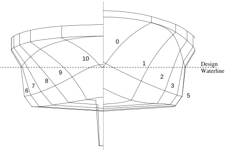
Figure 1, Body plan for tug model, used in PIV experiments.

Design Waterline

A summary of the model geometry is given in Table 1. For this series of experiments the model was always moving with the fin (when fitted) going forwards (although the ship is actually going astern based on conventional definitions of bow and stern). This situation results from the fact that escort tugs have evolved from tractor tugs, which under normal operations sail with the propulsion system at the forward end of the hull. For effective escort mode at high speed, the tug operates in ‘indirect mode’, which is astern by the conventional definition.

Table 1, Summary of principle particulars, escort tug Appendage option Hull only Hull and fin

Lwl, m 38.19 38.19

Bwl, m 14.2 14.2

T (max), m 3.8 6.86

Displacement, tonnes S.W.

1276 1276 Lateral area, m2 125.4 157.1

Experiments to measure hull forces were carried out in the Ice Tank of the National Research Council’s Institute for Ocean Technology (Molyneux, 2003). The objective of these tests was to measure hydrodynamic forces and moments created by the hull and the appendages on a 1:18 scale model of the ship. The range of ship speeds was from 4 to 12 knots (with model speeds based on Froude length scaling). Yaw angle was varied

different hull configurations to be compared, in much the same way as a resistance experiment can give a measure of merit for different hulls at zero yaw angle. The test method was very similar to that proposed by earlier researchers (Hutchison et al., 1993). The fin was at the upstream end of the hull, for all cases when it was fitted. The hull remained in the same orientation when the fin was removed.

The models were fixed at the required yaw angle and measurements were made of surge force, sway force and yaw moment using a Planar Motion Mechanism (PMM). The load measurement system was connected to the tug on an axis along its centreline, at the height of the towing staple on the tug. The model was free to roll about the axis through the towing staple, and free to pitch and heave. Pitch angle, roll angle, heave amplitude and carriage speed were measured, in addition to the surge force Fx and sway force Fy. The model being tested on the PMM frame is shown in Figure 3.

A small negative value of yaw angle (usually five or ten degrees) was used to check the symmetry of the results, and if necessary make a small correction to yaw angle to allow for any small misalignment of the model on the PMM frame. Prior to each days testing, the PMM system was checked using a series of static pulls which included surge only, sway only and combined surge and sway loads. Also individual data points were tared using data values for transducers obtained with the model stationary before the

Figure 3, Model tested on PMM (10 knots)

Forces and moments were measured in the tug-based coordinate system and non-dimensionalized using the coefficients given below

2

5 . 0 AV

F C

L x

l = _{ρ 2}

5 . 0 AV

F C

L y

q = ρ

Cqis the force coefficient normal to the tug centerline (sway) and Clis the force

When the measured force values were non-dimensionalized, the results for all speeds reduced to small variations about a mean value of the coefficient (Molyneux, 2003). This implied that free surface wave effects are small for the range of speeds typically found in escort tug operation. This observation simplified the CFD predictions since only the hull below the design waterline needs to be considered, and the free surface effects can be ignored.

3. CFD PREDICTIONS OF HYDRODYNAMIC FORCES

The surfaces used to construct the 1:18 scale physical model (Molyneux, 2003) were trimmed to the nominal waterline. The trimmed surfaces were imported as IGES files and cleaned up using the utilities available within GAMBIT (Fluent Inc., 2005a), the program used for creating the meshes. Dimensions for the surfaces were originally given in inches at model scale. The mesh was re-scaled in FLUENT (Fluent Inc., 2005b) to have units of metres, model scale and an origin at the leading edge of the waterline for the hull. All dimensions given in this report are metres, model scale.

A rectangular ‘tank’ was constructed around the hull. This had to be a compromise between being large enough that the boundaries had little effect on the results, and small enough that it converged to a solution in a reasonable time. The same domain size was used for tetrahedral and hexahedral meshing strategies. Both meshes were created using

geometry was used for the hull with and without the fin, and so views are shown for the case with the fin only.

Table 2, Summary of mesh dimensions

xmax xmin ymax ymin z max zmin

m m m m m m 7.974 -2.059 4.318 -4.318 0.000 -2.159

3.1 Tetrahedral Mesh

Y Z

X

Figure 4, Tetrahedral mesh for escort tug hull

Y Z

X

3.3 Hexahedral Mesh

The surface file used to create the hexahedral mesh was the same as the one used for the tetrahedral mesh. For the hexahedral mesh the additional step of creating new surfaces so that the hull could be defined completely in four-sided elements was required. This was done within Gambit.

Again the mesh was divided into two regions. One region was close to the hull surface, and one was sufficiently far from the hull surface that flow conditions were not changing significantly. The hull and fluid volume were defined using a more elaborate system of construction planes along the length of the hull, especially close to the bow and the stern. Once the inner mesh was successfully defined, the cells in the planes were extruded to the inlet, outlet and bottom wall boundaries. The mesh was symmetrical about the centreline of the ship. The total number of elements within the mesh was 986,984, which was less than one half of the number used for the tetrahedral mesh. The hexahedral mesh is shown in Figure 5, for the hull surface and the nominal free surface.

3.4 CFD Solver

For both meshes the boundary conditions were set as velocity inlets on the two upstream faces, and pressure outlets at the two downstream faces. The upper and lower boundaries were set as walls with zero shear force. The hull surface was set as a no-slip wall

The CFD solver used was FLUENT 6.1.22. Uniform flow entered the domain through a velocity inlet on the upstream boundaries and exited through a pressure outlet on the downstream boundaries. Flow speed magnitude was set at 0.728 m/s, which corresponded to 6 knots at 1:18 scale, based on Froude length scaling. The fluid used was fresh water.

The angle between the incoming flow and the hull (yaw angle) was set by adjusting the boundary conditions, so that the velocity at the inlet planes had two components. The cosine component of the angle between the steady flow and the centreline of the hull was in the positive x direction for the mesh and the sine component in the positive y direction. The pressure outlet planes were set so that the backflow pressure was also in the same direction. The advantage of this approach was that one mesh could be used for all the yaw angles. Yaw angles from 10 degrees to 45 degrees were simulated.

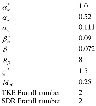
The selection of the turbulence model was based on discussions with experienced users of

Fluent and other CFD codes (Rhee 2005, Turnock, 2006,). The turbulence model used was a κ−ω model with the default parameters given in Table 3. Turbulence intensity and turbulent viscosity ratios were set at 1% and 1 respectively. The flow was solved for the steady state case. The non-dimensional residual for each of the solution variables

(continuity, x, y and z velocity components, κ and ω) were set to 10-3 (default values). All flow conditions reported came to a solution within these tolerances. Results were

Table 3, Parameters for κ−ω turbulence model

* ∞

α 1.0

∞

α 0.52

0

α 0.111

* ∞

β 0.09

i

β 0.072

β

R 8

*

ζ 1.5

0

t

M 0.25

TKE Prandl number 2 SDR Prandl number 2

4. COMPARISON OF CFD PREDICTIONS WITH EXPERIMENT DATA: FORCE COEFFICIENTS

4.1 Hull Only

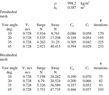
Table 4, Comparison of CFD predictions of hydrodynamic forces, tug with no fin

ρ 998.2 kg/m3

AL 0.387 m2 Tetrahedral

mesh

Yaw angle V, Surge Sway Cq Cl

# iterations

deg. m/s N N

10 0.728 5.916 8.761 0.086 0.058 170

20 0.728 5.535 17.298 0.169 0.054 195

35 0.728 4.262 31.25 0.305 0.042 225

45 0.728 2.921 40.415 0.394 0.029 233

Hexahedral mesh

Yaw angle V, m/s Surge Sway Cq Cl

# iterations

deg. m/s N N

10 0.728 7.198 10.262 0.100 0.070 75

20 0.728 6.79 20.524 0.200 0.066 82

35 0.728 5.326 36.589 0.357 0.052 93

45 0.728 3.751 47.735 0.466 0.037 103

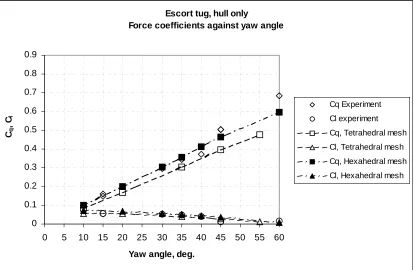
When the force coefficients derived from experimental measurements were compared to the values predicted by CFD, the hexahedral mesh gave the most accurate predictions for the tug with no fin. The average discrepancy between the predicted side force component and the measured value was 6 percent and the maximum discrepancy was 13 per cent. The largest discrepancy between measured and predicted values occurred at 60 degrees of yaw. For the tetrahedral mesh the predicted forces are consistently under predicted by an average of 18 percent when compared to the measured values, with the maximum

For the longitudinal force component, which was much smaller than the side force component at the operating yaw angles, the tetrahedral mesh had an average discrepancy of 1 percent and the hexahedral mesh had an average discrepancy of 4 percent.

Comparisons of the forces were made on the basis of the difference between the measured and predicted value of the force component non-dimensionalized by the total measured force ((Fx2+Fy2)0.5).

Escort tug, hull only

Force coefficients against yaw angle

0 0.1 0.2 0.3 0.4 0.5 0.6 0.7 0.8 0.9

0 5 10 15 20 25 30 35 40 45 50 55 60

Yaw angle, deg. Cq

, C

l

Cq Experiment

Cl experiment

Cq, Tetrahedral mesh

Cl, Tetrahedral mesh

Cq, Hexahedral mesh

Cl, Hexahedral mesh

4.2 Hull & Fin

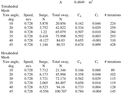
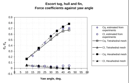
Force components and non-dimensional coefficients derived from the results of the CFD simulations for the combined hull and fin are given for the tetrahedral and hexahedral meshes in Table 5. The results of the simulations are compared with the experiments in Figure 7.

Table 5, Comparison of CFD predictions of hydrodynamic forces, tug with fin

ρ 998.2 kg/m3

A 0.4849 m2

Tetrahedral Mesh

Yaw angle, Speed, Surge, Total sway, Cq Cl # iterations

deg m/s N N

10 0.728 5.878 20.856 0.162 0.046 224

20 0.728 3.752 42.822 0.334 0.029 259

30 0.728 1.22 65.079 0.507 0.010 284

35 0.728 0.418 75.998 0.592 0.003 293

40 0.728 -0.127 84.03 0.655 -0.001 310

45 0.728 1.146 86.53 0.674 0.009 428

Hexahedral Mesh

Yaw angle, Speed, Surge, Total sway, Cq Cl # iterations

deg m/s N N

10 0.728 7.712 21.346 0.166 0.060 89

20 0.728 6.173 45.906 0.358 0.048 102

30 0.728 3.721 72.174 0.562 0.029 115

35 0.728 2.065 84.407 0.658 0.016 119

40 0.728 0.523 94.16 0.733 0.004 128

Escort tug, hull and fin, Force coefficients against yaw angle

-0.1 0 0.1 0.2 0.3 0.4 0.5 0.6 0.7 0.8 0.9

0 5 10 15 20 25 30 35 40 45 50 55 60

Yaw angle, deg. Cl

, C

q

Cq, estimated from experiments Cl, estimated from experiments

Cq, Tetrahedral mesh

Cl, Tetrahedral mesh

Cq, Hexahedral mesh

Cl, Hexahedral mesh

Figure 7, Comparison of CFD predictions for force coefficients with experiment values, hull and fin

The experimental force data for the hull and fin condition was not available, since this was not a condition required for the original project. All of the experiments with a fin included the protective cage. The effect of the cage was estimated from the complete data set by subtracting the force components for the cage (estimated from the hull only

condition and the hull and cage condition) from the hull, fin and cage condition.

meshes are smaller. The hexahedral mesh resulted in predicted forces that were typically within 5 percent of the measured values, and never more than 10 percent different, whereas for the tetrahedral mesh, the typical agreement was within 7 percent and the maximum discrepancy was within 12 per cent. The force coefficients predicted from the hexahedral mesh were all within 5 percent of the experiment data for yaw angles between 30 and 40 degrees and within 10 percent at 45 degrees. The forces predicted by the tetrahedral mesh over this range were typically within 10 percent of the measured forces over the same range of yaw angle, but were consistently under predicted relative to the measured values. The force coefficients predicted by the hexahedral mesh were a good mean fit to the measured values up to 35 degrees of yaw, but above that the forces predicted by CFD are over predicted relative to the measured values.

The predicted normal force (pressure) and tangential force (viscous) components acting on the tug hull (fitted with the fin) from the hexahedral mesh are given in Table 6. These data show that as the yaw angle was increased, the proportion of viscous force to total force decreased. At zero yaw, the viscous force was approximately 25% of the total force, whereas at 10 degrees yaw, this had dropped to 9%, and at 30 degrees yaw it had dropped to 2%. At high yaw angles very little error in the forces at the hull would be expected by ignoring the viscous forces completely. One important element of including the viscosity forces within the fluid is to ensure the formation of vortices within the flow. It is

Table 6, Comparison of pressure and viscous forces acting on tug and fin (hexahedral mesh)

Yaw Pressure Viscous Total Viscous/Total Angle Force Force Force

Degrees N N N

0 6.07 2.06 8.13 0.254 10 22.11 1.93 22.73 0.085 20 46.08 1.71 46.32 0.037 30 72.16 1.45 72.27 0.020 40 94.05 1.14 94.16 0.012

50 102.91 0.88 103.11 0.008

5.5 CFD PREDICTIONS OF FLOW PATTERNS AT 45 DEGREES YAW

X

Y

0 0.5 1 1.5 2

-1 -0.5 0 0.5 1

Downstream plane

Upstream plane

Flow direction (normal to planes)

CFD predictions of flow pattern Planes used for visualization of data matched to PIV experiments

Figure 8, Planes used for comparing predicted flow patterns with PIV measurements

As the grid for the CFD simulations had been created using ship-based coordinates, it was necessary to use the transformations given below, to convert the coordinates and vectors within the CFD simulations to the same flow based coordinate system as the PIV

) Cos Sin

(

) Sin Cos

(

θ θ

θ θ

s s

f

s s

f

y x

y

y x

x

+ −

=

+ =

where;

xf and yf are in the flow based coordinates

xs and ys are in the ship based coordinates

θ is the angle between the flow direction and the ship based coordinates. As the transformation about the vertical axis was purely rotation, the third axis (z in the experiment notation) was unchanged.

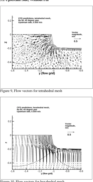
The CFD predictions of flow vectors within the plane and contours of velocity through the plane for the three regions where PIV experiments were carried out are shown below. Figures 9 and 10 show the upstream bilge, Figures 11 and 12 show the downstream bilge, with the fin removed and Figures 13 and 14 show the downstream bilge with the fin present. In each pair of figures, the first figure shows results for the tetrahedral mesh and the second shows results for the hexahedral mesh. Each prediction was made for an undisturbed flow speed of 0.5 m/s.

One notable difference between the results given by the two meshes was that the

5.1 Upstream Side, Without Fin 0.1 0.2 0.3 0. 4 0.4 0.5 0.5 0.5

y (flow grid)

Z

-1.6 -1.4 -1.2 -1 -0.8 -0.6

-0.4 -0.2 0 0.2

0.5

CFD predictions, tetrahedral mesh, No fin, 45 degree yaw,

Upstream side, 0.500 m/s

Vector magnitude, m/s

Figure 9, Flow vectors for tetrahedral mesh

Figure 10, Flow vectors for hexahedral mesh

0.050.1 0.15 0.2 0.25 0.3 0.35 0_.3 5 0.4 0.4 0.45 0 .4 5 0.5 0.5 0.55 0.55

y (flow grid)

Z

-1.6 -1.4 -1.2 -1 -0.8 -0.6

-0.4 -0.2 0 0.2

0.5

CFD predictions, hexahedral mesh, No fin, 45 degree yaw

Upstream side, 0.500 m/s

5.2 Downstream Side, Without Fin

0.05

0.05 0.1

0.15 0.2 0.25 0 .3 0 .35 0.35 0.4 0 .4 0.45 0.45 0.5 0.5

y (flow grid)

Z

-1 -0.8 -0.6 -0.4 -0.2 0 0.2 0.4

-0.6 -0.4 -0.2 0 0.2 0.5

CFD predictions, tetrahedral mesh, No fin, 45 degree yaw

Downstream side, 0.500 m/s

Vector magnitude, m/s

Figure 11, Flow vectors for tetrahedral mesh

0.0 5 0 .1 0.15 0

.2 0.25

0.25 0.3 0.35 0.4 0.4 5 0.45 0.5 0.5 0.55 55

y (flow grid)

Z

-1 -0.8 -0.6 -0.4 -0.2 0 0.2 0.4

-0.6 -0.4 -0.2 0

0.5

CFD predictions, hexahedral mesh, No fin, 45 degree yaw

Downstream side, 0.500 m/s

5.3 Downstream Side, With Fin 0 .1 0.1 0.1 0.2 0.2 0.2 0.3 0.3 0.3 0.4 0.4 0 .5 0.5 0.5

y (flow grid)

Z

-1 -0.8 -0.6 -0.4 -0.2 0 0.2

-0.6 -0.4 -0.2 0 0.2 0.5

CFD predictions, tetrahedral mesh Tug with fin, 45 degree yaw, Downstream side, 0.500 m/s

Vector magnitude, m/s

Figure 13, Flow vectors for tetrahedral mesh

0.05 0 .1 0.1 0.15 0.2 0.2 0.25 0.2₅ 0.3 0.3 0_.3 5 0.35 0.35 0.4 0.4

0.4 0.4

5 0.45 0.5 0.5 0.5 0.55

y (flow grid)

Z

-1 -0.8 -0.6 -0.4 -0.2 0 0.2

-0.6 -0.4 -0.2 0 0.2 0.5

CFD predictions, hexahedral mesh Tug with fin, 45 degree yaw Downstream side, 0.500 m/s

Vector magnitude, m/s

6. QUANTITATIVE COMPARISON OF FLOW PATTERNS PREDICTED BY CFD AGAINST MEASURED PIV DATA

A numerical method was developed for comparing measured flow pattern data with the flow patterns predicted using CFD (Molyneux & Bose, 2007). This data compared the 3-dimensional flow vectors measured in experiments with CFD predictions for the same components over a common plane. This section describes the results of the same analysis applied to the PIV experiments on the escort tug (Molyneux et al., 2007) with the CFD predictions for the same flow conditions described above.

The CFD data was reduced to a plane larger than the area covered by the measurements, but smaller than the complete plane within the CFD simulations. Each velocity

component (Vx, Vy, Vz) was plotted as a contour over the reduced plane. In the PIV experiments two measurement grids were used. One was a fine grid, based on the PIV analysis for a single PIV window. The second grid was a coarser grid of 20mm squares that was used when all the PIV windows were combined and average flow vectors calculated for the complete measurement area. It was the coarse grid that was used for comparison with the CFD results.

cfd t

error V V

V = _exp −

and graphed to show the errors in velocity magnitude and direction.

The following parameters were also used as part of the numerical evaluation of the difference between the experiment values and the CFD predictions:

cfd t z cfd t y cfd t x Vz Vz ErrorV Vy Vy ErrorV Vx Vx ErrorV − = − = − = exp exp exp 2 2 2 3 2 2 2 z y x D z y D ErrorV ErrorV ErrorV Error ErrorV ErrorV Error + + = + =

The results of the numerical analysis for the six flow conditions are shown in Figures 15 to 26, and summarized in Tables 7 to 12.

In each set of results, the first figure shows Verror(magnitude and direction), the second

shows ErrorVx and the table summarizes the results. All results presented are based on the measured or predicted values of the flow speed, and have units of m/s for magnitude and radians for direction. The numerical analysis and visualization of the error between the experimental values and the CFD predictions was carried out using Igor (Wavemetrics Inc., 2005). This is a general-purpose computer program for data analysis and

6.1 Upstream side, without fin, tetrahedral mesh Table 7, Summary of error in CFD prediction

Average Standard

Deviation Minimum Maximum Range

In-plane

Error Vy -0.001 0.068 -0.346 0.134 0.480

Error Vz -0.005 0.023 -0.085 0.162 0.247

Error 2d 0.042 0.059 0.001 0.347 0.345

Through plane

Error Vx -0.066 0.035 -0.238 0.137 0.375

Error 3d 0.086 0.058 0.019 0.347 0.328

-0.35 -0.30 -0.25 -0.20 -0.15 -0.10 z, m

-1.3 -1.2 -1.1 -1.0 -0.9 -0.8 -0.7

y, m 0.30 0.25 0.20 0.15 0.10 0.05 0.00 E rro r 2 d

Figure 15, In-plane error, magnitude and direction

-0.35 -0.30 -0.25 -0.20 -0.15 -0.10 z, m

-1.3 -1.2 -1.1 -1.0 -0.9 -0.8 -0.7

6.2 Upstream side, without fin, hexahedral mesh Table 8, Summary of error in CFD prediction

Average Standard

Deviation Minimum Maximum Range

In-plane

Error Vy 0.001 0.061 -0.282 0.136 0.418

Error Vz 0.001 0.023 -0.064 0.142 0.205

Error 2d 0.038 0.053 0.001 0.282 0.281

Through plane

Error Vx -0.069 0.041 -0.300 0.115 0.415

Error 3d 0.085 0.060 0.018 0.372 0.354

-0.35 -0.30 -0.25 -0.20 -0.15 -0.10 z, m

-1.3 -1.2 -1.1 -1.0 -0.9 -0.8 -0.7

y, m 0.25 0.20 0.15 0.10 0.05 0.00 Er ror 2d

Figure 17, In-plane error, magnitude and direction

-0.35 -0.30 -0.25 -0.20 -0.15 -0.10 z, m

-1.3 -1.2 -1.1 -1.0 -0.9 -0.8 -0.7

y, m -0.3 -0.2 -0.1 0.0 0.1 Er ro r V x

6.3 Downstream side, without fin, tetrahedral mesh Table 9, Summary of error in CFD prediction

Average Standard

Deviation Minimum Maximum Range

In-plane

Error Vy 0.012 0.035 -0.072 0.174 0.246

Error Vz 0.005 0.024 -0.048 0.064 0.112

Error 2d 0.037 0.024 0.002 0.175 0.172

Through plane

Error Vx -0.034 0.050 -0.137 0.187 0.324

Error 3d 0.070 0.027 0.007 0.221 0.215

-0.40 -0.35 -0.30 -0.25 -0.20 -0.15 -0.10 z, m

-0.6 -0.4 -0.2 0.0

y, m 0.16 0.14 0.12 0.10 0.08 0.06 0.04 0.02 Er ro r 2 d

Figure 19, In-plane error, magnitude and direction

-0.40 -0.35 -0.30 -0.25 -0.20 -0.15 -0.10 z, m

-0.6 -0.4 -0.2 0.0

y, m 0.15 0.10 0.05 0.00 -0.05 -0.10 Erro r Vx

6.4 Downstream side, without fin, hexahedral mesh Table 10, Summary of error in CFD prediction

Average Standard

Deviation Minimum Maximum Range

In-plane

Error Vy 0.013 0.040 -0.052 0.200 0.252

Error Vz 0.001 0.022 -0.045 0.063 0.108

Error 2d 0.039 0.028 0.002 0.200 0.198

Through plane

Error Vx -0.040 0.055 -0.110 0.206 0.316

Error 3d 0.078 0.028 0.012 0.219 0.207

-0.40 -0.35 -0.30 -0.25 -0.20 -0.15 -0.10 z, m

-0.6 -0.4 -0.2 0.0

y, m 0.20 0.15 0.10 0.05 Er ro r 2 d

Figure 21, In-plane error, magnitude and direction

-0.40 -0.35 -0.30 -0.25 -0.20 -0.15 -0.10 z, m

-0.6 -0.4 -0.2 0.0

y, m 0.20 0.15 0.10 0.05 0.00 -0.05 -0.10 Er ro r V x

6.5 Down stream side, with fin, tetrahedral mesh Table 11, Summary of error in CFD prediction

Average Standard

Deviation Minimum Maximum Range

In-plane

Error Vy -0.005 0.043 -0.131 0.240 0.371

Error Vz 0.020 0.033 -0.094 0.114 0.208

Error 2d 0.049 0.032 0.002 0.254 0.252

Through plane

Error Vx -0.062 0.068 -0.185 0.307 0.492

Error 3d 0.100 0.044 0.010 0.397 0.388

-0.35 -0.30 -0.25 -0.20 -0.15 -0.10 z, m

-0.6 -0.4 -0.2 0.0 0.2

y, m 0.25 0.20 0.15 0.10 0.05 Er ro r 2 d

Figure 23, In-plane error, magnitude and direction

-0.35 -0.30 -0.25 -0.20 -0.15 -0.10 z, m

-0.6 -0.4 -0.2 0.0 0.2

6.6 Down stream side, with fin, hexahedral mesh Table 12, Summary of error in CFD prediction

Average Standard

Deviation Minimum Maximum Range

In-plane

Error Vy 0.007 0.048 -0.128 0.278 0.406

Error Vz 0.021 0.034 -0.116 0.116 0.232

Error 2d 0.051 0.037 0.000 0.290 0.290

Through plane

Error Vx -0.088 0.052 -0.200 0.278 0.478

Error 3d 0.113 0.039 0.034 0.388 0.354

-0.35 -0.30 -0.25 -0.20 -0.15 -0.10 z, m

-0.6 -0.4 -0.2 0.0 0.2

y, m 0.25 0.20 0.15 0.10 0.05 0.00 Er ro r 2 d

Figure 25, In-plane error, magnitude and direction

-0.35 -0.30 -0.25 -0.20 -0.15 -0.10 z, m

-0.6 -0.4 -0.2 0.0 0.2

y, m 0.2 0.1 0.0 -0.1 -0.2 Er ro r V x

7. DISCUSSION OF EXPERIMENTAL RESULTS

7.1 Through Plane Velocity Components

Table 13 shows a summary of the non-dimensional errors in the through plane velocity components for each of the locations around the tug. In this table, the non-dimensional parameter Erroru(which is the error in the through-plane velocitycomponent) was calculated from Tables 7 to 12 by non-dimensionalizing the values of ErrorVx with the free stream flow speed.

Table 13, Non-dimensional values of Erroru

Flow region Tetrahedral

mesh

Hexahedral mesh Upstream, no fin -0.133 -0.138 Down stream, no fin -0.068 -0.080 Downstream, with fin -0.124 -0.175

7.2 In-plane Velocity Components

Three numerical values were picked to compare the PIV experiments with the tetrahedral and hexahedral meshes. These were the mean value and standard deviation of Error2D and the fraction of the data where the error between the CFD predictions and the experiments (for the in-plane flow components) were within 10% of the free stream speed. The values were non-dimensionalized based on the free stream speed of 0.5 m/s. The results are given in Tables 14 to 16.

Table 14, Non-dimensional mean, Error2D

Flow region Tetrahedral

mesh

Hexahedral mesh Upstream, no fin 0.083 0.076 Down stream, no fin 0.074 0.078 Downstream, with fin 0.097 0.101

Table 15, Non-dimensional standard deviation, Error2D

Flow region Tetrahedral

mesh

Hexahedral mesh Upstream, no fin 0.117 0.107 Down stream, no fin 0.049 0.055 Downstream, with fin 0.064 0.074

Table 16, Fraction of data set where Error2D was within 10% of free stream speed

Flow region Tetrahedral

mesh

Hexahedral mesh Upstream, no fin 0.827 0.840 Down stream, no fin 0.820 0.785 Downstream, with fin 0.623 0.598

experiments. The hexahedral mesh had a small advantage on the upstream side of the tug model, but on the downstream side, the tetrahedral mesh had a slight advantage. In general, the best predictions were for the upstream side of the tug and the worst

predictions were for the downstream side of the tug, with the fin. This was to be expected since the downstream side of the flow was much more unsteady (Molyneux et al., 2007b).

For the flow on the upstream side of the hull (Figures 17 and 19), both meshes gave similar errors, with the worst predictions of flow vectors close to the hull and the accuracy of the predictions improving as the distance from the hull increased. PIV measurements close to the hull will likely be the most difficult to obtain accurately, because the hull, even when painted black, reflects the light and a bright band is seen in the pictures of the particles where the laser beam cuts the hull. Even though the analysis software includes a filter to reduce this effect, the experiment results obtained in this region may be subject to error.

the region where the strongest flow velocities occurred. These high velocities were the result of the vortex caused by the flow separation off the corner of the bilge. Again the hexahedral gave smaller errors in this region but the difference was not significant relative to the tetrahedral mesh.

When the fin was present (Figures 23 and 25) and the very large vortex was generated, the worst comparison between the experiment data and the CFD predictions occurred close to the hull on the downstream side between the bottom of the hull and the waterline, and under the hull. Both meshes showed relatively small errors in the flow around the vortex, but the hexahedral mesh gave relatively poor prediction of the flow patterns close to the waterline, compared with the tetrahedral mesh.

Based on the numerical analysis, both meshes gave similar predictions of the flow patterns around the hull of an escort tug with a yaw angle of 45 degrees, and neither approach had a significant advantage in any of the conditions investigated.

Table 17, Comparison of errors in velocity magnitude for in-plane vectors, Series 60 and escort tug, tetrahedral mesh

Parameter Series 60, CB=0.6

Yaw angle 35 degrees,

Midship section

Escort tug, no fin Yaw angle 45 degrees,

Midship section

Escort tug, with fin Yaw angle 45 degrees,

Midship section

Errorv 0.091 0.024 -0.01

Errorw 0.013 0.010 0.040

Error2D 0.241 0.070 0.098

Table 18, Comparison of errors in velocity magnitude for in-plane vectors, Series 60 and escort tug, hexahedral mesh

Parameter Series 60, CB=0.6

Yaw angle 35 degrees,

Midship section

Escort tug, no fin Yaw angle 45 degrees,

Midship section

Escort tug, with fin Yaw angle 45 degrees,

Midship section

Errorv 0.053 0.027 0.014

Errorw 0.049 0.003 0.042

Error2D 0.164 0.078 0.102

These differences may be due to the significant differences in the hull shapes between the escort tug and the Series 60 hull. The escort tug was proportionally much wider

8. RECOMMENDATIONS FOR FURTHER STUDY

There are some improvements that could be made to the CFD mesh that might improve the level of prediction of the forces and flow patterns. The first major refinement would be to include the free surface waves generated by the hull. This was ignored from the current meshes on the basis that the effect of the free surface on the forces measured in the model experiments was seen to be small. The free surface of the water will distort and may affect the flow patterns close to the surface. This effect will become more noticeable as yaw angles and flow speeds increase.

Another refinement would be to make the mesh elements smaller in key areas of the flow. The most likely areas for refinement are where vortices are generated in the flow. The most noticeable vortices observed in the PIV experiments were around the downstream bilge for the hull without the fin, and the large vortex generated by the fin when it was fitted. A refined mesh could be generated and the results compared with the single measurement window PIV data (Molyneux et al. 2007), instead of the coarser data spacing that was used for the complete data set.

9. CONCLUSIONS

were used. One type was a tetrahedral mesh, consisting of elements with four, three sided faces. The other type was a hexahedral mesh, consisting of elements made of six four sided faces. The most accurate force predictions were obtained using the mesh made entirely of hexahedral elements. This mesh gave force predictions that on average were within 5-6 % of measured values for the same flow conditions, and never exceeded 10%. The number of elements for the hexahedral mesh was less than one half of the number in the tetrahedral mesh, which resulted in a faster solution time.

The flow patterns around the hull predicted by both meshes at 45 degrees yaw were compared to PIV measurements taken at two planes around the hull. A subjective comparison of the results indicated that the hexahedral mesh gave slightly better predictions of the flow patterns, especially for the flow conditions across the bottom of the hull. A numerical analysis comparing the two meshes over the complete measurement region indicated that the differences were very localized and numerically very small. The average difference between the measured and predicted in-plane flow velocity vector magnitudes was between 8 and 10 per cent.

predictions for different meshes, since this hull was wide and shallow with a high degree of curvature, whereas the Series 60 was relatively narrow with very sharp waterlines in the bow and stern. This narrow entrance angle for the Series 60 hull creates a vortex, which is generated from the keel at the bow and moves towards the downstream side of the hull. For the escort tug, the fin is the only thing creating a large vortex, and the flow remains attached to the hull, even on the down stream side.

10. ACKNOWLEDGEMENTS

The work described in this paper would not have been possible without the help and support of many people, which is gratefully acknowledged:

Mr. Robert Allan, President of Robert Allan Ltd., Vancouver, British Columbia, for permission to use the model of the escort tug in the PIV experiments and for the use of the experimental data on the force components to compare with the CFD simulations. His enthusiasm for the subject of tug design and encouragement for me to carry out this work is also very much appreciated.

Ms. Jie Xu, research laboratory coordinator in the Department of Ocean and Naval Architectural Engineering, for her leadership, continuous dedication and attention to detail that was necessary for making successful PIV experiments.

Mr. Jim Gosse, Laboratory Technician in the Fluids Laboratory at Memorial University is for all his help during the set-up and carrying out the preliminary PIV experiments in the OERC Towing Tank at MUN.

The staff at IOT for preparing the model for testing and assisting with the many tasks required during experiments at IOT, together with their financial support.

The management of IOT is thanked for their financial support.

11. REFERENCES

Allan R. G. & Molyneux, W. D. 2004 ‘Escort Tug Design Alternatives and a Comparison of Their Hydrodynamic Performance’, Paper A11, Maritime Technology Conference and Expo, S.N.A.M.E. Washington, D. C. September 30th to October 1st.

Fluent Inc. 2005(a) ‘Fluent 6.2 User’s Guide’, available on-line, July 2005.

http://www.fluentusers.com/fluent/doc/ori/html/ug/main_pre.htm

Fluent Inc. 2005(b) ‘Gambit 2.2 User’s Guide’, available on-line, June 2005

http://www.fluentusers.com/gambit/doc/doc_f.htm

Hutchison, B., Gray, D. and Jagannathan S., 1993 ‘New Insights into Voith Schneider Tractor Tug Capability’, Marine Technology, Vol. 30, No. 4, pp. 233-242.

Molyneux, W. D. and Bose, N., 2007 ‘A quantitative Method to Compare Results from Different CFD simulations and Experimental Data’, Submitted to Journal of Ship Research, SNAME.

Molyneux, W. D., Xu, J. and Bose, N. 2007a), ‘Commissioning a Stereoscopic Particle Image Velocimetry System for Application in a Towing Tank’, Proceedings, 28th

American Towing Tank Conference, University of Michigan, Ann Arbor, MI, August 9-10th, 2007.

Molyneux, W. D., Xu, J. and Bose, N. 2007b) ‘Measurements of flow Around an Escort Tug Model With a Yaw Angle’, submitted to Marine Technology, SNAME

Rhee, S. H. 2005, Lead Consulting Engineer, Fluent Inc., Private correspondence by email, 11 July.

Turnock, S. 2006, Senior Lecturer in Ship Science, University of Southampton, Private correspondence by email, 7 April.

Van den Braembussche, R. A. (editor) 2001 ‘Measurement Techniques in Fluid Dynamics’, Von Karman Institute for Fluid Dynamics, 2nd Revised Edition.